Jun 26, 2006 - b - Some states use API data until 2002 rather than DeGolyer and Mac-. Naughton data ...... Shell Development Company. [20] Marion King ...
Testing Hubbert Adam R. Brandt∗
Energy and Resources Group University of California, Berkeley June 26th, 2006
Abstract The Hubbert theory of oil depletion, which states that oil production in large regions follows a bell-shaped curve over time, has been cited as a method to predict the future of global oil production. However, the assumptions of the Hubbert method have never been rigourously tested with a large dataset. In this paper, the Hubbert theory of depletion is tested against five alternative models, using a set of 139 oil production curves. These curves are sub-national (United States state-level, United States regional-level), national, and multinational (subcontinental and continental) in scale. Best-fitting curves are generated for each region using the six models, and the quality of fit is compared across models. We also test two assertions that have been made with respect to oil depletion: that production over time in a region tends to be symmetric, and that production is more bell-shaped in larger regions than in smaller regions. ∗
I would like to gratefully acknowledge the assistance of Anand Patil, Alex Farrell, and Jim Kirchner in the preparation and revision of this paper.
1
1
Introduction and context
Since nearly the beginning of commercial exploitation of oil, there has been great interest in two related questions: how much oil exists in the world, and when will humanity run out of oil? This very old discussion has recently resurfaced, as general interest in oil depletion has increased along with increasing oil prices. Recent projections of global oil production have been made using the Hubbert theory of oil depletion, and these projections have been rejected by those who doubt the effectiveness of the method. Importantly, however, the Hubbert theory has never been rigourously tested with any large dataset, and many Hubbert-type predictions are based on proprietary datasets, all but precluding the process of peer review. This paper aims to test some aspects of the Hubbert theory against other plausible theories of how oil production varies over time.
The Hubbert theory of oil depletion The Hubbert theory of oil depletion was first presented in 1956 by M. King Hubbert, a senior research geologist with Shell Oil [19]. As presented in his 1956 paper, he made projections of future United States oil production based on two estimates of the total amount of oil that would be produced in the United States. He did not provide a functional form for his prediction in this early paper, but instead fit past production to a bell-shaped curve in which the area under the curve was equal to his predictions of the amount of total oil production. Using this method, he arrived at two predicted dates for peak production, one in the mid-1960s, the other around 1970. By 1959, he had added other elements to his analysis [20]. First, he specified a functional form, the logistic curve, stating that cumulative production over time would follow a logistic curve, and thus that yearly production
2
would follow the first derivative of the logistic curve, which is bell-shaped. He also analyzed patterns of discovery and production. He plotted cumulated discoveries alongside cumulated production and noted that the curves were similar in shape but shifted in time [19]. With this paper, most of the major elements of modern Hubbert analysis were developed. United States oil production peaked in the early 1970s, and with this vindication the Hubbert theory became an important tool for those concerned about depletion of natural resources [13]. This success caused Hubbert and others to project future global oil production. The recent explosion of interest in the Hubbert theory started in the 1990s with Colin Campbell’s efforts to use it to predict global oil production [9]. As currently practiced, Hubbert modeling is really a constellation of techniques, many of which were developed by Hubbert himself in his early papers. The methods used vary widely by analyst, but the core techniques of modern Hubbert analysis are as follows: Analysis of past discoveries - regional discovery data are plotted, and sometimes adjusted for reserve growth, and a best-fitting curve (typically Gaussian) is matched to discoveries. Estimation of future oil discoveries - future amounts of oil remaining to be found are extrapolated in a number of ways, including estimating an asymptote for discovery growth when plotting cumulative discoveries by cumulative wells drilled [9]; by using a newer technique sometimes called “Hubbert linearization” to project ultimate recovery [13]; or by using a statistical relationship such as the parabolic fractal law to attempt to infer the size distribution of remaining fields using the distribution of already-discovered field sizes [22]. Projection of future production - using discovery data in conjunction 3
with estimated future production, a curve (again, typically Gaussian) is fit to historical production data such that the area under the curve equals the sum of discovered and yet-to-find oil. Hubbert modeling, as typically practiced, includes a number of assumptions, including: that production follows a bell-shaped curve; that production is symmetric over time (i.e. the decline in production will mirror the increase in production, and the year of maximum production, or peak year, occurs when the resource is half depleted); that production will follow discovery in functional form and with a constant time lag; and, lastly, that production increases and decreases in a single “up-down” cycle without multiple peaks.
Alternative models of oil depletion A number of models of oil depletion have been used over time to forecast future oil production. The most simple of these models, and often not thought of as a “model” at all, is the reserve to production ratio (R/P), or simply the quantity of current reserves divided by current production. Criticisms of this methodology are too numerous to cite, but the general problem with this analysis is that neither reserves nor production are constant over time, making it nearly valueless as a forecasting technique. Modified versions of the Hubbert methodology have been developed. These include a model by Hallock et al. which uses a modified version of the bell-shaped curve, with a peak at 60% of ultimate production instead of the typical 50% [17]. This method implies an asymmetric shape to production and a steeper rate of decline than increase. Another simple model is a linear oil depletion model, where production increases linearly and then declines linearly as well, but such a model has never received much attention, likely due to its poor fit to smooth-topped 4
production curves. However, Hirsch [18] notes that United States production in the period 1945-2000 fits a linear production profile better than a bellshaped curve. Exponential models are another possible simple model. Hubbert used an exponential fit in the 1956 paper where he first presents his method, plotting United States coal and oil production on a semi-logarithmic scale, noting the straight line over much of history. A straight line on such axes indicates exponential growth [19]. Also, Wood et al., in a more modern analysis, assumed a 2% exponential growth for world oil production, followed by a decline “at an R/P ratio of 10” [31]. This decline at a constant R/P of 10 is equivalent to exponential decline of 10% per year. Hirsch studied peaking rates of a small number of production regions, including the United States, Texas, the United Kingdom, and Norway, and noted that production peaks have tended to be steeper and sharper than predicted by the Hubbert theory [18]. Some bottom-up modeling efforts, using models that simulate finding and extracting resources over time, suggest that production would be roughly bell-shaped, but not necessarily symmetric [7, 30]. Bardi critiques the assumption of symmetrical production over time, stating that there is “no magic in the ‘midpoint’ of the production of a mineral resource” and that production can exhibit a decline rate greater than the rate of increase [7].
Problems with current depletion analysis There are significant difficulties with current methods of predicting future oil production. Two classes of problems emerge: those resulting from poor data, and those resulting from uncertain methodologies. The first class of problems stems from poor access to data on oil production and reserves. Even if it were agreed that the Hubbert methodology 5
was effective in projecting future production, data unavailability would still hinder analysis. This is for two reasons. First, there is still uncertainty with respect to remaining volumes of oil to be found. This uncertainty is likely decreasing over time as exploration continues. Andrews and Udall and Ahlbrandt have collected projections of estimated ultimate recovery of oil (EUR), plots of which suggest that we are perhaps asymptotically approaching stable estimates of total conventional oil recoverable [1, 2]. Second, there is no access to data from many countries, including the producers that are most likely to influence the date of peak production, such as OPEC. This lack of data manifests itself repeatedly and in multiple guises in Hubbert-type analysis. Most analysts using the Hubbert methodology have used proprietary datasets which are not accessible except at high cost [9, 10, 11]. Most publicly available datasets only contain data back to the 1970s or 1960s [8, 16]. This discrepancy between the data used by Hubbert theorists and available data makes checking their work impossible and invites skepticism of their results [24]. Another manifestation of poor data availability is that most studies rely on a small number of cases, such that the United States is plotted many times, but other regions are not. Campbell [12] plots dozens of curves, but Lynch states that “in Campbell (2003)...only 8 of 51 non-OPEC countries” appear to follow a bell-shaped curve [24]. Certainly Campbell would disagree with this assessment, but it is difficult to determine who is correct in such a situation without access to the underlying data. Additionally Campbell’s plots often do not distinguish between historical data and projections and he does not discuss the quality of the model fit to data [9, 12]. This makes it difficult to estimate even qualitatively the goodness of fit of his figures. The second set of problems for predicting the future of oil production is due to uncertainty about methodologies. Perhaps the most fundamental
6
points of confusion are that many types of predictions are made, definitions of what is being predicted are often unclear, and there is disagreement about what quantities are important to predict. Campbell is quite clear in his definitions of what is being predicted [10], focusing on “conventional” oil, and separating these production data from deep offshore, heavy oil, etc. Others, more economically oriented, pay less mind to the distinction between these resources [29] and emphasize the substitutability of resources [21]. These groups argue as if they are producing comparable estimates, when often they are not. In essence, these groups disagree about what the “important” quantity is: Hubbert modelers are interested in production and depletion of conventional oil, and often dismiss alternatives such as low-quality petroleum resources, while economic observers are interested primarily in the transition to substitutes for conventional oil, and they find the question of the depletion of a specifically defined resource uninteresting or unimportant. Not surprisingly, it is difficult to find agreement between the parties when the questions they ask are different. Most Hubbert analyses are based on the Gaussian curve, although some are based on the very similar logistic curve [13]. This leads to another methodological difficulty: the justification for the use of the Gaussian curve in predicting future production. Laherrere [23] states that the Hubbert theory works best with large numbers of disaggregated producers, based on the central limit theorem (CLT), which is the justification for the use of the Gaussian curve in statistical applications. Laherrere states that that in the lower-48 states of the United States “there are over 20,000 producers acting in random,” leading to a Gaussian curve. As has been argued previously, there is little theoretical basis for the assumption of a Gaussian production curve based on the CLT [6]. There are two problems with citing the CLT in this way. First, the CLT traditionally
7
applies to points of data where the independent variable is the measured value of a characteristic and the dependent variable is the number of measurements of that value that are recorded (such as the number of children of height 1 m). Petroleum production curves measure production per unit time (e.g. barrels or m3 per year), not the traditional dimensions for normally distributed phenomena. More importantly, the CLT applies only to distributions that are summed and independent of one another. While the first criteria is met, the second criterion is not met. Production at a given oil field is determined at least in part by the decisions of the producers. These producers, across regions, nations, and even at a global level, respond to common stimuli. At a regional level, common stimuli include local transport costs, availability of nearby markets, and regulatory pressures (such as state or provincial environmental mandates), while national politics can force production up or down, particularly in nations with central control over production (e.g. OPEC). And, of course, at the global scale, both long and short-term trends influence producers simultaneously across the globe. Thus, there is no theoretical reason to expect the CLT to hold. This does not mean that production could not, in reality, follow a Gaussian shaped production function, but that there is no a priori reason to suspect that that it will. Given these difficulties with current methodologies, we seek to test certain assumptions made during Hubbert analysis.
2
Methods of analysis
In this paper we perform three tests of the Hubbert theory. We first seek to test two assumptions of the Hubbert model. We ask if the Gaussian Hubbert model fits historical production data better than five other simple
8
models. We then ask if regional oil production curves have been historically symmetric. Lastly, we test a commonly made assertion about oil depletion: that the Hubbert model fits larger regions better than smaller regions, due to a “smoothing” behavior resulting from summing smaller production curves. We emphasize that we do not test the predictive ability of the Hubbert model, but simply examine the validity of these assumptions using historical data.
Datasets used We attempted to collect the largest possible number of production curves for analysis. Data were collected or compiled at 4 scales: United States statelevel, United States regional-level (created by summing state-level data), national-level, and multi-national-level (such as continental or sub-continental). The sources and years included in these data are shown in Table 1. The regions studied are listed in Table 2. These data series are formed by joining two or more separate series, becuase early production data were only available in earlier reference volumes. In the vast majority of cases the transition between datasets was smooth (i.e. values were equal in both datasets for overlapping years near the transition). This is even the case between DeGolyer and MacNaughton data and API data, suggesting that these sources obtained their data from similar sources. Data were purposely collected at all production scales. Data for smaller regions were summed into larger aggregate regions to acknowledge that production statistics are collected for regions that are arbitrarily defined with respect to geology. Some states in the United States are the size of nations, while some nations are nearly the size of continents (e.g. Former Soviet Union). This aggregation of smaller regions into larger regions creates a smoother spectrum of regional sizes. The definitions of the regions 9
Table 1: Datasets used in analysis Dataset namea Source Years API [3] 1859-1946 API [5] 1947-1989 DeGolyer and [14] 1990-2004b MacNaughton US Regional Level API [3] 1859-1946 API [5] 1947-1989 DeGolyer and [14] 1990-2004 MacNaugton National Level API [4] 1859-1964 DeGolyer and [14] 1965-2004 MacNaughton World Regional Level API [4] 1859-1964 DeGolyer and [14] 1965-2004 MacNaughton a - Data for some regions, specifically Sudan, Morocco, and Equatorial Guinea, were collected from the EIA’s International Energy Annual 2003 [15] because these regions were not included in [14]. b - Some states use API data until 2002 rather than DeGolyer and MacNaughton data from 1990 to 2004. Included in these states are Arizona, Louisiana, Nevada, Texas, and Washington. These regions suffered from inconsistent regional definitions that made them incomparable to the earlier data series. Regional level US State Level
are shown in Appendix A.
Methodology to determine best fitting model in each region The first Hubbert theory assumption we test is whether a bell-shaped production curve fits past production data more accurately than other simple models. To this end, we test the Hubbert model against five other models. These six models are of two types: symmetric three-parameter models (Hubbert, linear, exponential) and asymmetric four-parameter models (asymmetric Hubbert, asymmetric linear and asymmetric exponential). Two tests are conducted: first, the three symmetric models are compared, and all then six models are compared. These tests will be referred to as the three-model comparison and the six-model comparison. 10
Table 2: Regions analyzeda United States state-level Alabama Alaska Arizona Arkansas California Colorado Florida Illinois Indiana Kansas Kentucky Louisiana Michigan Mississippi Missouri Montana Nebraska Nevada New Mexico New York North Dakota Ohio Oklahoma Pennsylvania South Dakota Tennessee Texas Utah Virginia Washington West Virginia Wyoming
United States regions and divisions New England Middle Atlantic East North Central West North Central South Atlantic East South Central West South Central Mountain Pacific Northeast Midwest South West West of Miss. River East of Miss. River Lower-48
Nations
Nations cont.
Sub-continents and continents Middle Africa Northern Africa Western Africa Caribbean Central America South America Northern America Central Asia Eastern Asia Southern Asia South-Eastern Asia Western Asia Eastern Europe Northern Europe Southern Europe Western Europe Australia and NZc Melanesia Africa Americas Asia Europe Oceania World
Albania Mexico Algeria Morocco Angola Netherlands Argentina New Guinea Australia New Zealand Austria Nigeria Bahrain Norway Bolivia Oman Brazil Pakistan Brunei/Malaysia Peru Bulgaria Philippines Burma Poland Cameroon Qatar Canada Republic of Congob Chile Rumania China Saudi Arabia Columbia Spain Czechoslovakia Sudan Denmark Syria Ecuador Thailand Egypt Trinidad Equatorial Guinea Tunisia FSUd Turkey France UAEe Gabon United Kingdom Germany United States Greece Venezuela Hungary Yemen India Yugoslaviaf Indonesia Zaireg Iran Iraq Italy Japan Kuwait Libya a - The regional definitions for the grouping of US state-level and world regional data are shown in Appendix A, which is available at http : \\abrandt.berkeley.edu\hubbert b - The Republic of the Congo is listed simply as “Congo” in the datasets and any graphics from this research. c - Australia and New Zealand d - Former Soviet Union. Data for the FSU are as follows: From 1859 to 1930 are API data for “Russia”. From 1931 to 2004 are DeGolyer MacNaughton data for “Former Soviet Union.” e - United Arab Emirates f - Yugoslavia in recent DeGolyer MacNaughton datasets is listed as “Former Yugoslavia.” g - The Democratic Republic of the Congo, sometimes known as Congo-Kinshasa, is referred to in the dataset used in this research as “Zaire” because data collected from early sources use its older name of Zaire.
11
Table 3: Six studied models and their featuresa Model Number Parameters fit by software of parameters Hubbert 3 Maximum production, year of maximum production, standard deviation of production curve Linear 3 Year of first production, year of maximum production, slope of increase and decrease Exponential 3 Year of first production, year of maximum production, rate of increase and decrease Asymmetrical 4 Maximum production, year of maximum producHubbert tion, standard deviation of increasing side of production curve, standard deviation of decreasing side of production curve Asymmetrical 4 Year of first production, year of maximum prolinear duction, slope of increase, slope of decrease Asymmetrical 4 Year of first production, year of maximum proexponential duction, rate of increase, and rate of decrease a - The mathematical formulation of each of these models is given in Appendix B. These models were tested using the non-linear modeling function of the JMP statistical software package. For each of these models, there are a number of parameters that can vary, such as peak year, rates of change, and year of first production. These parameters are adjusted by the statistical software so as to minimize the sum of squared errors (SSE). The values of the parameters that minimize the SSE represent the best fit for that model. The models are listed in Table 3, along with the parameters fit by the software in each of the models. The mathematical formulation of the models is shown in Appendix B. Schematics of each of the models are illustrated in Figure 1, while regions that are fit well by each of the six models are shown in Figure 2. Comparing models After the non-linear fitting algorithm determines the best values of the model parameters, we can compare the quality of the fit across models to determine 12
1000
800
800
800
600
Production
1200
1000
Production
1200
1000
Production
1200
600
600
400
400
400
200
200
200
0 1900
1925
1950
1975
0 1900
2000
(a) Gaussian Hubbert production curve
1925
1950
1975
0 1900
2000
(b) linear production curve
800
800 Production
1000
800 Production
1200
1000
Production
1200
1000
600
400
400
200
200
200
0 1925
1950
1975
2000
(d) asymmetric Hubbert production curve
1900
1925
1950
1975
2000
(e) asymmetric linear production curve
1975
2000
600
400
0 1900
1950
(c) exponential production curve
1200
600
1925
0 1900
1925
1950
1975
2000
(f) asymmetric exponential production curve
Figure 1: Schematic illustrations of the six tested models
which of the models studied is most appropriate for each region. There is no single method to determine which model fits best, and it must be emphasized that it is impossible to determine, statistically or otherwise, which model is truly “correct,” or even to definitively say which model fits best [25]. Given these uncertainties, the methodology used to assign a most appropriate model to each region is described below. After all models are fit to all regions, we next discard regions where the fitting process is fundamentally flawed. One flaw is insufficient data to make a meaningful fit (only New England and Washington state, with 0 and 4 years of production, respectively). Regions are also discarded because they do not conform to one of the basic assumptions of the models tested. The Hubbert model, as well as all other models tested, assume that production rises and falls in a single cycle. They also implicitly assume that the pro13
(a) Hubbert fit to Wyoming production data
(b) Linear fit to Southern European production data
(c) Exponential fit to Caribbean production data
(d) Asymmetric Hubbert fit to Alabama production data
(e) Asymmetric linear fit to Cameroon production data
(f) Asymmetric exponential fit to Albanian production data
Figure 2: Fit of models to six regions which the models fit well. In each graph, production data are in kbbl/y.
duction is in some sense predictable (i.e. not stochastic). Some regions do not conform to these expectations and have multiple peaks that are separated by multi-decade time periods, such as in Figure 3(a), while others have production that is so chaotic that no one of the tested models can be seen, in practical terms, as more accurate than another, as in Figure 3(b). It must be emphasized that these regions are not disqualified because the software cannot fit the models to the data, but that, in practical terms, the mathematical “good fit” produced to such data means little. In total, 16 of the 139 regions were disqualified and labeled nonconforming because of these reasons. These disqualified regions were not analyzed in either the three-model comparison or the six-model comparison. The disqualified regions include: Arkansas, Illinois, Indiana, New York, Ohio, Pennsylvania, Virginia, Washington, New England, Middle Atlantic, North-
14
(a) Ohio production, a region with multiple temporally dispersed peaks
(b) Iraq, a region with fundamentally chaotic production
Figure 3: These production curves, among others, were eliminated from the comparison process because of fundamental problems in determining a best fit.
east, Burma, Iraq, France, Philippines, and Poland. In addition, 6 other regions were classified as borderline-nonconforming, but were still analyzed: Central Asia, FSU, Saudi Arabia, Southern Asia, Venezuela, and Western Asia. After these models are disqualified, we perform the three-model and sixmodel comparisons. Three-model comparison (comparing only symmetric models) For the three-model comparison, we first analyze the total amount of error over all points between the best-fitting curve and the data. The most basic numerical measures of overall fit are the sum of squared errors (SSE) and the root mean square error (RMSE). Unfortunately, these measures do not properly account for the number of parameters in a model. Any model can be made more complex by adding parameters, such as the differing rates of increase and decrease used in the asymmetric models in this analysis. More complex models nearly always fit better when measured by SSE because they are more flexible. However, the better fit of the more complex model may or may not be justified by the amount of complexity created by additional 15
parameters. A number of approaches exist to deal with this problem [25]. We use Akaike’s Information Criterion (AIC) because it allows us to compare models that are not mathematically “nested” (models are nested when one model can be written as a simplified version of the other). AIC allows us to compare models of different complexity while accounting for the advantage that a more complex model has in fitting [25]. The AIC score (actually the corrected AIC score, the AICc score1 ) is given as follows: µ
SSE AICc = N · ln N
+ 2K +
2K(K + 1) N −K −1
(1)
Where: AICc = corrected AIC score, N = number of data points in data series, SSE = sum of squared errors, and K = number of model parameters.
The model with the smallest AICc score is the most likely to be the best-fitting model [25]. We can also calculate how much more one model is likely to be correct compared to another by using the difference in AICc scores. Because AIC is based on information theory, not statistics, we cannot correctly “reject” or “accept” a model as statistically significant. We can however, determine the probability that one model is correct when compared to another [25], given by the equation:
Probability =
e−0.5·∆AIC 1 + e−0.5·∆AIC
(2)
Where: 1
The AICc is corrected to account for errors that can occur with AIC when the number of datapoints is small.
16
(a) Hubbert fit
(b) Linear fit
Figure 4: Fit of two models to production data from Hungary. See residuals in Figure 5. ∆AIC = (AICc of best-fitting model) - (AICc of second best-fitting model). In the results below, we considered a best-fitting model to have “strong evidence” of being the correct model if it has >99% chance of being the correct model when compared, using Equation 2, to the second best-fitting model. Even a corrected numerical measure of fit, such as AICc cannot tell us which model fits best. We also must visually inspect the models for goodness of fit. This is because there are regions where the total numerical error is minimized by a given model, but there is systematic divergence between the model and the data, or the best-fitting model is nonsensical (e.g. negative decline rates resulting in ever-increasing post-peak production). Thus, in addition to numerical analysis with AICc , all model fits were visually inspected for goodness of fit. If the best fitting model in each region does not have strong evidence, as defined above, the residuals of the models were compared. The residual for each data point is the difference between what the best-fitting model predicts and the actual value. When comparing models, a better model fit results in residuals that are (a) smaller in mag-
17
(a) Residuals from the Hubbert fit
(b) Residuals from linear fit
Figure 5: Residuals from fitting two models to Hungarian production. nitude, (b) more evenly spread around zero (normally distributed), and (c) have fewer trends (i.e. fewer long runs of consecutive points above or below zero) [25]. For some regions it was difficult or impossible to judge if one model or another fit better. In these cases, the AICc was sufficiently close between two models so as to not provide strong evidence (probability < 99%), and inspection of the residuals provided no obvious choice. For this paper, the best-fitting model in these cases is left undetermined. As an example, see Figures 4(a) and 4(b), which show the Hubbert and linear fit for Hungary, a region that was among the most difficult to determine the best-fitting model. Also see Figures 5(a) and 5(b), which show the residuals to these fits. AIC favors the Hubbert model, but not strongly (80% probability). In favor of the linear model, we see smaller maximum error and less consistent error, as well as a somewhat better fit at peak for the linear model. Arguments in favor of the Hubbert model include the better overall numerical fit (lower AICc score), and that the curve does have some “rounded” characteristics. In this paper we chose the Hubbert model, but arguments could be made for classifying this region as undetermined or linear.
18
Six-model comparison (symmetric and asymmetric models) We compare all six models using a similar method to that used for the comparison for the three symmetric models. Recall that the AICc accounts for the increased complexity of the asymmetric models and compares this to the amount of reduction in error produced. In addition to the 16 regions that are disqualified as nonconforming from both the three-model and six-model comparisons, additional regions are disqualified from the six-model comparison. We disqualify all regions that lack sufficient data so as to cause any of the asymmetric models to have difficulty in fitting the curve. Because the asymmetric models include the rate of decline of the production curve as a parameter, the software cannot determine values for these parameters without sufficient data beyond a peak in production. In total, 49 regions are not included in the six-model comparison for this reason. Consequently, the six-model comparison is performed with 74 regions (36 state and multi-state, 38 nations and groups of nations).
Methodology to test the symmetry of regional oil production Another important assumption of Hubbert modeling that has not been rigourously tested is that oil production is assumed to be symmetric over time. In order to test this assumption, we compare best-fitting incline and decline rates. Only the 74 regions that were included in the six-model comparison were used in this test. It is likely that at least a few of these slopes, fit here as post-peak downslopes, will in the future be realized as temporary declines in production and not as a final decline. However, the choice of regions included is also somewhat conservative, such that regions that are thought to have recently peaked, such as the United Kingdom and Norway, are not included because they do not have enough post-peak data for 19
adequate fit. We conduct two simple tests to gain insight into the best-fitting rates of increase and decrease. First, we examine the distribution of best-fitting rates of increase and decrease in the asymmetric exponential model, rinc and rdec . We then study the distribution of a quantity we will call the rate difference, which is the difference between the best-fitting rates of increase and decrease for each region. Thus, the measure of rate difference (∆r) is defined as:
∆rexponential = rinc − rdec
(3)
Methodology to test the quality of the Hubbert fit across regions of different sizes Some Hubbert theorists have suggested that larger regions may fit the Hubbert model more closely, due to a “smoothing” behavior, whereby aberrations in production from differing regions will cancel each other out when summed. In order to test this, the quality of fit was compared across regions of different “size.” We test using both the area of regions (area in km2 ), and total production to date (in cumulative bbl). In order to compare fit across different size regions, a “scale-invariant” measure of fit is required. That is, one needs a measure of fit that is comparable across regions as diverse as Arizona (peak production 3,370 kbbl/y) and Asia (peak production 14,419,387 kbbl/y). SSE and RMSE are poor measures because the absolute amount of error increases as the amount of production increases, even if the percentage error is the same. For this reason, a normalized RMSE was used. In this case, RMSE for each region was divided by the mean production from that region. This normalizes the
20
RMSE by the scale of production and makes regions comparable2 .
3
Results
Best-fitting model results One important general result is that 16 regions were disqualified from both the three-model and six-model comparisons as non-conforming, and 6 more were classified as borderline non-conforming. The disqualified regions are not a significant portion of global production (about 3% of 2004 production), but when we add the borderline non-conforming regions (most importantly Venezuela, Saudi Arabia and FSU), these regions represent 36% of global production. That fully a third of global production is not well characterized by models with a single up-down cycle is a significant result suggesting that these models are not useful in a number of important cases. Specific results about the applicability of each of the models are described below. Three-model comparison: best fit between symmetric models In our first comparison we compared the Hubbert, linear, and exponential models. After the 16 nonconforming regions are disqualified, we compare 123 regions across the three symmetric models. The number of regions in which each model has the lowest AICc score is shown in Table 4. The number of these regions that were classified as having strong evidence from comparison of AICc scores are shown in the second column of Table 4. After this numerical analysis, any region without strong evidence was inspected by hand and compared to the other models using visual comparison 2
I would like to acknowledge Professor Jim Kirchner of the UC Berkeley Earth and Planetary Sciences department for his advice on normalizing the RMSE across regions of different size.
21
Table 4: Results of comparison of three symmetric models Regions which Regions which Regions in AICc favors AICc favors with which model is strong evidencea best fittingb Hubbert 63 48 59 Linear 36 23 26 Exponential 24 18 26 Undetermined 12 Nonconforming 16 16 Total 139 89 139 a - “Strong evidence” is defined as a probability of being the correct model of greater than 99%. Those without strong evidence are still the most probable according to AIC. b - The best fitting regions are determined by combination of AIC analysis and inspection, as described in Methods. of the residuals, as described above. The final results of the three-model comparison are shown in Table 4, with some models marked “undetermined” if a clear best-fitting model did not exist. These results suggest that in the three-model comparison, the Hubbert model fits production curves more frequently than the other two models. But, many regions (slightly fewer than half) are better represented by the other two models, suggesting that the Hubbert model is not dominant in its ability to fit production curves. Six-model comparison: best fit between all models Determining the best fit in the six model comparison was performed analogously to determining the best fit across the three symmetric models. After 16 nonconforming and 49 pre-peak regions are disqualified, we are left with 74 regions. The results of the AIC analysis are shown in Table 5. As can be seen, we again divide the results into models that are favored by comparison of AICc scores and models that are strongly favored by comparison of AICc scores.
22
Table 5: Results of analysis of regions using all six models Regions Regions which Regions in which AICc favors which model AICc with strong is best fitting favors evidencea Hubbert 2 0 5 Linear 4 0 6 Exponential 7 1 7 Asymmetric Hubbert 16 11 14 Asymmetric Linear 15 6 10 Asymmetric Exponential 30 24 25 Undetermined 7 Nonconforming 16 16 16 Disqualified because of 49 49 49 lack of post-peak data a - In many of the regions the asymmetric and symmetric versions of the same function are fit with the best and 2nd best AICc score. In many of these cases, the asymmetric model was only slightly more probable than its simpler counterpart (60% vs. 40%, for example). In these cases the more complex model was discarded due to the inherent advantages given by a symmetric model. From these AICc results we proceeded to determine the best-fitting model for each region. As in the three-model comparison, in some regions the model favored by the AICc is not necessarily the best-fitting model. For regions without strong evidence (35 regions), the quality of fit and residuals were inspected. In each region one of six models was chosen as the best fitting model, or the region is left as undetermined if multiple models appear equally plausible. The results of the six-model comparison are shown in Table 5.
Symmetry of regional oil production Here we present results of an analysis of the best-fitting rates of increase and decrease from the asymmetric exponential model. The distributions of rates of increase and decrease are shown in Figures 6(a) and 6(b), respectively. The best-fitting values of rinc and rdec are collected into bins of width .025
23
(a) Distribution of rinc , the best-fitting exponential rates of increase. N = 74
(b) Distribution of rdec , the best-fitting exponential rates of decrease. N = 74
(c) Distribution of rate difference. N = 74
Figure 6: Distributions of best-fitting exponential growth and decay rates for 74 regions. Note that two outliers are off of the scale of the graph of rinc at approximately 0.6 and 3 (Greece and Arizona respectively). Table 6: Properties of rate distributions, N = 74 rinc rdec rate difference 75th percentile 0.133 0.038 0.095 Median 0.078 0.026 0.052 25th percentile 0.056 0.016 0.019 a Mean 0.148 0.041 0.108 standard deviation 0.349 0.047 0.327 a - The mean is pulled upward for rinc by a single very high value from Arizona of nearly 300% growth per year. Thus, the median is likely a more reliable value (2.5%). Clearly, the distributions of the best fitting values of rinc and rdec are quite different, with values of rinc clustered between 0.025 and 0.1 and values of rdec clustered between 0 and 0.05. The distribution of the rate difference is shown in Figure 6(c). Note that the values of the rate difference are highly concentrated above zero, reinforcing the conclusion that the typical rate of increase is higher in each region than the rate of decrease in that region. The median and a selected number of percentiles for these three measures are shown in Table 6.
24
Hubbert fit across regions of different size We plot the results from the numerical measures of fit compared to two indexes of “size,” namely cumulative production (kbbl) and area (km2 ), shown in Figures 7 and 8. In Figure 7 we plot the results of comparing the quality of fit to the amount of cumulative production. In Figure 7(a) we see the very strong relationship in log-log space between an absolute measure of error (RMSE) and the level of cumulative production. The R2 of this line in log-log space is 0.963 . This should be expected because as the magnitude of production increases a similar amount of relative error will result in larger absolute error. In Figure 7(b), however, we see the results of normalizing the error across regions. Note that after normalization most of the relationship is lost, creating a widely scattered plot. This line has an R2 in semi-log space of only 0.0374 . We can conclude that the normalized RMSE does not strongly scale with cumulative production, and thus that regions with more cumulative production are not more correctly described by the Hubbert curve to any strong degree. In Figure 8 we plot the results of the Hubbert fit across regions of different area. In Figure 8(a) we see the results of comparing RMSE to region area. We see some relationship between area of the region and quality of fit, and the best-fitting line in log-log space has an R2 of 0.29. Some of this relationship between size and error is due to the correlation of the area of regions to the amount of oil production (larger regions were found to have higher oil production on average than smaller regions). We see that when we normalize 3
The straight line in log-log space is give by the equation log(RMSE) = a + b · log(Cumulative production). The equation of the best-fitting line is log(RMSE) = −3.86 + 0.863 · log(Cumulative production in kbbl) 4 The straight line in semi-log space is given analogously by Normalized RMSE = a + b · log(Cumulative production). The equation of the best-fitting line is Normalized RMSE = 0.415 − 0.011 · log(Cumulative production in kbbl)
25
(a) RMSE by cumulative production. R2 in log-log space = 0.96
(b) Normalized RMSE by cumulative production. R2 in semi-log space = 0.037
Figure 7: Relationship of goodness of Hubbert fit to regional cumulative production.
(a) RMSE by area (km2 ). R2 in loglog space = 0.29.
(b) Normalized RMSE by area (km2 ). R2 in semi-log space = 0.013.
Figure 8: Relationship of goodness of Hubbert fit to region area. the error, as in Figure 8(b), and thus remove this potential bias, nearly all of the relationship is lost, with an R2 of only 0.013. Thus, it appears that regions of larger area do not adhere to the Hubbert model more strongly than smaller regions.
4
Discussion and conclusion
It is clear from the results of this analysis that no model fits all historical production curves from oil producing regions. We should first emphasize
26
that all models failed to even crudely match production in 16 regions, and nearly failed in 6 others. These regions, which in total represent over 30% of global production, represent failures of all of the studied models, not just the Hubbert model. We illustrated that when comparing the three symmetrical models, the Hubbert model is the most widely useful model, but that somewhat less than half of the regions are well-described by the linear and exponential models. We also showed that when asymmetry is allowed in our oil production curves, that the asymmetrical exponential model becomes the most useful model, and that no model dominates when we compare all six models. When we allow for asymmetric models, we note two effects. First, the asymmetric models trump the symmetric models in most cases. This occurs even when accounting for the additional complexity of the asymmetric models. This, combined with the evidence of best-fitting rates of increase and decrease shown in Figure 6, suggest significant asymmetry of production. Conclusion: when attempting to understand past production, symmetric models are not satisfactory (we discuss prediction separately below, in which case symmetric models may well be more useful). Second, we note that production is significantly asymmetric in only one direction. As can be seen from Figure 6(c) and column 3 of Table 6, the rate difference is overwhelmingly positive. In fact, the rate difference is positive in 67 of the 74 regions studied. The median rate of increase is 7.8% per year, while the median rate of decline is some 5% less at 2.6%. These data suggest that it is probable that future regions will have more gentle decline rates than rates of increase. We reiterate: there is simply no evidence in the historical data that rates of decline will be generally sharper than rates of increase. This should be taken as comforting news for those concerned about a quick decline in production causing additional disruption
27
beyond that already anticipated for the transition from conventional oil to substitutes for conventional oil. Hirsch’s analysis [18], which suggests that the peaks may be sharper than suggested by the Hubbert model, is well substantiated by the large dataset used in this analysis. A significant number of regions exhibit have production peaks that are much steeper and change from increasing to decreasing more quickly than the Hubbert model would suggest. This author estimates that 40-50 of the regions studied could be classified as significantly sharper around the peak than the Hubbert model suggests. Others would likely judge differently, but a great number of regions have unarguably followed such a pointed production path. This behavior partially explains the good performance of the exponential models in many cases. This should be seen as important for those interested in the rates of change that will be required in a transition to alternatives to conventional oil. Further analysis should be performed to understand how sharpness of the peak in production correlates with the amount of production in a region, because rapid rates of change are far more important if they occur in regions with high production. We should note that this paper only analyzes two assumptions of the Hubbert method: the functional form of oil production curves and the assumption of symmetry. A significant amount of the information contained in Hubbert predictions is determined independently of the production function, by virtue of the estimated ultimate recovery of oil input into the model. We did not seek to test the effectiveness of methods of predicting future volumes of oil to be recovered, but other analyses, such as those by Nehring [26, 27, 28] attempt to address these questions. Thus, we can speak to the assumption of symmetric Gaussian production, but the other foundations of the theory remain untested by this analysis. This paper focuses solely on fitting curves to past data to determine
28
which functions describe historical regional oil production curves. The application of such information to prediction efforts is less certain. Asymmetric models are more difficult to fit to past production data than symmetric models, and are particulary so when no peak is evident. Attempting to make predictions with asymmetric models seems worse still, given that the decline rate of a region is most simply, and likely best, approximated under uncertainty as being equal to the rate of increase. Simplicity does, and should, rule the day in prediction, if for no other reason than we do not have the information to justify more complex approaches. One possible methodology to take advantage of asymmetry would be to model the rate of decline in each region at a rate somewhat more gentle than the rate of incline. This at last brings us to an important subject: oil depletion and the nature of predictability. First, this paper should not be misunderstood as testing the importance or existence of depletion of conventional oil, but should instead be understood as testing our methods of predicting this very real phenomenon. Second, it is important to note that Hubbert was, perhaps wisely, not wedded to his methodology. He states in Nuclear energy and the fossil fuels, p. 9, that For any production curve of a finite resource of fixed amount, two points are known at the outset, namely that at t = 0, and again at t = ∞...the production rate must begin at zero, and then after passing through one or several maxima, it must decline again to zero [emphasis added].
With this in mind, as well as the basic fact that the area under the production curve equals cumulative production, he suggested that we could draw a “family of possible production curves.” [19]. Perhaps it is useful to consider that, had history progressed differently and Hubbert used a linear model rather than a bell-shaped model, he would 29
likely still have been hailed as correct due to the extremely good fit of US production to the linear model as well as the Gaussian model. Or, had Hubbert analyzed a different region than the US, he would have almost certainly been less correct, simply because US production is quite symmetric compared to the global average (rate difference = 0.024 rather than the median of 0.05). Methodological purity was not advocated by Hubbert, is not justified by the evidence presented here, and is, in the end, counter-productive. These data show that it is incorrect to emphasize that a “narrow” Hubbert methodology is correct, or to suggest that one’s predictions have great accuracy given the uncertainties involved. Such a narrow methodology acts to draw attention away from the issue of oil depletion and toward the issue of the validity of a particular method. Such a focus also draws attention away from more important and fundamental points of contention between the more pessimistic Hubbert modelers and economists, including the nature of resource scarcity, resource substitution, and how the energy system will or will not act to replace conventional oil after the inevitable peak in conventional oil production. An over-emphasis on making projections with the traditional Hubbert methodology is not well-justified, and hinders progress in dealing with oil depletion. It would be more productive for Hubbert theorists to move from a “narrow” Hubbert methodology based solely on fitting symmetric Gaussian or logistic curves to production data to a more “broad” Hubbert methodology. A broad Hubbert methodology would present evidence that depletion of conventional oil is inevitable and becoming rapidly more important, without focusing its energies on a single functional form for production curves. Such a methodology would acknowledge the probability of a multitude of production curve shapes, use multiple types of evidence, and shun repeated
30
attempts to project the year of peak production. Such a methodology would move us forward by focusing our attention on understanding and mitigating the social, economic, and environmental consequences of the inevitable transition away from conventional oil.
References [1] T. S. Ahlbrandt. Global overview of petroleum resources. In Workshop on trends in oil supply and demand and potential for peaking of world oil production, Washington, DC, 2005. National Academy of Sciences. [2] Steve Andrews and Randy Udall. Oil prophets: Looking at world oil studies over time. In Colin J. Campbell, editor, International Workshop on Oil Depletion, Paris, France, 2003. ASPO. [3] API. Petroleum Facts and Figures: Centenial Edition, 1959. Petroleum Institute, New York, New York, 1959.
American
[4] API. Petroleum Facts and Figures, volume 1971. American Petroleum Institute, New York, New York, 1971. [5] API. Basic Petroleum Data Book: Petroleum Industry Statistics. American Petroleum Institute, February 2004. [6] D. Babusiaux, S. Barreau, P.R. Bauquis, and et. al. Oil and Gas Production: Reserves, Costs, and Contracts. Editons TECHNIP, Paris, 2004. [7] U. Bardi. The mineral economy: a model for the shape of oil production curves. Energy Policy, 33(1):53–61, 2005. [8] BP. Bp statistical review of world energy. Technical report, British Petroleum, June 2005. [9] C. J. Campbell and J.H. Laherrere. The end of cheap oil. Scientific American, 278(6), 1998. [10] C. J. Campbell and Anders Sivertsson. Updating the depletion model. In 2nd International Workshop on Oil Depletion, Paris, France, 2003. [11] Colin J. Campbell. The coming oil crisis. Multi-science publishing, Brentwood, Essex, United Kingdom, 1997. [12] Colin J. Campbell. Oil Crisis. Multi-science publishing, Brentwood, Essex, UK, 2005. [13] K. S. Deffeyes. Hubbert’s Peak: The Impending World Oil Shortage. Princeton University Press, Princeton, Oxford, 2001. [14] DeGolyer and Macnaughton. 20th century petroleum statistics, 2005. Technical report, February 2006. [15] EIA. International Energy Annual 2003. May-July 2005. [16] EIA. International energy annual table 2.2: World production of crude oil 1980-2003 (thousands of barrels per day), 2005.
31
[17] J. L. Hallock, P. J. Tharakan, C. A. S. Hall, M. Jefferson, and W. Wu. Forecasting the limits to the availability and diversity of global conventional oil supply. Energy, 29(11):1673–1696, 2004. [18] Robert L. Hirsch. The shape of world oil peaking: Learning from experience. Technical report, 2005. [19] Marion King Hubbert. Nuclear energy and the fossil fuels. In Meeting of the Southern District, Division of production, American Petroleum Institute, San Antonio, Texas, 1956. Shell Development Company. [20] Marion King Hubbert. Techniques of prediction with application to the petroleum industry. In 44th Annual meeting of the American Association of Petroleum Geologists, page 43, Dallas, TX, 1959. Shell Development Company. [21] Peter W. Huber and Mark P. Mills. The Bottomless Well. Basic Books, New York, 2005. [22] J. Laherrere. parabolic fractal distributions in nature, 1996. [23] J. Laherrere. Forecasting production from discovery. In Asocciation for the Study of Peak Oil, Lisbon, Portugal, 2005. [24] M. C. Lynch. Petroleum resources pessimism debunked in hubbert model and hubbert modeler’s assumptions. Oil and Gas Journal, 101(27):38–47, 2003. [25] Harvey Motulsky and Arthur Christopoulos. Fitting models to biological data using linear and non-linear regression: a practical guide to curve fitting. Oxford University Press, New York, New York, 2004. [26] Richard Nehring. How hubbert method fails to preduct oil production in permian basin. Oil and Gas Journal, 2006(April 17th):30–35, 2006. [27] Richard Nehring. Post-hubbert challenge is to find new methods to predict production, eur. Oil and Gas Journal, 2006(April 24th):43 – 51, 2006. [28] Richard Nehring. Two basins show hubbert’s method underestimates future oil production. Oil and Gas Journal, 2006(April 3rd):37–44, 2006. [29] P. R. Odell. Dynamics of energy technologies and global change. Energy Policy, 27(12):737–742, 1999. [30] D. B. Reynolds. The mineral economy: how prices and costs can falsely signal decreasing scarcity. Ecological Economics, 31(1):155–166, 1999. [31] John H. Wood, Gary Long, and David F. Morehouse. Long term oil supply scenarios: the future is neither as rosy or as bleak as some assert. Technical report, Energy Information Administration, 2000.
32
5
Appendix A: Definitions of regions
Regional definitions are available at http://abrandt.berkeley.edu/hubbert/
6
Appendix B: Mathematical formulation of six tested models.
Symmetric models Hubbert The Gaussian Hubbert model is defined as follows: µ
P (t) = Pmax · e
−(t−Tpeak )2 2σ 2
(4)
Where: P (t) = production in year t, Pmax = maximum production (peak production), Tpeak = year of peak production, and σ = standard deviation of the production curve. Linear The linear function is defined as follows: f or t ≤ Tpeak ,
P (t) = S · (t − Tstart )
(5)
f or t > Tpeak ,
P (t) = P |Tpeak − S · (t − Tpeak )
(6)
Where: P (t) = production in year t, Tstart = date of first production, Tpeak = year of peak production, and S = Slope of production curve (units per year). Exponential The exponential function is formulated as follows: f or t ≤ Tpeak , f or t > Tpeak ,
P (t) = er·(t−Tstart ) P (t) = P |Tpeak · e
−r·(t−Tpeak )
(7) (8)
Where: P (t) = production in year t, Tstart = year of first production (year in which production = 1 bbl), Tpeak = year of peak production, and r = rate of change (both increasing and decreasing, percent per year).
33
Asymmetric models Asymmetric Hubbert This function is based on the same Gaussian curve as used in the Hubbert analysis, but allows a different standard deviation on the increasing and decreasing sides of the production curve5 . This model is defined as a compound function, with the basic Gaussian function intact in function P (t): P (t) = Pmax · e
−(t−Tpeak )2 2f (t)2
(9)
Where f (t) is the sigmoid function that changes the standard deviation in the vicinity of t = Tpeak : f (t) = σdec −
σdec − σinc 1 + ek(t−Tpeak )
(10)
Where: P (t) = production in year t, Pmax = maximum production (peak production), Tpeak = year of peak production, σinc = left side standard deviation (width of increasing side of production curve), σdec = right side standard deviation (width of decreasing side of production curve), and k = the rate of change from left-side to right-side standard deviation. The sigmoid graph is shown in Figure 9. In this example figure, σinc = 10, σdec = 20, Tpeak = 1950, and k = 1. As can be seen by inspection from equation 10, if t is much much smaller than Tpeak , f (t) → σinc , and that as t gets much larger than Tpeak , f (t) → σdec . At t = Tpeak , f (t) is equal to the average of the two values, or f (t) = 1/2(σinc + σdec ). The asymmetric Hubbert model has either four or five parameters to be fit, depending on if the value k is to be fit. For all tests in this paper, k is fixed at the value 1, making it a four-parameter function, like the other asymmetric functions. Asymmetric linear The asymmetric linear is defined similarly to the symmetric linear model, but with a flexible downslope: f or t ≤ Tpeak ,
P (t) = Sinc · (t − Tstart )
(11)
f or t > Tpeak ,
P (t) = P |Tpeak − Sdec · (t − Tpeak )
(12)
Where: 5 I would like to acknowledge the assistance of Anand Patil in developing the asymmetric Hubbert model
34
Figure 9: Sigmoid function that governs standard deviation shift in asymmetric Hubbert peak. For this figure, σinc = 10, σdec = 20, and k = 1. 25
Standard deviation
20
15
10
5
0 1900
1925
1950
1975
2000
P (t) = production in year t, Tstart = year of first production, Tpeak = year of peak production, Sinc = Slope on increasing side of production curve (units per year), and Sdec = Slope on decreasing side of production curve (units per year).
Asymmetric exponential The asymmetric exponential model is formulated analogously to the symmetric exponential curve: f or t ≤ Tpeak , f or t > Tpeak ,
P (t) = erinc ·(t−Tstart ) P (t) = P |Tpeak · e
−rdec ·(t−Tpeak )
Where: P (t) = production in year t, Tstart = year of first production (year where production = 1bbl), Tpeak = year of peak production, rinc = rate of increase (percent per year), and rdec = rate of decrease (percent per year).
35
(13) (14)