THE ALGEBRAIC ENTROPY OF THE SPECIAL LINEAR CHARACTER AUTOMORPHISMS OF A FREE GROUP ON TWO GENERATORS RICHARD J. BROWN Abstract. In this note, we establish a connection between the dynamical degree, or algebraic entropy of a certain class of polynomial automorphisms of R3 , and the maximum topological entropy of the action when restricted to compact invariant subvarieties. Indeed, when there is no cancellation of leading terms in the successive iterates of the polynomial automorphism, the two quantities are equal. In general, however, the algebraic entropy overestimates the topological entropy. These polynomial automorphisms arise as extensions of mapping class actions of a punctured torus S on the relative SU (2)-character varieties of S embedded in R3 . It is known that the topological entropy of these mapping class actions is maximized on the relative character variety comprised of reducible characters (those whose boundary holonomy is 2). Here we calculate the algebraic entropy of the induced polynomial automorphisms on the character varieties and show that it too solely depends on the topology of S.
======== Trans. AMS. (2007), 359, no. 4, 1445-1470 ======== 1. Introduction The topological entropy of an automorphism of a compact space is a measure of the orbit complexity of the points of the space under iteration of the automorphism. Positive entropy indicates complex dynamical behavior, and is a good indication that the dynamical structure of the system is interesting. For polynomial automorphisms of affine space, the dynamical degree was introduced by Bedford-Smillie [1] as a dynamical invariant for studying the complexities of the generalized Henon maps of C2 . The logarithm of the dynamical degree is the algebraic entropy defined by Bellon-Viallet [2]: for p ∈ P olyAut(Cm ), the algebraic entropy dp is 1
dp = log lim (deg pn ) n . n→∞
For maps with complicated dynamics, the algebraic entropy is the (asymptotic) growth factor of the degree of an invertible polynomial map under iteration. In many cases, it is readily comparable to the topological entropy of the induced action on the compactification of affine space. For automorphisms of C, the algebraic entropy equals the topological entropy of the action on the Julia set of the map. For C2 automorphisms, Smillie [23] proves the equality of topological and algebraic entropy when the map is extended to its one point compactification, answering a question by Friedland-Milnor [12]. And there is a current active study of the dynamics of polynomial maps of Cn and the corresponding rational maps of CPn , for n > 2 following Gromov [15] and Yomdin [24] (See for instance Guedj-Sibony [16], Date: February 23, 2009. 1
2
RICHARD J. BROWN
or Fornaess-Sibony [7]). However, calculating the degree of the forward iterates of a general polynomial automorphism of Cn n > 2 is not so clear, due to possible issues like the cancellation of leading terms upon iteration, or degree-lowering (in many cases of higher dimensional maps, deg pn < (deg p)n even without cancellations of terms. See below or Maegawa [19]). In this regard, the focus has been on the classification of polynomial maps as an aid in calculating the dynamical degree, as in Maegawa [20] and Fornaess-Wu [8] (compare also Bonifant-Fornaess [3]). In this note, we establish a method to calculate the degree of the nth iterate of a special class of polynomial automorphisms of C3 . We then use this to calculate the algebraic entropy. Specifically, let (1.1)
κ(x, y, z) = x2 + y 2 + z 2 − xyz − 2
be a cubic polynomial defined on C3 . Denote by Σ = Aut(κ) the group of polynomial automorphisms of C3 which leave invariant the fibers of κ. Evidently, Σ is a representation of the group P GL(2, Z) n Γ, where Γ is the Klein 4-group of paired sign changes (See Goldman [13]). For an element σ ∈ Σ, denote its projection in P GL(2, Z) by σh and its polynomial automorphism by ϕσ ∈ P olyAut(C3 ). Also, for a matrix A, denote by Spec(A) its spectral radius. Here we show: Theorem 1.1. For σ ∈ Σ, the algebraic entropy of ϕσ is dσ = log Spec(σh ). The automorphism group of κ has been studied by Goldman-Neumann [14], Brown[5], Fried[11], and others in the context of the SL(2, C)-character variety of a torus with one boundary component S. In this context, the fundamental group π1 (S) = F2 , the free group on two generators. The SL(2, C)-character variety of S is known to be all of C3 , and the real points correspond to either SL(R2 ) or SU (2) characters of F2 (Morgan-Shalen [21]). The set of all real characters is precisely R3 , but is foliated by the subvarieties corresponding to characters whose evaluation on the boundary is fixed. The leaves of this foliation are the character varieties of S relative to this fixed boundary condition, and are called the relative character varieties of S. In F2 = hX, Y i, where the generators are chosen to coincide with a pair of simple closed curves that fill S, the commutator XY X −1 Y −1 ∈ F2 is homotopic to the boundary component. The polynomial κ is the character of this commutator. The mapping class group of S, the group of isotopy classes of diffeomorphisms of S, necessarily leaves invariant the boundary. Here M CG(S) ∼ = Out(π1 (S)) = Out(F2 ) is isomorphic to GL(2, Z) via the corresponding action on the integral first homology of S, and acts on characters as the group P GL(2, Z). Thus M CG(S) is commensurable with Aut(κ) (Horowitz [18]), necessarily leaves invariant the boundary, and respects this foliation. For real characters, it is the SU (2) characters which comprise the level-sets of κ that contain compact components. Indeed, the SU (2)character variety of S is the intersection R3 ∩ {k −1 ([−2, 2])}. It is here that the topological entropy of elements of Aut(κ) are studied. Theorem 1.2. For G ∈ Aut(κ), the algebraic entropy of G is equal to the maximum of the topological entropies of G|{κ−1 (r)}∩R3 for κ−1 (r) a compact, invariant component of the r-level sets of κ(x, y, z). Moreover, this maximum occurs on the compact real affine variety defined by {κ−1 (2)} ∩ [−2, 2]3 ∩ R3 . We prove these theorems by analyzing the growth of the degree of ϕσ under iteration via its degree matrix Dσ which we define in Section 2.3. Degree lowering
ENTROPY OF CHARACTER AUTOMORPHISMS OF F2
3
is a common feature of these polynomial automorphisms of C3 , and Dσ correctly tracks the degree growth on iteration. Roughly speaking, a polynomial automorphism is constructive if there is no cancellation of its leading terms upon iteration. For an automorphism which is constructive, the growth of the degree of the iterates of ϕσ are tracked via the column norm of the powers of Dσ , and are computed via a recursive relation built out of the characteristic equation of Dσ . In this case, Dσn = Dσn , and the characteristic equation of Dσ is essentially that of σh (up to a zero factor). As this computed invariant is also precisely the upper bound for the topological entropies of the action of σ on the character varieties relative to the boundary of S, and this bound is achieved on the relative character variety consisting of the reducible characters (See Fried [11], for example), we relate the two explicitly. In general, however, powers of the matrix Dσ overestimate the degree of the iterates of ϕσ . This is due to cancellation of the leading terms upon iteration, thus further lowering the degree of ϕnσ . An element σ ∈ Out(F2 ) for which cancellation occurs is called nonconstructive. In this case, while the true degree of ϕnσ is still the column norm of Dσn , here Dσn 6= Dσn . However, the true growth of the degrees of the iterates of ϕσ are still based on the topology of σ (specifically the growth of the powers of σh as manifested in the characteristic equation of σh . Here again, we use this information to compute the column norm of Dσn , and calculate the algebraic entropy of ϕσ . The paper is organized as follows: In Section 2, we discuss some of the preliminaries. Here we detail the structure of the special linear character variety of a punctured torus, whose fundamental group is F2 . Also, we introduce the degree of the character of free group words, and describe the recursive growth of matrix entries under successive powers of the matrix. In section 3, we define the degree matrix of a free group automorphism (technically, the polynomial automorphism induced by a free group automorphism, or mapping class), and discuss its properties. This allows us to classify which free group automorphisms are constructive. And it allows us to relate the entries of the degree matrix to those of the matrix which defines the linear transformation induced by σ on the abelianization of F2 . In Section 4, we calculate explicitly the total degree of ϕσn in terms of exponent counts of the images of the generators of F2 under σ n . The algebraic entropy of an automorphism is then computed via the recursive sequence formed from the characteristic equation. We then prove the theorems. And finally, we relegate some of the more technical aspects of our calculations to the appendix. Here we prove the property of additivity of a free group automorphism, and establish criteria on whether a polynomial automorphism induced by a mapping class action is constructive or not. 2. Preliminaries 2.1. The SL(2, C)-character variety of a surface. Let S be the torus with one boundary component, such that π1 (S) = F2 = hX, Y i, as shown in Figure 1. Fricke [9] observed that the set of all characters of representations of π1 (S) into SL(2, C) is a closed affine set which naturally identifies with C3 . Individually, the character of a free group word W ∈ F2 = π1 (S) is a complex-valued function on the set of all representations of F2 into SL(2, C), tr W : Hom(F2 , SL(2, C)) → C,
tr W (ρ) = tr ρ(W ),
4
RICHARD J. BROWN -1
K=XYX Y
-1
Y K
X
Figure 1. π1 (S) = hX, Y i = F2 . where “tr” means the standard trace for special linear matrices. It was shown by Fricke and Klein [10] that for any cyclically reduced word W ∈ F2 , the special linear character of W can be written as a polynomial with integer coefficients in the three characters x = tr X, y = tr Y z = tr XY. As (trace) coordinates, these three characters parameterize the character variety C3 (R3 when restricted to real-valued representations). Homeomorphisms of S induce isomorphisms of π1 (S) and it is known that all isomorphisms of π1 (S) are induced this way. Isomorphisms of π1 (S) take characters to characters, and the inner automorphisms of π1 (S) (those induced by homeomorphisms isotopic to the identity) act trivially on characters. Hence there is an action of the outer automorphism group Out(F2 ), or equivalently the mapping class group of S, M CG(S) on C3 and R3 . Homeomorphisms of S necessarily take ∂S to itself, and hence leave invariant the word K ∈ π1 (S) homotopic to ∂S. Given the above presentation of π1 (S), K = XY X −1 Y −1 , and in the above trace coordinates, tr K = κ(x, y, z) = −xyz + x2 + y 2 + z 2 − 2. By Horowitz [18], Out(π1 (S)) is commensurable with the action of the group Aut(κ), so that the level sets of κ are invariant under the action of Out(F2 ). Given σ ∈ M CG(S), the corresponding linear action on integral first homology is given by the homomorphism, (2.1)
h : M CG(S) −→ GL(2, Z),
which is an isomorphism by Nielsen [22]. Denote the total exponent count of the generator X in a word W ∈ F2 by ²X (W ). Then a rule for h is µ ¶ ²X (σ(X)) ²X (σ(Y )) h(σ) = ∈ Aut(H1 (S)) = GL(2, Z). ²Y (σ(X)) ²Y (σ(Y )) Denote the image of σ under h by σh . Considered as automorphism classes on π1 (S), M CG(S) is generated by the two Dehn twist maps and an involution: (2.2)
TX :
X Y
7 → X , 7→ Y X
TY :
X Y
7→ 7 →
XY −1 , Y
ι:
X Y
7→ 7 →
X −1 . Y
Note that the last generator above corresponds to a class of orientation reversing homeomorphisms of S. Since these trace coordinates are actually functions on
ENTROPY OF CHARACTER AUTOMORPHISMS OF F2
5
words in F2 , the action on characters is a pull-back of the action on words. The homomorphism ϕ : M CG(S) −→ Aut(κ) ⊂ P olyAut(C3 ) reverses the order of composition, and ϕ(σ ◦ τ ) = ϕ(τ ) ◦ ϕ(σ). Moreover, the mapping class (2.3)
(TY ◦ TX ◦ TY )2 :
X Y
7→ Y X −1 Y −1 7→ (Y X)Y −1 (Y X)−1
acts as the identity on characters (for any α ∈ π1 (S), tr α = tr α−1 ). This is due to the fact that S is hyperelliptic (See, for instance, Goldman [13]). Hence the homomorphism ϕ has nontrivial kernel. It can be easily shown via the homology map h that ϕ factors through P GL(2, Z). For σ ∈ M CG(S), denote by ϕσ its image as a polynomial automorphism of C3 . Using the above trace coordinates of C3 , the mapping classes of Equation 2.2 induce the polynomial automorphisms of C3 : x 7→ x (2.4) ϕTX : y 7→ z , z 7→ zx − y
x 7→ xy − z ϕTY : y 7→ y , z 7→ x
x → 7 7 ϕι : y → z → 7
x y . xy − z
The compact components of the real level sets of κ are comprised of the characters of SU (2)-representations. The SU (2)-character variety of S in R3 is a set of concentric, topological 2-spheres parameterized by κ ∈ [−2, 2] (the origin is the level set κ−1 (−2), while the outer sphere is the level set κ−1 (2). See Brown [5]). Examples of a few of these level-set components are shown in the cutaway Figure 2. Fried calculated the topological entropy of mapping class actions on these level sets.
Figure 2. The SU (2)-character variety of S. Theorem 2.1 (Fried [11]). For σ ∈ Aut(F2 ), the topological entropy hT (ϕσ |κ−1 (r) ), for r ∈ [−2, 2], is maximized on the compact component of the level set κ−1 (2), and here hT (ϕσ |{κ−1 (2)} ) = log Spec(σh ).
6
RICHARD J. BROWN
2.2. The polynomial degree of a character. For W ∈ F2 , the special linear character w is a polynomial with integer coefficients in the characters x = tr X, y = tr Y , and z = tr XY , and depends only on the character class of W . Hence, up to conjugacy and possibly inversion, replace W with a member of its character class of the form W = X W1 Y W2 · · · X Wn−1 Y Wn
(2.5)
where W1 > 0 (Compare Horowitz [18]). Under this “normalized” form for W , Brown [4] calculates the polynomial degree of w directly via the syllable exponents Wi of W . Denote by ²i (w) the exponent of the ith coordinate of the leading monomial of w = tr W (For a polynomial in Z[x, y, z] which arises as an F2 -character, there exists a unique monomial of highest total degree which is independent of the monomial ordering as long as it is graded), for i ∈ {x, y, z}. Denote by deg(w) the total degree of this leading monomial. The following is proved in [4]: Lemma 2.2. deg(w) = ½ ri =
n X
|Wi | −
i=1
1 0
n−1 X
ri , where
i=1
if (−1)i−1 Wi > 0 and Wi Wi+1 > 0 . otherwise
Lemma 2.3. n
²x (w)
=
2 X
|W2i−1 | −
i=1
²y (w)
=
|W2i | −
i=1
²z (w)
=
n−1 X
ri ,
i=1
n
2 X
n−1 X
n−1 X
ri ,
i=1
ri .
i=1
2.3. Lucas sequences and matrix recursion. Let A ∈ M (n, R) be an n × n matrix with real coefficients. The Cayley-Hamilton form of its characteristic equation is An − cn−1 An−1 + · · · + (−1)n−2 c1 A + (−1)n−1 c0 I = 0, where ci are fixed coefficients depending on A. Since this equation is simply a sum of matrices, the values of any sufficiently large power of A is determined by the nth order recurrence equation (An )ij = cn−1 (An−1 )ij − · · · − (−1)n−2 c1 Aij − (−1)n−1 c0 Iij . More generally, for any k ≤ n, the fixed ijth entry of Ak satisfies (Ak )ij = cn−1 (Ak−1 )ij − · · · − (−1)k−2 c1 (Ak−(n−1) )ij − (−1)k−1 c0 (Ak−n )ij . For n = 2, the characteristic equation of A ∈ M (2, R) takes the form A2 − c1 A + c0 I = 0, where the coefficients satisfy c1 = tr (A), the trace of A, and c0 = det(A), the determinant. Hence the ijth entry of the nth power (n > 1) of A satisfies (An )ij = (tr (A)) · (An−1 )ij − (det(A)) · (An−2 )ij .
ENTROPY OF CHARACTER AUTOMORPHISMS OF F2
7
Call a second order recurrent sequence of the form xn = axn−1 + bxn−2 a Lucas sequence with coefficients a and b, and denote the sequence L(a, b). Thus any fixed position entry of A ∈ M (2, R) under successive powers grows according to a L(tr A, − det A) sequence. Consider now the special case for n = 3 with the restriction that the `th row, for ` ∈ {1, 2, 3} is the zero vector. The singular matrix A ∈ M (3, R) will be rank 2 provided the other two row vectors in A are independent (and independent from the 0-eigenvector). The characteristic equation for A depends on the 2 × 2 cofactor A` , formed by removing the `th row and column from A. Indeed, the characteristic equation of A is ¡ ¢ (2.6) λ λ2 − (tr A` )λ + det(A` ) = 0. The nth power of A will still have the `th row empty, and the entries of An will satisfy the recursive relation (2.7)
(An )ij = (tr A` )(An−1 )ij − (det A` )(An−2 )ij .
Note immediately that Equation 2.7 is Lucas(tr A` , − det A` ). Lemma 2.4. Let A ∈ M (3, R) be such that the `th row is the zero vector. Then the growth rate of any fixed position entry of A under successive powers of A is L(a, b), where a = tr (A` ) and b = − det(A` ). Let A ∈ GL(2, Z). Then det(A) = ±1 and the characteristic equation of A is (2.8)
λ2 − aλ + b = 0,
where a = tr A and det A = b. By the above discussion, this immediately implies that the entries of the positive powers of An grow as n grows according to a L(a, −b) sequence. Let sn = (An )ij , n ∈ Z+ ∪ {0} be the integer sequence corresponding to the fixed ij position of the powers of A. Then under mild conditions, the absolute value of {sn } (at least the part of the sequence starting at n = 1) is also a Lucas sequence: ∞
Lemma 2.5. For A ∈ SL(2, Z) hyperbolic, the sequence {s∗n } = {|sn |}n=1 is L(|a| , −1) and if s0 > s1 , then s∗0 = −s0 , otherwise s∗0 = s0 . Proof. By the above discussion, {sn } ∈ L(a, −1). Since A is special linear and hyperbolic with integer coefficients, a ∈ Z and |a| > 2. Suppose a is positive. Then {sn } is monotonic and increasing if and only if s1 ≥ s0 (we will leave this claim to the reader, noting that it is an easy consequence of the rule defining the sequence). If {sn } is increasing, then s∗n = |sn | = sn , and there is nothing to prove. If {sn } is decreasing, then the entire sequence after the first term s1 (which is not the 0th term s0 ) is non-positive, and s∗n = |sn | = −sn . Recall that any multiple of a generalized Lucas sequence is also a generalized Lucas sequence with the same parameters. Choose s∗0 = −s0 , and we are done. Now suppose a is negative. Then sn is an alternating sequence. But for A ∈ SL(2, Z), −A is also special linear, and satisfies the same characteristic equation. Hence for sn = (An )ij , where tr A < −2, we have sbn = ((−A)n )ij , where tr −A > 2. The sequence {b sn } is monotonic, as in the case above, and sbn = ±|sn |, for n ∈ Z+ and sb0 = s0 . Thus, we are back to the case where a > 2 above. Choose s∗n = |b sn | = |sn |, n ∈ Z+ , and if sbn is decreasing, choose s∗0 = −s0 , and s∗0 = s0 otherwise. ¤
8
RICHARD J. BROWN
Lemma 2.6. Let A ∈ GL(2, Z) such that tr A 6= 0 and det A = −1. Then the ∞ sequence {s∗n } = {|sn |}n=1 is L(|a| , 1) and if s0 > s1 , then s∗0 = −s0 , otherwise ∗ s0 = s0 . Proof. The proof is exactly the same as the one above, except that in this case, the sequence {sn }n∈Z+ of either A or −A is monotonic as long as tr A 6= 0. Hence it is not necessary that |tr A| > 2. The rest follows directly. ¤ In the cases above of monotonically growing Lucas sequences, the growth is a sum of exponentials, whose bases are the (absolute values of the) roots of the characteristic equation. In these cases, the dominant root is the one of modulus greater than one. Ultimately, then, Lucas sequences of these types are asymptotically exponential, with growth factor the modulus of the dominant root: Lemma 2.7. Let {sn }n∈Z+ be a L(a, −1) non-negative integer sequence, where s1 > s0 , and a > 2. Then 1 lim (sn ) n = α > 1, n→∞
where α is a root of λ2 − aλ + 1 = 0.
(2.9)
Proof. It is a general fact that Equation 2.9 is the characteristic equation of the Lucas sequence. The nth term of the sequence is then Aαn − Bβ n sn = , α−β where α and β are the two distinct roots of Equation 2.9 (a > 2 by supposition) and A = s1 − s0 β and B = s1 − s0 α. See Horadam [17]. Note here that since αβ = 1 and α + β = a, both α and β = α1 are positive. Choose α > 1 as the dominant root. Then · ¸ µ ¶ Aαn − B α1n 1 α n sn = = Aα − B · , αn α2 − 1 α − α1 so that · ¸1 µ ¶ n1 1 α 1 n (sn ) n = Aαn − B n · . α α2 − 1 For n very large, α1n → 0, and hence µ ¶ n1 1 1 1 α (sn ) n ∼ , = A n · (αn ) n · α2 − 1 where both A > 0 and α2α−1 > 0. Thus 1
lim (sn ) n = 1 · α · 1 = α.
n→∞
¤ Remark 2.8. Note here that if |a| = 2 above, then α = 1 and we cannot use the general nth term description of sn . However, a sequence that satisfies sn+2 = 2sn+1 − sn is arithmetic, and the terms won’t approach exponential growth, like in the above case. Thus, we will again have 1
lim (sn ) n = α = 1.
n→∞
ENTROPY OF CHARACTER AUTOMORPHISMS OF F2
9
Remark 2.9. Note also that if |a| < 2 above, then the sequence is periodic and 1 limn→∞ (sn ) n may not be defined. Lemma 2.10. Let {sn }n∈Z+ be L(a, 1) nonnegative integer sequence, where s1 > s0 and a > 0. Then 1 lim (sn ) n = α > 1, n→∞
where α is a root of (2.10)
λ2 − aλ − 1 = 0.
Proof. Everything follows exactly from the Lemma above, except that here it is not necessary for a > 2, since the discriminant of Equation 2.10 is a2 + 4, which is always greater than 0. This means there will always be two distinct real roots, with the positive one the dominant one. ¤ 3. The degree matrix of a character automorphism For any ring R which includes the integers, let p(x, y, z) ∈ R[x, y, z] be an Rpolynomial in three indeterminates. In any graded monomial ordering on R[x, y, z], denote by lm(p) the leading monomial of p. Call ²x (p) the exponent of the coordinate x in lm(p) (with similar definitions for y and z). Then the degree of p satisfies deg(p) = ²x (p) + ²y (p) + ²z (p). Generalize p now to a polynomial map on C3 given by p : C3 → C3 ,
x → 7 y → 7 z → 7
px (x, y, z) py (x, y, z) pz (x, y, z).
One may record the degree and exponent count of the leading monomials of these coordinate functions via the 3 × 3 non-negative integer matrix Dp , where ²x (px ) ²x (py ) ²x (pz ) Dp = ²y (px ) ²y (py ) ²y (pz ) . ²z (px ) ²z (py ) ²z (pz ) Call Dp the degree matrix of p. The column norm (defined as the sum of the entries) of each column is the degree of each of the coordinate polynomials, and the column norm of the matrix Dp – the maximum of the norms of each column – is the total degree of p. Recall that for σ ∈ Out(F2 ), the corresponding polynomial automorphism of C3 is ϕσ , and the degree matrix of ϕσ will be denoted Dσ , as mentioned in the introduction, and ²x (ϕσ (x)) ²x (ϕσ (y)) ²x (ϕσ (z)) Dσ = ²y (ϕσ (x)) ²y (ϕσ (y)) ²y (ϕσ (z)) . ²z (ϕσ (x)) ²z (ϕσ (y)) ²z (ϕσ (z)) In this section, we describe the structure of Dσ . A priori, Dσ may depend on the monomial ordering, since a different leading monomial would lead to different matrix entries. However, Brown [4] proves that the polynomial of a special linear character of a primitive word in F2 has a unique monomial of maximum total degree. As the coordinate polynomials of ϕσ are always the polynomials of characters of primitive words, under any graded monomial ordering, Dσ will record the same entries, and hence is uniquely defined.
10
RICHARD J. BROWN
Let σ ∈ Out(F2 ) generate a finite subgroup. Then so will ϕσ , and the dynamics of the action of ϕσ on C3 will not be very interesting. The converse is also true. Indeed, if the action on characters is finite of order n, the nth iterate of the automorphism on free words will either take free words into conjugates of themselves (fixing the conjugacy class in F2 ) or into other conjugacy classes of the same character. It was observed by Horowitz [18], however, that there are a finite number of conjugacy classes in every character class of F2 . Thus, as an outer automorphism, σ will ultimately be finite. Hence, the focus of the rest of this discussion will be on elements σ ∈ Out(F2 ) that generate infinite cyclic groups. 3.1. Topological description. Lemmas 2.2 and 2.3 relate the degree of the leading monomial of each of the coordinate polynomials of ϕσ to the exponent sums in the image of the generators and their product under σ. This ties the entries of Dσ to the topological description of σ. We make this precise via the following proposition. Recall that for any W ∈ F2 , ²X (W ) is the total exponent count of the letter X in W , and ²x (w) is the exponent of the coordinate x in the leading monomial of the character w = tr W , where w ∈ Z[x, y, z]. Proposition 3.1. 1. If ²z (w) = 0, 2. If ²x (w) = 0, 3. If ²y (w) = 0,
then then and then and
²x (w) = |²X (W )| and ²y (w) = |²Y (W )| . ²y (w) = |²Y (W )| − |²X (W )| ²z (w) = |²X (W )| . ²x (w) = |²X (W )| − |²Y (W )| ²z (w) = |²Y (W )| .
Proof. Let (3.1)
W = X W1 Y W2 · · · X Wn−1 Y Wn
be normalized so that the first syllable has exponent W1 > 0. To prove the first assertion, let ²z (w) = 0. Then, by Lemma 2.3, ri = 0 for all i ∈ {1, . . . , n}. It then follows that all of the exponents of the X syllables in W are positive, and all of the exponents of the Y syllables are negative (otherwise a pairing XY or Y −1 X −1 in W would imply that for some i, ri = 1). Thus ¯ n ¯ n ¯X ¯ 2 X ¯ 2 ¯ ¯ ²x (w) = |W2i−1 | = ¯ W2i−1 ¯¯ = |²X (W )| . ¯ i=1 ¯ i=1 The same calculation for Y yields ²y (w) = |²Y (W )|. Now let ²x (w) = 0. Then again by Lemma 2.3 n
2 X
i=1
|W2i−1 | =
n−1 X
ri .
i=1
Recall that for each i where ri = 1, we have Wi Wi+1 > 0 and (−1)i−1 Wi > 0. Suppose ri = 1, where i is odd. Then Wi > 0 is an X-exponent, and Wi+1 > 0. Since i is odd, if i 6= 1, ri−1 = 0, since Wi−1 < 0 and Wi−1 Wi > 0 cannot both be satisfied. And ri+1 = 0, since Wi+1 > 0. Since the value of ri is 1, this forces one of the letters in the syllable X Wi to pair with a Y . Since ²x (w) = 0, this means that the only letter in the syllable X Wi is the single X, so that Wi = 1.
ENTROPY OF CHARACTER AUTOMORPHISMS OF F2
11
If i is even and ri = 1, then Wi < 0 is a Y -exponent, and Wi+1 < 0. Again, this forces ri−1 = 0 and ri+1 = 0 (if this latter term exists), since Wi+1 < 0 in the latter case, and since Wi−1 > 0 and Wi−1 Wi > 0 cannot be simultaneously satisfied in the former. Again, since ri = 1, we must have then Wi+1 = −1. Hence every X ∈ W is paired with a Y of the form XY ⊂ W , and every X −1 is paired with a Y −1 in the form Y −1 X −1 ⊂ W . To see that both cannot occur within the same W in the case where ²x (w) = 0, suppose that 2 consecutive X-exponents Wi and Wi+2 satisfy Wi Wi+2 < 0. Referring to the form of W given by W = · · · Y Wi−1 X Wi Y Wi+1 X Wi+2 Y Wi+3 · · · , (Note that Wi−1 may be 0 here, if we are at the beginning of W ) we may, by possibly inverting W , assume that Wi > 0. Then Wi+2 < 0, forcing ri−1 = 0 and ri+2 = 0 immediately. By the above discussion, no matter what sign of the Y -exponent Wi+1 is, one of ri and ri+1 must be 1 and the other 0. Thus |Wi | + |Wi+2 | >
i+2 X
rj = 1.
j=i−1
This contradiction shows that all of the X-exponents must be of the same sign. Pn−1 And if i=1 ri > 0, all of the Y -exponents must also be of the same sign. Then it is straightforward to see that ²x (w) =
0
²y (w) = ²z (w) =
|²Y (W )| − |²X (W )| |²X (W )| .
A similar argument for the case ²y (w) = 0 yields the following: ²x (w) = ²y (w) = ²z (w) =
|²X (W )| − |²Y (W )| 0 |²Y (W )| .
This part of the construction we will leave for the reader.
¤
Based on the information contained in Proposition 3.1, the entries of Dσ are either the absolute values of entries of the homology matrix σh or sums of them. Indeed, the character of σ(I), for I = X, Y is precisely ϕσ (i). We will make this more precise after the following section. 3.2. Deficiency. A quick inspection of the generators of Out(F2 ) in Equation 2.4 reveals that the leading monomials of each of the coordinate polynomials together are functions of only two of the three coordinates. Any σ ∈ Out(F2 ) is a composition of these generators and/or their inverses. If there is no cancellation of leading terms in the composition down to the point that the polynomial automorphism is linear, then the coordinate polynomials of a composition of these generators will also have this property. This is assured in the case that σ is not a finite mapping class: Lemma 3.2. If σ ∈ Out(F2 ) generates an infinite cyclic subgroup, then there exists an i ∈ {x, y, z}, such that ²i (ϕσ (j)) = 0, for all j = x, y, z.
12
RICHARD J. BROWN
Remark 3.3. Any ϕσ is a word in the generators of Equation 2.4 and/or their α inverses. If ϕσ is of length greater than 1, then σ = TW ◦ τ , where τ ∈ Out(F2 ), W ∈ {X, Y }, and α ∈ {−1, 1}. Suppose W = X and α = 1. Since ϕσ = ϕTX ◦τ = ϕτ ◦ ϕTX , we have x 7→ x ϕTX ◦τ : y 7→ z z 7→ xz − y
7→ τx (x, z, xz − y) 7 → τy (x, z, xz − y) 7→ τz (x, z, xz − y).
By inspection, we can see that ²y (ϕσ (j)) = 0 for all j = x, y, z. In general, it is conceivable that τ would cancel the quadratic term produced by TX , thus leaving a linear automorphism. However, for an infinite cyclic σ, the general form of its coordinate polynomials negate the chance for a cancellation of leading terms which could violate the Lemma above (again, see [4]). Proof of Lemma 3.2. It is clear that an automorphism of a group takes a basis to another basis. Hence, for F2 = hX, Y i and σ ∈ Out(F2 ), σ(X) and σ(Y ) form a basis for F2 . By Cohen, et.al. [6], σ(X) and σ(Y ) have a “normalized” form (compare also Brown [4]) for p, q ≥ 1 σ(X)
= X n 1 Y m1 · · · X n q Y mq
σ(Y )
= X α1 Y β 1 · · · X αp Y β p
such that there exists an r > 0 and a δ = ±1 and either 1: m1 = . . . = mq = δβ1 = . . . = δβp = 1, and {n1 , . . . , nq , δα1 , . . . , δαp } = {r, r + 1}, or 2: n1 = . . . = nq = δα1 = . . . = δαp = 1, and {m1 , . . . , mq , δβ1 , . . . , δβp } = {r, r + 1}, or 3: one of the first two cases occurs with either X or Y replaced by their respective inverses X −1 or Y −1 throughout. With this, one need only calculate the exponent of each coordinate via Lemma 2.3 for each of these cases. Indeed, in Case 1, all of the exponents of X and Y are of the same sign in each word, and each X is paired with a Y . The same is true for σ(XY ), as it is simply a concatenation of σ(X) and σ(Y ) (If the signs are different in the two words, then much cancelation will occur). Hence ²x (ϕσ (j)) = 0. In Case 2, ²y (ϕσ (j)) = 0. And in Case 3, where one of the generators is replaced by its inverse, then there will be no places where any of the ri s will be nonzero, and ²z (ϕσ (j)) = 0. ¤ Corollary 3.4. For any infinite cyclic σ ∈ Aut(F2 ), the degree matrix Dσ contains a row which is the zero vector. Definition 3.5. For i ∈ {x, y, z}, and σ ∈ Out(F2 ), call ϕσ (and hence σ) ideficient, if for all j = x, y, z, ²i (ϕσ (j)) = 0. Remark 3.6. A linear polynomial automorphism may have roots which are not linear. In Equation 2.3, σ 2 = (TX ◦ TY ◦ TX )2 induces the identity automorphism
ENTROPY OF CHARACTER AUTOMORPHISMS OF F2
13
ϕσ2 . Its square root is σ = (TX ◦ TY ◦ TX ), such that ϕσ is the quadratic involution which is z-deficient: x 7→ y y 7→ x ϕσ : z 7→ xy − z. Also note here that the deficiency of ϕσ is only a descriptor of the leading monomials of the automorphism, and not a statement on the lack of a coordinate in a polynomial in general. Proposition 3.1 may now be combined with this notion of deficiency to create a coefficient matrix which we will call the deficiency matrix: Let λi be the 3 × 2 coefficient matrix for a ϕσ which is i-deficient, where 0 0 1 −1 1 0 0 , λz = 0 1 , λx = −1 1 , λy = 0 1 0 0 1 0 0 and
µ
|²X (σ(X))| |²X (σ(Y ))| |²Y (σ(X))| |²Y (σ(Y ))| Then for σ i-deficient, we can write Rσ =
(3.2)
|²X (σ(XY ))| |²Y (σ(XY ))|
¶ .
D σ = λi · R σ .
3.3. Additivity. The total exponent count of any word in F2 is additive upon multiplication (composition) in the group. That is, for W, V ∈ F2 , ²I (W V ) = ²I (W ) + ²I (V ) where I ∈ {X, Y }. In terms of σ ∈ Out(F2 ), ²I (σ(XY )) = ²I (σ(X)) + ²I (σ(Y )). However, the exponent sum of the image of the product XY may be less than that of its factors (such is the case when δ = −1 in the proof of Lemma 3.2 above). Due to cancellation, it will remain true that there is an additive relationship between the exponent sums of the images of the three words X, Y , and XY , but for a particular σ, any of the three can be the dominant word (of largest reduced wordlength). In this section, we show that for any infinite cyclic σ ∈ Out(F2 ), the leading monomial of ϕσ will always be a product of the leading monomials of the other two coordinate functions. In terms of the degree matrix Dσ , this means that one column will always be the sum of the other two. Indeed, in Appendix A, we prove: Proposition 3.7. Let i be a Mod 3 index on the ordered coordinates {x, y, z} and σ ∈ Out(F2 ) infinite cyclic. Then there exists a value of i ∈ {x, y, z}, such that for all j = x, y, z, (3.3)
²j (ϕσ (i)) = ²j (ϕσ (i + 1)) + ²j (ϕσ (i + 2)).
Definition 3.8. For i ∈ {x, y, z}, and σ ∈ Out(F2 ), call ϕσ i-additive if the equation in Proposition 3.7 holds for i. In Equation 3.2, the matrix Rσ would display the additivity of σ (equivalently ϕσ ), in the sense that the jth column of Rσ is a term-by-term sum of the other two when σ is j-additive. This property is passed through to Dσ .
14
RICHARD J. BROWN
3.4. Constructivity. Here, an infinite cyclic σ ∈ Out(F2 ) is classified into one of two distinct types, based up on how the degree matrix Dσ of the polynomial automorphism ϕσ behaves under iteration of σ. This classification revolves around whether there is a cancellation of leading terms which reduces the degree of the future iterates of ϕσ . The degree matrix records the degree of each coordinate polynomial in an automorphism via the column norm. The nth iterate of σ ∈ Out(F2 ) induces a polynomial automorphism whose degree is the column norm of Dσn . It is tempting to assume that Dσn = Dσn , and the degree of the automorphism induced by σ n is simply the column norm of the nth power of Dσ . However, in general, this is not the case. Intuitively, a polynomial automorphism is constructive if the degree of its iterates grows constructively. That is, if there are no cancellations of its leading terms upon iteration of the automorphism. Call σ ∈ Out(F2 ) constructive if its induced polynomial automorphism ϕσ is. An algebraic criterion for a polynomial automorphism to be constructive is the following, which we will use as a definition: Lemma 3.9. σ ∈ Out(F2 ) is constructive iff Dσn = Dσn . Example 3.10 (of a non-constructive σ ∈ Out(F2 ).). Let σ ∈ Out(F2 ) be given by X 7→ X −3 Y −1 4 Y 7→ Y X 4 σ = TX ◦ TY : XY 7→ X −3 Y −1 Y X 4 = X. Note that we include the image ϕσ is given by x ϕσ : y z
of XY ∈ σ for clarity. The induced automorphism 7 → x2 z − xy − z 7→ x3 z − x2 y − 2xz + y 7 → x.
Here the leading monomial of ϕσ is the monomial x3 z in the coordinate function σy . Notice that the variable y is absent from all of the leading monomials of the coordinate functions, consistent with Lemma 3.2. By easy calculation, 2 3 1 5 7 2 Dσ = 0 0 0 , and Dσ2 = 0 0 0 . 1 1 0 2 3 1 However, the x-coordinate function of ϕσ2 is ϕσ2 (x)
= ϕσ (x2 − xy − z) =
(x2 − xy − z)2 x − (x2 z − xy − z)(x3 z − x2 y − 2xz + y) − x
= =
x5 z 2 − 2x4 yz − · · · − x5 z 2 + 2x4 yz + · · · − x x3 z 2 − 2x2 yz + xy 2 − xz 2 + yz − x.
The column norm of the first column of Dσ2 records the degree of the x-coordinate polynomial of ϕσ2 as 7, but neglects the fact that this leading term has been cancelled out by another term of the opposite coefficient. The leading term of the x-coordinate function of ϕσ2 is actually x3 z 2 , so that the first column of Dσ2 is
ENTROPY OF CHARACTER AUTOMORPHISMS OF F2 T
actually (3 0 2) , and the true degree matrix 3 5 Dσ2 = 0 0 2 3
15
of σ 2 is 2 0 . 1
Example 3.11 (of a constructive σ ∈ Out(F2 ).). Let σ = TY−1 ◦ TX :
X Y XY
7→ XY 7 → Y XY 7 → XY 2 XY,
so that
x 7→ z ϕσ : y 7→ yz − x z 7→ z(yz − x) − y = yz 2 − xz − y. It is a straightforward calculation to say ϕσ 2
x → 7 yz 2 − xz − y 7 (yz − x)(yz 2 − xz − y) − z : y → z 7→ (yz − x)(yz 2 − xz − y)2 − z(yz 2 − xz − y) − (yz − x),
which can be reworked to ϕσ2 (x)
= z(yz − x) − y
ϕσ2 (y)
= z(yz − x)2 − y(yz − x) − z
ϕσ2 (z)
= z 2 (yz − x)3 − 2yz(yz − x)2 + (y 2 − z 2 )(yz − x) + x.
A quick calculation also yields 0 0 Dσ = 0 1 1 1
0 0 1 , and Dσ2 = 1 2 2
0 2 3
0 3 . 5
Note that Dσ2 = Dσ2 We will see later that some properties of σ will imply that Dσn = Dσn for all positive integers n. Notice that in Example 3.10, ϕσ is both y-additive, and y-deficient (both can be visually determined by the degree matrix Dσ ). In contrast, in Example 3.11, ϕσ is z-additive, and x-deficient. This provides a clue as to the criteria which determine if a given automorphism is constructive or not. Theorem 3.12. For σ ∈ Out(F2 ) infinite cyclic, and i, j ∈ {x, y, z}, let ϕσ be i-deficient and j-additive. Then σ is constructive iff i 6= j. We prove Theorem 3.12 in Appendix B. It states that if the leading monomial of ϕσ occurs in the ith coordinate function, and if that same ith coordinate does not appear in any of the leading monomials of the coordinate functions, then σ is not constructive, and upon iteration of ϕσ , cancellations of leading terms will occur thereby reducing the degree of the iterates. The converse also holds. In the case of a constructive σ ∈ Out(F2 ), there is a direct relationship between the characteristic equation of σh and that of Dσ : Theorem 3.13. Let σ ∈ Out(F2 )be constructive. Then the characteristic equation of Dσ is £ ¤ λ λ2 − |tr σh | λ + det σh = 0.
16
RICHARD J. BROWN
Proof. Since σ is constructive, ϕσ is i-deficient for some i ∈ {x, y, z}. Hence, the ith row of Dσ is the 0-vector. The characteristic polynomial of Dσ is £ ¤ λ λ2 − (tr Ai )λ + (det Ai ) = 0, where Ai is the ith cofactor of Dσ . For the moment, assume it is the middle, or yth row, so that ϕσ is y-deficient. Then tr Ay det Ay
= ²x (ϕσ (x)) + ²z (ϕσ (z)), = ²x (ϕσ (x)) · ²z (ϕσ (z)) − ²z (ϕσ (x)) · ²x (ϕσ (z)).
The entries of σh are the total exponent counts of the generators X and Y in σ(X) and σ(Y ). Thus tr σh det σh
= ²X (σ(X)) + ²Y (σ(Y )), = ²X (σ(X)) · ²Y (σ(Y )) − ²X (σ(Y )) · ²Y (σ(X)).
Thus the theorem is proved in the case that ϕσ is y-deficient once we show that (3.4)
|tr σh | = tr Ay , and det σh = det Ay .
To this end, we show the first part of Equation 3.4: |tr σh | = |²X (σ(X)) + ²Y (σ(Y ))| . Since σ is constructive, by Theorem 3.12 ϕσ cannot be y-additive. Assume for the moment that ϕσ is z-additive. Then, by the constructions of Appendix A, ²X (σ(X)) and ²Y (σ(Y )) are of the same sign. Then |tr σh |
= = =
|²X (σ(X)) + ²Y (σ(Y ))| |²X (σ(X))| + |²Y (σ(Y ))| ²x (ϕσ (x)) + ²z (ϕσ (x)) + ²z (ϕσ (y))
by Proposition 3.1. Since ϕσ is z-additive, ²z (ϕσ (z)) = ²z (ϕσ (x)) + ²z (ϕσ (y)), so that |tr σh |
= = =
²x (ϕσ (x)) + ²z (ϕσ (x)) + ²z (ϕσ (y)) ²x (ϕσ (x)) + ²z (ϕσ (z)) tr Ay .
In the other case, where we assume ϕσ is x-additive, ²X (σ(X)) and ²Y (σ(Y )) are of different signs, and |tr σh |
=
|²X (σ(X)) + ²Y (σ(Y ))|
= =
||²X (σ(X))| − |²Y (σ(Y ))|| |²x (ϕσ (x)) + ²z (ϕσ (x)) − ²z (ϕσ (y))| .
The x-additivity of ϕσ implies that ²z (ϕσ (x)) = ²z (ϕσ (y)) + ²z (ϕσ (z)),
ENTROPY OF CHARACTER AUTOMORPHISMS OF F2
17
and thus again |tr σh | = |²x (ϕσ (x)) + ²z (ϕσ (x)) − ²z (ϕσ (y))| = |²x (ϕσ (x)) + ²z (ϕσ (z))| = ²x (ϕσ (x)) + ²z (ϕσ (z)) = tr Ay . As for the second part of Equation 3.4: det σh
= ²X (σ(X)) · ²Y (σ(Y )) − ²X (σ(Y )) · ²Y (σ(X)) = [²x (ϕσ (x)) + ²z (ϕσ (x))] · ²z (ϕσ (y)) − [²x (ϕσ (y)) + ²z (ϕσ (y))] · ²z (ϕσ (x)) = ²x (ϕσ (x)) · ²z (ϕσ (y)) + ²z (ϕσ (x)) · ²z (ϕσ (y)) −²x (ϕσ (y)) · ²z (ϕσ (x)) − ²z (ϕσ (y)) · ²z (ϕσ (x)) = ²x (ϕσ (x)) · ²z (ϕσ (y)) − ²x (ϕσ (y)) · ²z (ϕσ (x)).
On the other hand, det Ay
= = = = =
²x (ϕσ (x)) · ²z (ϕσ (z)) − ²x (ϕσ (z)) · ²z (ϕσ (x)) ²x (ϕσ (x)) · [²z (ϕσ (x)) + ²z (ϕσ (y))] −²z (ϕσ (x)) · [²x (ϕσ (x)) + ²x (ϕσ (y))] ²x (ϕσ (x)) · ²z (ϕσ (y)) + ²x (ϕσ (x)) · ²z (ϕσ (x)) −²z (ϕσ (x)) · ²x (ϕσ (x)) − ²z (ϕσ (x)) · ²x (ϕσ (y)) ²x (ϕσ (x)) · ²z (ϕσ (y)) − ²z (ϕσ (x)) · ²x (ϕσ (y)) det σh .
The calculations which would show that the above holds in the case that ϕσ is either x-deficient, or z-deficient are similar, and we leave them for the reader. ¤ Corollary 3.14. For σ constructive, Spec(σh ) = Spec(Dσ ). For σ nonconstructive, the characteristic equation of Dσ is still related to that of σh , but the relationship is not one that allows for easy calculation of Dσn in terms of Dσ and its powers. 4. Algebraic Entropy To prove the main theorems of this paper, we first calculate the total degree of an arbitrary iterate of the polynomial automorphism induced by a given σ ∈ Out(F2 ) in terms of the first homology of F2 . Then we will show that these degrees grow according to a Lucas sequence, which is asymptotically exponential (actually a sum of exponentials, one of which has growth factor greater than 1). The entropy is then simply the base of this dominant exponential growth. 4.1. The degree of ϕσ . The degree of a polynomial automorphism ϕσ may now be calculated directly in terms of σh . Herein, we prove: Theorem 4.1. For σ ∈ Out(F2 ) infinite cyclic, let ϕσ Then |²Y (σ(J))| |²X (σ(J))| (4.1) ||Dσ || = |²X (σ(J))| + |²Y (σ(J))|
be i-deficient and j-additive. if if if
i=x i=y . i=z
18
RICHARD J. BROWN
Proof. Recall i-deficiency means ²i (ϕσ (k)) = 0, for k = x, y, z. Also j-additivity means 3 X ||Dσ || = ²k (ϕσ (j)). k=1
With Proposition 3.1 above and for example, if i = x, ||Dσ || =
3 X
²k (ϕσ (j))
k=1
= = =
²y (ϕσ (j)) + ²z (ϕσ (j)) |²Y (σ(J))| − |²X (σ(J))| + |²X (σ(J))| |²Y (σ(J))| .
The other two cases are similar.
¤
Hence, iterating the automorphism σ allows us to calculate the degree of ϕσn = ϕnσ , which is simply ||Dσn ||. Note here again that only in the case where σ is constructive is it true that ||Dσn || = ||Dσn ||. It is only ||Dσn || that we need. For example, the degree of ϕ15 σ , where σ is x-deficient and z-additive is ¯ ¯ ||Dσ15 || = ¯²Y (σ 15 (XY ))¯ . 4.2. Proof of main theorems. We are now in a position to prove the main theorems. To this end, we begin with Theorem 1.1, as Theorem 1.2 will then follow directly. Recall that Aut(κ) is the automorphism group of the polynomial κ in Equation 1.1 and Aut(κ) ∼ = P GL(2, Z) n Γ = Σ, where Γ is the Klein 4-group of paired sign changes on the coordinates. Theorem 1.1. For σ ∈ Σ, the algebraic entropy of ϕσ is dσ = log Spec(σh ). Proof. Note that we only need consider σ as part of the subgroup P GL(2, Z) (actually GL(2, Z) ∼ = M CG(S)), as the pairwise sign-change automorphisms are not generated by mapping classes, and will affect neither the degree of the coordinate polynomial leading monomials, nor any possible cancellations of leading terms upon iteration. Thus we limit our discussion to σ being a mapping class. By definition, h i h i 1 1 (4.2) dσ = log lim (deg(ϕnσ )) n = log lim ||Dσn || n . n→∞
n→∞
By Theorem 4.1, ||Dσn || is a linear combination of the absolute values of entries of σhn . Let σ be a finite order mapping class. Then ϕσ is also. Thus 0 < ||Dσn || ≤ M , for all n ∈ Z+ , where M is the maximum of the degrees of any of the iterates of ϕσ . In this case, the limit on the right-hand side of Equation 4.2 exists and equals 1, so that the entropy vanishes. Note here that for σ to be finite, then either σh ∈ SL(2, Z) and not hyperbolic, or det σh = −1 and tr σh = 0. The entropy will also vanish in the case that the degrees of the iterates of ϕσ grow arithmetically (as is the case when σ is a parabolic element of SL(2, Z), such as when it is one of the generating Dehn twists). Outside of these cases, σ is infinite cyclic and the entries of the sequence of forward powers of σh grow as
ENTROPY OF CHARACTER AUTOMORPHISMS OF F2
19
a L(tr σh , det σh ) sequence. And by Lemmas 2.5 and 2.6, the absolute values of these entries are L(|tr σh | , det σh ) sequences. Hence ||Dσn || also grows according to the Lucas sequence of the same parameters as n grows. Hence by Lemma 2.7 or Lemma 2.10, dσ = log α, where α = Spec(σh ). ¤ And by Theorems 1.1 and 2.1 above, the other main theorem of the paper now holds, namely: Theorem 1.2. For G ∈ Aut(κ), the algebraic entropy of G is equal to the maximum of the topological entropies of G|{κ−1 (r)}∩R3 for κ−1 (r) a compact, invariant component of the r-level sets of κ(x, y, z). Moreover, this maximum occurs on the compact real affine variety defined by {κ−1 (2)} ∩ [−2, 2]3 ∩ R3 .
Appendix A. Proof of additivity In this section, we prove the additivity condition of the columns of the degree matrix Dσ , for σ ∈ Out(F2 ) infinite cyclic. Indeed, we prove Proposition 3.7: For σ ∈ Out(F2 ) infinite cyclic, there exists a value of the Mod 3 index i on the ordered coordinates{x, y, z}, such that for j = x, y, z, ²j (ϕσ (i)) = ²j (ϕσ (i + 1)) + ²j (ϕσ (i + 2)). Recall by definition, we would then call ϕσ i-additive. We start with some facts about σ and its relationship with the exponent counts of the leading terms of the coordinate function of ϕσ . Recall that for any W ∈ F2 , ²X (W ) is the total exponent count of the letter X in W , and ²x (ϕσ (w)) is the exponent of the coordinate x in the leading monomial of the character w = tr W , where w ∈ Z[x, y, z]. A direct corollary of Proposition 3.1 (whose proof is evident within the proof of the proposition) is the following: Corollary A.1. If ²x (w) = 0 or ²y (w) = 0, then ²X (W ) · ²Y (W ) ≥ 0. If ²z (w) = 0, then ²X (W ) · ²Y (W ) ≤ 0. For any choice of non-finite σ ∈ Out(F2 ), one of the four conditions must hold: (A.1)
²X (σ(X)) · ²Y (σ(Y )) > 0 and ϕσ is either x-deficient or y-deficient,
(A.2) (A.3)
²X (σ(X)) · ²Y (σ(Y )) < 0 and ϕσ is z-deficient, ²X (σ(X)) · ²Y (σ(Y )) < 0 and ϕσ is either x-deficient or y-deficient,
(A.4)
²X (σ(X)) · ²Y (σ(Y )) > 0 and ϕσ is z-deficient.
Remark A.2. It is entirely possible that either ²X (σ(X)) = 0 or ²Y (σ(Y )) = 0. However, for σ to generate an infinite cyclic group, they cannot both be zero. Moreover, any positive power of σ greater than 1 will result in neither being zero. Hence we discount the case where ²X (σ(X)) · ²Y (σ(Y )) = 0 by possibly passing to σ2 .
20
RICHARD J. BROWN
Lemma A.3. For I = X, Y , we have: Inequalities A.1 or A.2 hold Inequalities A.3 or A.4 hold
iff ²I (σ(X)) · ²I (σ(Y )) ≥ 0. iff ²I (σ(X)) · ²I (σ(Y )) ≤ 0.
Proof. We prove the first assertion, and leave the second for the reader. Suppose A.1 holds. Then, by supposition and Corollary A.1, this is equivalent to the system ²X (σ(X)) · ²Y (σ(Y )) ²X (σ(X)) · ²Y (σ(X)) ²X (σ(Y )) · ²Y (σ(Y ))
> 0 ≥ 0 ≥ 0.
It is obvious by inspection that all six term must be of the same sign (when nonzero). Hence this system implies the result that ²i (σ(X)) · ²i (σ(Y )) ≥ 0. Comparably, if A.2 holds, then the equivalent system is ²X (σ(X)) · ²Y (σ(Y )) ²X (σ(X)) · ²Y (σ(X))
< 0 ≤ 0
²X (σ(Y )) · ²Y (σ(Y ))
≤ 0.
By sign chasing through these inequalities, it turns out that the first terms of each inequality must be of the same sign (²X (σ(Y )) may be 0), which is opposite to the signs of the other terms. Hence again by inspection, the result holds. Conversely, if ²i (σ(X)) · ²i (σ(Y )) ≥ 0, then ²X (σ(X)) · ²X (σ(Y )) ²Y (σ(X)) · ²Y (σ(Y ))
≥ 0 ≥ 0.
And since for any σ, we have det σH = 1, (A.5)
²X (σ(X)) · ²Y (σ(Y )) = 1 + ²X (σ(Y )) · ²Y (σ(X))
and both products here cannot be of opposite signs (although one may be 0). If ²X (σ(Y )) · ²Y (σ(X)) ≥ 0, then ²X (σ(X)) · ²Y (σ(Y )) > 0. Then A.1 will hold as long as ϕσ is not z-deficient. By Corollary A.1, for ϕσ to be z-deficient, (A.6)
²X (σ(i)) · ²Y (σ(i)) ≤ 0,
for i = X, Y , and at least one must be non-zero. But by supposition and Equation A.5, all 4 terms of Equation A.5 must be of the same sign. Hence Equation A.6 cannot be satisfied, and ϕσ must be either x-deficient or y-deficient. Suppose now that ²X (σ(Y )) · ²Y (σ(X)) < 0, which immediately implies via Equation A.5 that ²X (σ(X)) · ²Y (σ(Y )) ≤ 0. (Due to Remark A.2, we will assume that this last inequality is strict.) If in this case ϕσ were either x-deficient, or y-deficient, then by Corollary A.1, again we would get ²X (σ(i)) · ²Y (σ(i)) ≥ 0, with at least one of the inequalities strict. This would give us the consistent system ²X (σ(Y )) · ²Y (σ(X)) ²X (σ(X)) · ²Y (σ(Y ))
< 0 ≤ 0
²X (σ(X)) · ²Y (σ(X)) ²X (σ(Y )) · ²Y (σ(Y ))
≥ 0 ≥ 0.
While this system is consistent, it is not with the added supposition ²X (σ(X)) · ²X (σ(Y )) ≥ 0. Hence, in this case, ϕσ must be z-deficient, and then A.2 holds.
ENTROPY OF CHARACTER AUTOMORPHISMS OF F2
21
The proof in the other two cases is entirely symmetric and is omitted for brevity. ¤ Lemma A.4. For I = X, Y , ϕσ is z-additive iff ²I (σ(X)) · ²I (σ(Y )) ≥ 0. Proof. As in the previous lemma, we will prove the case when the inequality is strict, noting that additivity is preserved under iteration of an automorphism, but a zero exponent count will not be. Given the general additivity of exponent counts in group compositions (A.7)
²I (σ(XY )) = ²I (σ(X)) + ²I (σ(Y )),
the condition ²I (σ(X)) · ²I (σ(Y )) > 0 implies that both terms on the right hand side of Equation A.7 are of the same sign. This is equivalent to (A.8) (A.9)
|²I (σ(XY ))|
= |²I (σ(X)) + ²I (σ(Y ))| = |²I (σ(X))| + |²I (σ(Y ))| .
By Proposition 3.1, if ϕσ is z-deficient (so that ez (ϕσ (j)) = 0 for j = x, y, z), then this immediately implies the result, since for J = X, Y, XY , |²X (σ(J))| = ²x (ϕσ (j)) and |²Y (σ(J))| = ²y (ϕσ (j)). If instead, ϕσ is x-deficient (ex (ϕσ (j)) = 0), then choosing I = X in Equation A.9, we get, via Proposition 3.1, ²z (ϕσ (z)) = ²z (ϕσ (x)) + ²z (ϕσ (y)), and for I = Y , ²y (ϕσ (z)) + ²z (ϕσ (z)) = ²y (ϕσ (x)) + ²z (ϕσ (x)) + ²y (ϕσ (y)) + ²z (ϕσ (y)), which, coupled with the previous equation shows that ²y (ϕσ (z)) = ²y (ϕσ (x)) + ²y (ϕσ (y)). The case where ey (ϕσ (w)) = 0 is entirely symmetric and is left to the reader.
¤
There is a similar statement for the case where ²I (σ(X)) · ²I (σ(Y )) ≤ 0, and x or y-additivity. To prove this, we will first need the following: µ ¶ a11 a12 Lemma A.5. Let A = ∈ GL(2, Z) generate an infinite cyclic group. a21 a22 Then |a11 | ≥ |a12 | iff |a21 | ≥ |a22 | , and at least one of the inequalities is strict. Proof. For A to generate an infinite cyclic group, at least one of the following is true: (A.10)
a12 a22
6=
0
(A.11)
a11 a21
6=
0.
22
RICHARD J. BROWN
Suppose Equation A.10 is true. Then, using R to denote an as yet unchosen direction for the inequality, assume |a11 | R |a12 |. We have the following: |a11 | R |a12 |
iff iff iff iff iff iff
|a11 | · |a22 | R |a12 | · |a22 | |a11 · a22 | R |a12 | · |a22 | |1 + a12 · a21 | R |a12 | · |a22 | 1 |1 + a12 · a21 | · R |a22 | |a12 | ¯ ¯ ¯ 1 + a12 · a21 ¯ ¯ ¯ R |a22 | ¯ ¯ a12 ¯ ¯ ¯ 1 ¯ ¯ ¯ ¯ a12 + a21 ¯ R |a22 | .
Now assume that a12 · a21 ≥ 0 (that is, they have the same sign if a21 6= 0). Then ¯ ¯ ¯ 1 ¯ + a21 ¯¯ . |a21 | < ¯¯ a12 In this case, choose R to be ≤ and we get
¯ ¯ ¯ 1 ¯ ¯ |a11 | ≤ |a12 | iff |a21 | < ¯ + a21 ¯¯ ≤ |a22 | , a12
which is equivalent to the desired result. If, on the other hand, a12 · a21 < 0, so that they have different signs, ¯ ¯ ¯¯ ¯ ¯ ¯ 1 ¯ ¯¯ 1 ¯ ¯ ¯ − |a22 |¯ . |a21 | > ¯¯ + a21 ¯¯ = ¯¯¯¯ ¯ ¯ a12 a12 ¯ ¯ ¯ ¯ Since 0 < ¯ a112 ¯ ≤ 1 and the entries of A are integers, we can choose R to be ≥ and we get ¯ ¯ ¯ ¯ 1 ¯ + a21 ¯¯ ≥ |a22 | , |a11 | ≥ |a12 | iff |a21 | > ¯ a12 as desired. If Equation A.11 is true, then an entirely symmetric argument reveals ¯ ¯ ¯ 1 ¯ ¯ |a11 | R |a12 | iff |a21 | R ¯ + a11 ¯¯ R |a22 | , a22 where again R is chosen with respect to the signs of a11 6= 0 and a22 : If a11 · a22 > 0, If a11 · a22 ≤ 0,
then choose R = ≤ then choose R = ≥ . ¤
In the context of this discussion, Lemma A.5 states that for any non-finite order element of σ ∈ Out(F2 ), its matrix σh satisfies (A.12)
|²X (σ(X))| ≥ |²X (σ(Y ))| iff |²Y (σ(X))| ≥ |²Y (σ(Y ))| .
Hence one column always dominates the other. Lemma A.6. For I = X, Y , ϕσ is either x-additive or y-additive iff ²I (σ(X)) · ²I (σ(Y )) ≤ 0.
ENTROPY OF CHARACTER AUTOMORPHISMS OF F2
23
Proof. As in the previous lemma, given Equation A.7 and Equation A.8, note that the terms on the right hand side are of opposite signs now by supposition. Hence ¯ ¯ ¯ ¯ ¯ |²I (σ(XY ))| = ¯ |²I (σ(X))| − |²I (σ(Y ))|¯¯ , and by Lemma A.5, one of the two terms on the right hand side will dominate for both choices of I = X, Y . Again, by Proposition 3.1, if ϕσ is z-deficient, so that ez (ϕσ (j)) = 0 j = x, y, z, then ²j (ϕσ (z)) = |²j (ϕσ (x)) − ²j (ϕσ (y))| for j = x, y. This converts readily to one of ²j (ϕσ (z)) + ²j (ϕσ (y)) = ²j (ϕσ (x))
or
²j (ϕσ (z)) + ²j (ϕσ (x)) = ²j (ϕσ (y)),
depending on which column of σh dominates (as in Equation A.12). But these are the definitions of x and y-additivity, respectively. If ϕσ is x-deficient (ex (ϕσ (j)) = 0), then choosing I = X, we get the same basic result: ²z (ϕσ (z)) = |²z (ϕσ (x)) − ²z (ϕσ (y))| , and one of the following two equations holds: (A.13) ²z (ϕσ (z)) + ²z (ϕσ (y)) = ²z (ϕσ (x)) or ²z (ϕσ (z)) + ²z (ϕσ (x)) = ²z (ϕσ (y)). Staying in this case, and choosing I = Y , we get ²y (ϕσ (z)) + ²z (ϕσ (z)) = |²y (ϕσ (x)) + ²z (ϕσ (x)) − (²y (ϕσ (y)) + ²z (ϕσ (y)))| . Then, if the first column of σh dominates (the X counts are bigger than the Y counts), this reduces to ²y (ϕσ (z)) + ²z (ϕσ (z)) + ²y (ϕσ (y)) + ²z (ϕσ (y)) = ²y (ϕσ (x)) + ²z (ϕσ (x)), which, when coupled with the valid part of Equation A.13, reduces to ²y (ϕσ (z)) + ²y (ϕσ (y)) = ²y (ϕσ (x)). The case where the second column of σh is bigger (the senses are reversed in Equation A.12) is proved in exactly the same way, as is the more general case where ϕσ is y-deficient (ey (ϕσ (j)) = 0). Again, we omit these parts of the proof to avoid redundancy. ¤ Proof of Proposition 3.7. This proof is established upon recognition that the suppositions of Lemmas A.4 and A.6 are exhaustive. It may happen that for I ∈ {X, Y }, ²I (σ(X)) · ²I (σ(Y )) = 0. However, since σ is assumed infinite cyclic, the other choice for I must be a strict inequality. Thus additivity is achieved for all non-finite σ, and Proposition 3.7 is proved. ¤
24
RICHARD J. BROWN
Appendix B. Proof of Constructivity In this section, we prove Theorem 3.12, which classifies which free group automorphisms σ ∈ Out(F2 ) induce polynomial automorphisms ϕσ for which there is no cancellation of leading terms upon iteration. While the cancellation of leading terms in the iteration of a polynomial automorphism does not ultimately change the algebraic entropy of ϕσ , it does affect the total degree of each iterate. Proof of Theorem 3.12. By Equation 3.2 above, we can write an k`th element of the degree matrix Dσn as (Dσn )k` = rowk (λi ) · col` (Rσ ) where we assume that σ and hence σ n are i-deficient. Expand this in terms of the entries of each of the matrices on the right hand side: (Dσn )k`
= (λi )k1 |²X (σ n (L))| + (λi )k2 |²Y (σ n (L))| ¯ ¯ = (λi )k1 ¯²X (σ n−1 (X)) · ²X (σ(L) + ²X (σ n−1 (Y )) · ²Y (σ(L)¯ ¯ ¯ +(λi )k2 ¯²Y (σ n−1 (X)) · ²X (σ(L) + ²Y (σ n−1 (Y )) · ²Y (σ(L)¯ ,
where again ` = 1, 2, 3 respectively represents x, y, z and respectively is the character of L = X, Y, XY , and, on the level of homology, σhn = σhn−1 · σh . For σ constructive, Dσn = Dσn is equivalent to Dσn = Dσn−1 · Dσ (the proof of which we will leave for the reader). Here rowk (Dσn−1 ) · col` (Dσ ) =
3 X
(Dσn−1 )km · (Dσ )m`
m=1
=
¸ 3 · X ¯ ¯ ¯ ¯ n−1 n−1 ¯ ¯ ¯ ¯ (λi )k1 ²X (σ (M )) + (λi )k2 ²Y (σ (M ))
m=1
· ¸ · (λi )m1 |²X (σ(L))| + (λi )m2 |²Y (σ(L))| .
The basis for this proof is to show that (Dσn )k` = rowk (Dσn−1 ) · col` (Dσ ) holds precisely when and only when i 6= j, for σ i-deficient and j-additive. To proceed, let σ be z-deficient. Then · rowk (Dσn−1 ) · col` (Dσ )
=
= +
¸ ¯ ¯ ¯ ¯ (λz )k1 ¯²X (σ n−1 (X))¯ + (λz )k2 ¯²Y (σ n−1 (X))¯ · |²X (σ(L))| · ¸ ¯ ¯ ¯ ¯ + (λz )k1 ¯²X (σ n−1 (Y ))¯ + (λz )k2 ¯²Y (σ n−1 (Y ))¯ · |²Y (σ(L))| ¸ · ¯ ¯ ¯ ¯ (λz )k1 ¯²X (σ n−1 (X)) · ²X (σ(L))¯ + ¯²X (σ n−1 (Y )) · ²Y (σ(L))¯ ¸ · ¯ ¯ ¯ ¯ (λz )k2 ¯²Y (σ n−1 (X)) · ²X (σ(L))¯ + ¯²Y (σ n−1 (Y )) · ²Y (σ(L))¯ .
If σ is z-deficient, then by Corollary A.1, ²X (σ(L)) · ²Y (σ(L)) ≤ 0 for all n ≥ 1 (and strict inequality for n > 1). Also, if σ is x-additive or y-additive, then by Lemma A.6, ²L (σ(X))·²L (σ(Y )) ≤ 0. Therefore, by checking signs of the individual terms above, within each pair of square brackets, each of the products are of the
ENTROPY OF CHARACTER AUTOMORPHISMS OF F2
25
same sign (or 0). Thus, rowk (Dσn−1 ) · col` (Dσ )
=
¯ ¯ (λi )k1 ¯²X (σ n−1 (X)) · ²X (σ(L) + ²X (σ n−1 (Y )) · ²Y (σ(L)¯ ¯ ¯ +(λi )k2 ¯²Y (σ n−1 (X)) · ²X (σ(L) + ²Y (σ n−1 (Y )) · ²Y (σ(L)¯
=
(Dσn )k` .
In contrast, if σ is z-additive, then by Lemma A.6, ²L (σ(X)) · ²L (σ(Y )) ≥ 0. Then within each set of square brackets, the pair of products are actually of different signs, so that rowk (Dσn−1 ) · col` (Dσ )
=
¯ ¯ (λi )k1 ¯²X (σ n−1 (X)) · ²X (σ(L) − ²X (σ n−1 (Y )) · ²Y (σ(L)¯ ¯ ¯ +(λi )k2 ¯²Y (σ n−1 (X)) · ²X (σ(L) − ²Y (σ n−1 (Y )) · ²Y (σ(L)¯
6=
(Dσn )k` .
Now letσ be x-deficient. Then ·
rowk (Dσn−1 ) · col` (Dσ )
=
=
¸ ¯ ¯ ¯ ¯ (λx )k1 ¯²X (σ n−1 (Y ))¯ + (λx )k2 ¯²Y (σ n−1 (Y ))¯
· (− |²X (σ(L))| + |²Y (σ(L))|) · ¸ ¯ ¯ ¯ ¯ + (λx )k1 ¯²X (σ n−1 (XY ))¯ + (λx )k2 ¯²Y (σ n−1 (XY ))¯ · |²X (σ(L))| ·µ ¶ ¯ ¯ ¯ ¯ ¯²X (σ n−1 (XY ))¯ − ¯²X (σ n−1 (Y ))¯ · |²X (σ(L))| (λx )k1 ¸ ·µ ¯ ¯ ¯ ¯ ¯²Y (σ n−1 (XY ))¯ + ¯²X (σ n−1 (Y )) · ²Y (σ(L))¯ + (λz )k2 ¶ ¸ ¯ ¯ ¯ ¯ − ¯²Y (σ n−1 (Y ))¯ · |²X (σ(L))| + ¯²Y (σ n−1 (Y ))¯ · |²Y (σ(L))| .
Now let σ be z-additive. Then for I = X, Y , ¯ ¯ ¯ ¯ ¯ ¯ ¯²I (σ n−1 (XY ))¯ − ¯²I (σ n−1 (Y ))¯ = ¯²I (σ n−1 (X))¯ , so that again in this case, we have rowk (Dσn−1 ) · col` (Dσ )
· ¸ ¯ ¯ ¯ ¯ (λz )k1 ¯²X (σ n−1 (X)) · ²X (σ(L))¯ + ¯²X (σ n−1 (Y )) · ²Y (σ(L))¯ · ¸ ¯ ¯ ¯ ¯ (λz )k2 ¯²Y (σ n−1 (X)) · ²X (σ(L))¯ + ¯²Y (σ n−1 (Y )) · ²Y (σ(L))¯ .
= +
Noting that x-deficiency implies ²X (σ(L)) · ²Y (σ(L)) ≥ 0 by Corollary A.1, and z-additivity implies ²I (σ(X)) · ²I (σ(Y )) ≥ 0 by Lemma A.6, then within each set of square brackets, the products are of the same sign. Hence again we have rowk (Dσn−1 ) · col` (Dσ )
=
¯ ¯ (λi )k1 ¯²X (σ n−1 (X)) · ²X (σ(L) + ²X (σ n−1 (Y )) · ²Y (σ(L)¯ ¯ ¯ +(λi )k2 ¯²Y (σ n−1 (X)) · ²X (σ(L) + ²Y (σ n−1 (Y )) · ²Y (σ(L)¯
=
(Dσn )k` .
A similar calculation would hold in the case that σ is y additive and x-deficient. However, if σ is x-deficient and x-additive, then for I = X, Y , ¯ ¯ ¯ ¯ ¯ ¯ ¯ ¯ ¯²I (σ n−1 (XY ))¯ − ¯²I (σ n−1 (Y ))¯ = ¯²I (σ n−1 (X))¯ − 2 ¯²I (σ n−1 (Y ))¯ . This extra term immediately implies that in this case rowk (Dσn−1 ) · col` (Dσ ) 6= (Dσn )k` . The case where σ is y-deficient is similar to the case for x-deficiency and is left to the reader. ¤
26
RICHARD J. BROWN
References 1. Bedford, E., and Smillie, J., Polynomial diffeomorphisms of C2 . II: Stable manifolds and recurrence, Journ. AMS 4 no. 4 (1991), 657-679. 2. Bellon, M., and Viallet, C-M., Algebraic Entropy, Commun. Math. Phys. 204 (1999), 425-437. 3. Bonifant, A., and Fornaess,J., Growth of degree for iterates of rational maps in several variables., Indiana Univ. Math. J. 49 (2000), no. 2, 751778. 4. Brown, R., The polynomial degree of the special linear characters of a free group on two generators, preprint. 5. Brown, R., Anosov mapping class actions on the SU (2)-representation variety of a punctured torus, Ergod. Th. & Dynam. Sys. 18 (1998), 539-554. 6. Cohen, M., Metzler, W, and Zimmerman, A., What does a basis for F (a, b) look like?, Math. Ann. 257 (1981), 435-445. 7. Fornaess, J., and Sibony, N., Complex dynamics in higher dimension. II., Modern methods in complex analysis (Princeton, NJ, 1992), 135182, Ann. of Math. Stud., 137, Princeton Univ. Press, Princeton, NJ, 1995. 8. Fornaess, J., and Wu, H., Classification of degree 2 polynomial automorphisms of C3 , Publ. Math. 42 (1998), 195-210. ¨ 9. Fricke, R., Uber die Theorie der automorphem Modulgrupper, Nachr. Akad. Wiss. G¨ ottingen (1896), 91-101. 10. Fricke, R., and Klein, F., Vorlesungen u ¨ber die Theorie der automorphem Functionen, Vol. 1, pp. 365-370. Leipzig: B.G. Teubner 1897. Reprint: New York Juhnson Reprint Corporation (Academic Press) 1965. 11. Fried, D., Word maps, isotopy, and entropy, Trans. AMS 296 no. 2 (1986), 851-859. 12. Friedland, S., and Milnor, J., Dynamical properties of plane polynomial automorphisms, Ergod. Th. & Dynam. Sys. 9 (1989), 67-99. 13. Goldman, W., The modular group action on real SL(2)-characters of a one-holed torus, Geom. Topol. 7 (2003) 443-486. 14. Goldman, W., and Neumann, W., Homological action of the modular group on some cubic moduli spaces, preprint. 15. Gromov, M., On the entropy of holomorphic maps, Enseign. Math. 49 no. 3-4 (2003), 217-235. 16. Guedj, V., and Sibony, N., Dynamics of polynomial automorphisms of Ck , Ark. Mat. 40 (2002), 207-243. 17. Horadam, A., Basic properties of a certain generalized sequence of numbers, Fibonacci Quart. 3 (1965), 161-176. 18. Horowitz, R., Characters of free groups represented in the two-dimensional special linear group, Comm. Pure Appl. Math. 25 (1972), 635-649. 19. Maegawa, K., Quadratic polynomial automorphisms of dynamical degree golden ratio of C3 , Ergod. Th. & Dynam. Sys. 21 (2001), 823-832. 20. Maegawa, K., Classification of quadratic polynomial automorphisms of C3 from a dynamical point of view, Indiana Univ. Math. J. 50 (2001), 935-951. 21. Morgan, J., and Shalen, P., Valuations, trees, and degenerations of hyperbolic structures I, Ann. Math. 120 (1984), 401-476. 22. Nielsen, J., Die Isomorphismen der allgemeinen unendlichen Gruppe mit zwei Erzeugenden Math. Ann. 71 (1918), 385-397. 23. Smillie, J., The entropy of polynomial diffeomorphisms of C2 , Ergod. Th. & Dynam. Sys. 10 (1990), 823-827. 24. Yomdin, Y., Volume growth and entropy, Israel J. Math. 57 no. 3 (1987), 285-300. Department of Mathematics, The Johns Hopkins University, 3400 North Charles Street, Baltimore, MD 21218-2686 USA E-mail address:
[email protected]