recasting it as an integral equation known as a boundary and shell integral equation and applying .... their application to a test problem where the domain is.
The boundary and shell element method S. M. Kirkup Science and Research
Institute,
University
of Salford,
Salford,
UK
In general, a physical problem governed by a linear elliptic partial dtflerential equation but with a shell discontinuity in the domain cannot be eficiently solved using the traditional boundary element method. This paper shows how the Laplace equation can be solved in an interior region containing shell discontinuities by recasting it as an integral equation known as a boundary and shell integral equation and applying collocation to derive a method termed the boundary and shell element method. Direct and indirect methods are derived and applied to a test problem. Keywords: Integral
equation
method,
boundary
element
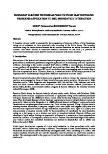
1. Introduction The boundary element method (BEM) is the most potent tool for the solution of linear elliptic partial differential equations (PDEs) in an exterior domain. The standard BEM also serves as an attractive alternative to methods such as the finite-element and finite-difference methods for interior linear elliptic problems. The BEM has thus become an established computational method in recent years (Jaswon and Symm,’ Brebbia,’ Banerjee and Butterfield3). However, apart from suffering the limitation of being inappropriate for nonlinear problems, the BEM is unable to cope directly with discontinuities in the variables in the domain of the PDE. The discontinuity will be assumed to have the topology of a shell-an open surface in three-dimensional problems, a line in two dimensions. An illustration of the general domain is given in Figure 1. The traditional BEM is derived from a boundary integral equation (BIE) formulation of the PDE by dividing the boundary into boundary elements and applying an integral equation method (usually collocation) to obtain the method of solution. For domains in the form of Figure I, the traditional BEM can be applied by dividing the domain into subdomains, as illustrated in Figure 2. Boundary integral equation reformulations of the PDEs on each subdomain can now be obtained and, through coupling these equations across common boundaries, the solution throughout the domain can be obtained. A similar method to the traditional BEM for the solution of a PDE in the infinite domain exterior to a shell discontinuity can be derived through recasting the PDE as an integral equation termed a shelZ integral
method,
discontinuity,
Laplace’s
equation
equation (SIE). A numerical method can then be derived in a way similar to the BEM (see, for example, Ben Mariem and Hamdi4 or Warham’). However, the main value of shell elements is in their use in conjunction with boundary elements. This paper shows how the PDE in the domain of Figure I can be reformulated in a straightforward way as an integral equation termed a boundary and shell integral equation (BSIE) and thus how a numerical method termed the boundary and shell element method (BSEM) can be derived. Boundary element methods have traditionally fallen into two distinct classes, direct BEMs and indirect BEMs, based on direct and indirect integral equation formulations. In this paper direct and indirect BSIE formulations are given for the interior two-dimensional Laplace equation. The BSIEs are a hybrid of the corresponding direct or indirect BIE with the SIE. Hence new integral equation-based methods for the solution of
Address reprint requests to Dr. Kirkup at the Dept. of Mathematics and Computer Science, University of Salford, Salford, UK. Received February
418
7 October 1994
Appl. Math.
1993; revised
Modelling,
24 December
1994,
1993; accepted
Vol. 18, August
2
Figure 1.
Illustration
of the general
0
domain
1994 Butterworth-Heinemann
Boundary
and shell element method:
S. M. Kirkup
can be regarded as hybrids of their respective standard BIE formulations as given, for example, in Jaswon and Symm’ and SIE formulations as given in Ben Mariem and Hamdi4 and Warham.’
jl=\ Figure 2.
Preparation
for application
2’z:~;:;~~z Let the function
v(p) for PES be defined as follows: (PES)
where np is the unit outward normal to S at p. Each shell is assumed to have two sides or surfaces; let I+ be the upper surface and let I_ be the lower surface. The potential cp and its derivatives are generally discontinuous at the shell; however they take limiting values on I+ and I-. Let the functions q+(p), q-(p), v+(p), and u_(p) (pi r) be defined as follows:
of the BEM.
cp+(P) = lim CP(P+ snp), linear elliptic PDEs with discontinuities in its domain are introduced in this paper. The methods are demonstrated on the two-dimensional interior Laplace problem
cp-(P) =
lim
CP(P-
qJ,
E-O+ u+(p) =
lim acp (p + en,), E-O+ an,
V2V4P) = 0 An illustration of the domain is given in Figure 1. It consists of a region D with boundary S and with shell discontinuities I. In order to specify the problem fully, conditions for points on the boundary and on the shell must be stated. These are the boundary condition and the shell condition. Extension of the methods to exterior problems, three-dimensional problems, and to other PDEs is straightforward through the appropriate choice of integral formulation and Green’s function. In Warham,’ the SIEs are derived by first assuming that the shells have finite thickness and hence the standard BIE formulation is valid. The shell thickness is then allowed to approach zero. A similar limiting process can be used to derive the BSIE by assuming S to be fixed and taking the limit as the thickness of the shells approaches zero. The integral equation formulations of the interior Laplace problem are stated in Section 2. In order to derive a particular method, the boundary and shell are divided into uniform elements and the functions defined on the boundary and shell are approximated by a constant on each element. The integral equation method is then derived through collocation. The methods are demonstrated through their application to a test problem where the domain is the unit square and a discontinuity lies between (&i) and ct 1).
u_(p) = lim acp (p - snp) E-O+ an, It is helpful to introduce the functions 6(p), v(p), Q(p), and V(p) for p E I, which are defined as follows: d(p) = V+(P) - C(P) V(P) = V+(P) + V-(P)
In this section the direct and indirect BSIE formulations of the interior Laplace equation are given. The BSIEs
(PEI), (PEI-),
Q(P) = C(P)CP+(P) + (1 - C(P))CP-(P) VP) = c(P)~+(P) - (1 - C(P))=(P)
(PE I-)
The geometrical function c(p) (p E S u r) is defined to be the angle subtended by the points in the interior region at p for points on S and the angle subtended by points in the interior on the face I+ for points on the shell I, each divided by 271.
2.2 Boundary and shell conditions The boundary
condition
has the form
@(P)cp(P) + B(P)U(P) = Y(P)
(P E S)
where a(p), /3(p), and y(p) are functions of p on S. The shell conditions are assumed to have the following general form: a(p)%4
2. Integral equation formulation
(per),
+ ~P)u(P) = f(p)
A(P)@(P) + B(P) V(P) = F(P)
(P E r), (P 6 r)
where a(p), b(p), f(p), A(p), B(p), and F(p) are functions of p on r.
Appl.
Math.
Modelling,
1994,
Vol. 18, August
419
Boundary and shell element method:
S. M. Kirkup
2.3 Integral operator notation The Laplace integral defined as follows: {L&(P)
=
W&(P)
L, M, M’, and N are
on the shell, we have the
Q(P) = {LO),(P) + {M%(P)
G(P, sMs)
sn
=
operators
the boundary S. For points following equations:
n2
d&j
(P, s)ds)
s
VP) = {M’~),(P) + {N%(P)
(P E D u S u I),
dS,
G(P, dAd
- {M’~),(P)
(7)
(PEF) (8)
(P E D CJS TVr)>
V(P) = Ws(P)
(P E S u I),
dS,
(P E I)
The values of q(p) for points in the interior domain are related to the solutions on S and r through the following equation:
4
{M’pL)n(p) = $
- ‘CLu),(p)
+ {M%(P)
- {-W,(P)
(PED)
(9)
P s n
3. Application {N&~(P)
= cp j+n g
(P, q)&)
dS,
(P E S u F)
P
where II c S u F, nq and np are unit outward normal to II when II c S or the unit normal to II, when II c F at q, p and ,u(q) is a bounded function defined for qElI. G(p, q) is the free-space Green’s function for the Laplace equation log r
G(p, q) = - i where r = p -q
in two dimensions
and r = Irl.
2.4 Direct integral equation formulation The equations that make up the BSIE formulation of the Laplace equation are given in this subsection. For points on the boundary the following equation holds: FWMP)
+ C(P)cp(P)
= {W,(P) Equation boundary following
+ W%(P)
- {W,(P)
(PES)
(1)
This section shows how collocation is applied to derive the discrete form of the integral equations. The boundary and shell are divided into uniform elements. The boundary S is divided into n, elements AS,, AS,, . . . , AS,,, the shell F is divided into n, elements Af’r, functions and shell AI-29 . . . , Ar,,, and the boundary functions are approximated by a constant on each element. Let pl, p2,. . . , p., and ql, q2,. . . , q,, be the collocation point with pi~ASi for i = 1,2, . . . , n, and n, and each lying at the center qiEAIi for i= 1,2,..., of the respective element. The boundary is smooth at the collocation points, hence c(p,) = i (i = 1,2,. . . , n,) and c(q,) = f (i = 1, 2,. . , n,). _.. 3.1 Notation It is helpful to introduce Define the vectors of the collocation points as follows:
(1) relates (p(p) and v(p) for points p on the S. For points on the shell, we have the equations:
@(P) = -@f&(P)
+ {W,(P)
- W,(P)
+ W%(P) (2)
(PE f-),
UP) = -{N&(P)
+ (M’~)s(P) + {N%(P)
of collocation
the following notation. function values at the
‘ps = CV(Pl)> cp(P,), . . .2 cp(Pn,)K sr = C&I,), &I& . . . 3&ln,r Vectors v,, gs, as, es, xs, v,, & and _V, are defined similarly. Let the matrices L,,, L,,, Lr,, and L,, be defined as follows:
(3)
CLSSlij = {Le),SJPi)(i
= 1,2,. . . , nd, (j = 1,2, . . . , Q),
The values of q(p) for points in the interior domain are related to the solutions on S and r through the following equation:
CLSrlij = {Le),r,(Pi)(i
= 1,2,. . .,$),(j
- {M+(P)
(P E r)
V(P) = -@W,(P)
CLrrlij (4)
(P E D)
The equations that make up the indirect BSIE formulation of the Helmholtz equation are given in this subsection. For points on the boundary the following equations hold: + {M%(P)
- {LUMP)
U(P) = {M’&(P) + c(P~(P) + {N%(P) - (bf’U~r(D~ CDE sj I
,1
\*
I
\_
I
(P E S)
(5) (6)
where 0 is generally known as a source density function. Equations (5) and (6) relate q(p) and u(p) for points p on
420
Appl.
Math.
Modelling,
1994,
= {Le},r,(qi)
, n,),
G = 1,X. . , n,), (j = 1,2,. . , nd
where e is the unit function. Notation for the other integral operators (M, M’, and N) is developed in a similar way.
2.5 Indirect integral equation formulation
V(P) = {La),(p)
CL,Slij = {Le},3S,(%)(i = 1,Z. . . ,4-L (j = I,&.
+ {JWs(P) + {M%(P)
- {Wr(P)
= L2,. . .,Q),
Vol. 18, August
3.2 Discrete form of the integral equations The adoption of the notation above allows us to construct the following linear systems of approximations, which are the discrete analogues of the direct integral equation formulation (lH3): CM,,
+
+Issl~s
- LSSE.Y+ WI-~,
- Ls,vr~
(10)
Q = --M,s’~s _r
+ Lrs+s + WI-6,
- Lrrvr,
(11)
V = -N,sW, _r
+ WSE.T + Nrr6,
- W-,V~,
(12)
Boundary and shell element method: Similarly, the discrete form of the indirect equation formulation (SHS) is as follows: -cps = LSLLS + MS,&
+ Ns&
+ M,&
-
(14)
M:rvr>
- Lrrvr,
(15)
- M;rvr
(16)
Fr = M’,sos + N,,&The boundary following form
(13)
- Lsrlir,
XV= CMSs + :Issl~s CD r = Lrsos
integral
condition
can
be
written
in
the (17)
D;S(PS + D&us = 1/s
where D& = diag(sr,, x2, . , c(,,,)and Dgs = diag(P,, p2, . . , &,J. Similar equations can be obtained for the shell condltlon.
Kirkup. These numerical integrations are computed to sufficient accuracy so the error does not contribute significantly to the overall error in the integral equation methods. 4.1 Direct BSEM The following linear system of equations approximations (lOH12) and (17):
Wss + &s) % M,, N,s I
- Ls D$ -L,s -ML
Os, -&IOx Os, I,, -I%,Or,- -N,, I[
& G &, 8, 1
= 1s 0 _l_I;I0
(18)
On solution the approximations &, &, &-, & to qs, h, &, and 6, are obtained. The discrete form of equation (4) is then used to compute the solution in the domain D. Results from the application of the method to the test problem are given in Table 1. The solution is sought at the points (0.25, 0.25), (0.25, 0.5), and (0.25, 0.75) in the domain with 9 (8 boundary and 1 shell), 18 (16 + 2), 36 (32 + 4), 72 (64 + 8), 144 (128 + 16), 288 (256 + 32), and 576 (512 + 64) uniform elements. Thus the element lengths h are 4, 4, 4, &, A, 8, and &, respectively.
p=-1
cp=l
4.2 Indirect BSEM
(191)
:o, 1)
The following linear system of equations equations (13)-(17),
v=o .
1 SS
v=o
v=o
follows from
0 _s
4. Application of the BSEMs to the test problem To demonstrate the direct and indirect BSEMs, the test problem with the domain of the unit square and with a discontinuity between ($4) and (3, 1) is introduced. The boundary conditions are such that q(p) = 1 for 0 < p1