ture associated with the measurement data, providing solution algorithms for the main types of .... Experimental data analysis is a key activity in metrology.
NPL Report CMSC 24/03
Report to the National Measurement System Directorate, Department of Trade and Industry From the Software Support for Metrology Programme
The classification and solution of regression problems for calibration
By M G Cox, A B Forbes, P M Harris and I M Smith
Revised August 2004
The classification and solution of regression problems for calibration
M G Cox, A B Forbes, P M Harris and I M Smith Centre for Mathematics and Scientific Computing
Revised August 2004
ABSTRACT Many experiments in metrology involve the use of instruments or measuring systems that measure values of a response variable corresponding to given values of a stimulus variable. The calibration of such instruments requires using a set of measurements of stimulus and response variables, along with their associated uncertainties, to determine estimates of the parameters that best describe the relationship between them, along with their associated uncertainty matrix. Algorithms for determining the calibration parameters for problems where measurements of the stimulus variable can be assumed to be accurate relative to those of the response variable are well known. However, there is much less awareness in the metrology community of solution algorithms for more generalised problems. Many standards that deal with calibration, while identifying the types of regression problems to be solved, offer only limited advice regarding the selection and use of solution algorithms. There is also a need for guidance regarding uncertainty evaluation. The aim of this report is to provide more assistance to the metrologist, allowing the calibration problem to be easily classified according to the uncertainty structure associated with the measurement data, providing solution algorithms for the main types of calibration problems, and describing the evaluation of uncertainties associated with the calibration parameters. The report will also act as input to JCGM-WG1 and ISO TC69/SC6/WG7.
c Crown copyright 2004
Reproduced by permission of the Controller of HMSO
ISSN 1471–0005
Extracts from this report may be reproduced provided the source is acknowledged and the extract is not taken out of context
Authorised by Dr Dave Rayner, Head of the Centre for Mathematics and Scientific Computing
National Physical Laboratory, Queens Road, Teddington, Middlesex, United Kingdom TW11 0LW
Contents 1
Introduction
1
2
Terms and definitions
3
3
Problem formulation 3.1 Functional models . . . . . . . . . . . . . . . . . . . . . . . . . . 3.2 Least squares analysis/adjustment . . . . . . . . . . . . . . . . . 3.3 Uncertainty models . . . . . . . . . . . . . . . . . . . . . . . . .
5 5 6 7
4
Linear models 4.1 Linear diagonally weighted least squares problems . . . 4.1.1 Solution algorithm . . . . . . . . . . . . . . . . 4.1.2 Uncertainties associated with solution parameters 4.2 Linear Gauss-Markov regression problems . . . . . . . . 4.2.1 Solution algorithms . . . . . . . . . . . . . . . . 4.2.2 Uncertainties associated with solution parameters
. . . . . .
. . . . . .
. . . . . .
. . . . . .
. . . . . .
12 12 13 13 13 14 15
Non-linear models 5.1 Non-linear diagonally weighted least squares problems . 5.1.1 Solution algorithm . . . . . . . . . . . . . . . . 5.1.2 Uncertainties associated with solution parameters 5.2 Non-linear Gauss-Markov regression problems . . . . . 5.2.1 Solution algorithms . . . . . . . . . . . . . . . . 5.2.2 Uncertainties associated with solution parameters 5.3 Generalised distance regression problems . . . . . . . . 5.3.1 Solution algorithm . . . . . . . . . . . . . . . . 5.3.2 Uncertainties associated with solution parameters 5.4 Generalised Gauss-Markov regression problems . . . . . 5.4.1 Solution algorithm . . . . . . . . . . . . . . . . 5.4.2 Uncertainties associated with solution parameters
. . . . . . . . . . . .
. . . . . . . . . . . .
. . . . . . . . . . . .
. . . . . . . . . . . .
. . . . . . . . . . . .
16 16 16 17 17 18 19 19 20 22 22 22 24
Applications of the calibration curve 6.1 Function evaluation . . . . . . . . . . . . . . . 6.1.1 Linear models . . . . . . . . . . . . . . 6.1.2 Non-linear models . . . . . . . . . . . 6.2 Inverse function evaluation . . . . . . . . . . . 6.3 Derived quantities . . . . . . . . . . . . . . . . 6.3.1 Linear functions of the parameters . . . 6.3.2 Non-linear functions of the parameters .
. . . . . . .
. . . . . . .
. . . . . . .
. . . . . . .
. . . . . . .
25 25 25 26 26 27 27 28
7 Polynomial calibration curves 7.1 Straight line calibration curves . . . . . . . . . . . . . . . . . . .
29 30
5
6
i
. . . . . . .
. . . . . . .
. . . . . . .
. . . . . . .
. . . . . . .
8
Summary
32
9
Acknowledgements
33
A Generalised QR factorisation
36
B Gauss-Newton algorithm
38
C Bisection algorithm
39
D Derivation of expressions for uncertainty evaluation D.1 Linear diagonally weighted least squares problems D.2 Linear Gauss-Markov regression problems . . . . . D.3 Generalised distance regression problems . . . . . D.4 Generalised Gauss-Markov regression problems . .
ii
. . . .
. . . .
. . . .
. . . .
. . . .
. . . .
. . . .
. . . .
40 40 40 42 44
NPL Report CMSC 24/03
1
Introduction
Experimental data analysis is a key activity in metrology. It involves developing a mathematical model of a physical system in terms of mathematical equations involving parameters that describe all relevant aspects of the system. The model specifies how the system is expected to respond to input data and the nature of the uncertainties associated with this data. Given measured data, estimates of the model parameters are determined by solving the mathematical equations constructed as part of the model, and this requires developing an algorithm (or estimator) to determine values for the parameters that best explain the data. In many areas of metrology the relationship between a “stimulus” variable and a “response” variable is used as the basis for the calibration of an instrument or measuring system. Actual measurements consisting of the observed response for settings of the stimulus variable are fitted by an appropriate calibration curve to quantify the required relationship. In cases where the measurements of the stimulus variable can be considered to be accurate compared with those of the response variable, ordinary least squares or other procedures can be used to provide the “regression” curve. The uncertainties associated with the curve and its subsequent usage can also readily be determined. However, in many applications, such as dimensional metrology, gas-standards work and analytical chemistry, the uncertainties associated with the measurements of the stimulus variable can be appreciable, and ignoring them can yield invalid results and unreliable uncertainties associated with the calibration curve. The motivation for this report is as follows: • Calibration problems occur widely in metrology and algorithms for problems where measurements of the stimulus variable can be assumed to be accurate relative to those of the response variable are well known. However, there is much less awareness in the metrology community of solution algorithms for more generalised problems and this lack of awareness needs to be addressed. • A recent Software Support for Metrology (SSfM) survey [17] has investigated the extent to which metrology algorithms are used within standards. This survey has identified the need for more comprehensive advice regarding the selection and use of such algorithms. For example, there is a generic standard [8] on regression, but it has a limited scope, dealing only with straight line calibration curves. Also identified is the need for more guidance regarding uncertainty evaluation and a recommendation that reliable software be provided. The survey identifies the requirement for generic standards that specify the statistical methods that should be used in all the calibration cases that occur in metrology, with appropriate guidance on uncertainty evaluation. http://www.npl.co.uk/ssfm/download/documents/cmsc24 03.pdf
Page 1 of 46
NPL Report CMSC 24/03
• NPL has representation on JCGM-WG11 and ISO TC69/SC6/WG72 , both of which have identified a need for increased guidance relating to calibration problems. In the case of JCGM-WG1, it is expected that guidance will be provided in the form of a supplemental guide to the GUM [3] on least squares adjustment. The main aims of this report are therefore: • To describe the main types of uncertainty models encountered by metrologists, and provide a basic classification of the resulting calibration problems into which metrologists can characterise their own problems. • To provide algorithms for the estimation of calibration parameters and their associated uncertainties. • To describe the “application” of the calibration curve to the evaluation of other quantities and their associated uncertainties. • To act as input to the work of JCGM-WG1 and ISO TC69/SC6/WG7. The layout of the remainder of this report is as follows. Section 2 introduces many of the relevant terms and the mathematical notation. Section 3 describes the formulation of the calibration problem and introduces a classification of calibration problems based on the structure of the uncertainty matrix associated with the stimulus and response variables. Sections 4 and 5 describe algorithms for estimating the calibration curve parameters and their associated uncertainties when the response variable is respectively a linear function and a non-linear function of the stimulus variable. In both these sections, it is shown that the calibration problems require the solution of a number of “standard” problems to which standard algorithmic tools can be applied. In section 6, the application of the calibration curve to function evaluation, inverse function evaluation and the evaluation of other derived quantities is detailed. Section 7 discusses some of the issues concerning polynomial calibration curves, a class of calibration curve widely used in metrology. Concluding remarks are given in Section 8. August 2004 revision This revised version of the report contains corrections to formulæ concerning Chebyshev polynomials in section 7.1.
1
Joint Committee for Guides in Metrology, Working group 1 (Measurement Uncertainty) Technical committee 69/Subcommittee 6/Working group 7 (Application of statistical methods/Measurement methods and results/Uncertainty of measurement) 2
Page 2 of 46
http://www.npl.co.uk/ssfm/download/documents/cmsc24 03.pdf
NPL Report CMSC 24/03
2
Terms and definitions
Throughout the report, the following notation is used: m n
number of measurements. number of model parameters. a1 .. vector of model parameters a = . . an set of m elements indexed by i = 1, . . . , m. transpose of a vector or matrix. zero matrix. identity matrix. α β . diagonal matrix .. .
a {xi }m 1 aT , A T 0 I diag{α, β, . . . , ω}
ω
kak m X
xi i=1 ∂h ∂t (t0 ) ∂h ∂aj (a0 ) ∂h ∂t (t0 , a0 ) ∂h ∂aj (t0 , a0 )
∇a h(a0 )
the 2-norm of the vector a: kak = a21 + · · · + a2n sum of elements of the vector x:
m X
�1 2
.
xi = x1 + · · · + xm .
i=1
partial derivative of the function h = h(t) with respect to t, evaluated at t = t0 . partial derivative of the function h = h(a) with respect to aj , evaluated at a = a0 . partial derivative of the function h = h(t, a) with respect to t, evaluated at t = t0 , a = a0 . partial derivative of the function h = h(t, a) with respect to aj , evaluated at t = t0 , a = a0 . vector of partial derivatives of the function h = h(a) with respect to the parameters at a = a0 : ∂ha, evaluated (a0 ) ∂a1 . . .. ∇a h(a0 ) = ∂h ∂an (a0 )
http://www.npl.co.uk/ssfm/download/documents/cmsc24 03.pdf
Page 3 of 46
NPL Report CMSC 24/03
∇a h(t0 , a0 )
vector of partial derivatives of the function h = h(t, a) with respect to the parameters a, evaluated at t = t0 , a = a0 : ∂h (t0 , a0 ) ∂a1 . . .. ∇a h(t0 , a0 ) = ∂h ∂an (t0 , a0 )
J ux var(x) cov(x, y) U (or Ua )
Page 4 of 46
Jacobian matrix associated with a set of functions {hi (a)}m 1 of ∂hi parameters a with general element Jij = ∂a . j standard uncertainty associated with the estimate x of random variable X. variance associated with the estimate x of random variable X: var(x) = u2x . covariance associated with the estimates x and y of random variables X and Y . Note: cov(x, x) = var(x). uncertainty matrix (also known as covariance matrix) associated with a having general element Uij = Ua,ij = cov(ai , aj ) if i 6= j, Uij = Ua,ij = var(ai ) if i = j.
http://www.npl.co.uk/ssfm/download/documents/cmsc24 03.pdf
NPL Report CMSC 24/03
3 3.1
Problem formulation Functional models
Many metrology experiments involve determining the behaviour of a response variable v as a function of a stimulus variable t. Model building involves establishing the functional relationship between these quantities, usually involving a set of model parameters a1 a = ... , an i.e., v = h(t, a).
(1)
The terms a parametrize the range of possible response behaviour, and the actual behaviour is specified by determining values for these parameters from measurement data. Equation (1) defines a calibration curve and a is sometimes referred to as the vector of calibration coefficients. The functional model is linear (in the parameters a) if h can be expressed in the form h(t, a) =
n X
aj hj (t) = a1 h1 (t) + a2 h2 (t) + · · · + an hn (t),
j=1
where {hj (t)}n1 is a set of basis functions, and is non-linear otherwise. Often the same curve can be expressed in a number of ways by choosing different basis functions. The problem of choosing an appropriate set of basis functions to represent the calibration curve is one of parametrisation; a fuller discussion is available [7]. Section 7 contains a brief discussion of parametrisation issues that arise when working with polynomials which constitute a class of calibration curves widely used in metrology.
Example: Calibration of a thermometer. The response v of a thermometer to temperature t is modelled as v = a1 + a2 (t − t0 ), where t0 is a fixed temperature. This is a linear calibration curve with basis functions h1 (t) = 1, h2 (t) = t − t0 and
"
a=
a1 a2
#
.
http://www.npl.co.uk/ssfm/download/documents/cmsc24 03.pdf
Page 5 of 46
NPL Report CMSC 24/03
]
Example: Calibration of a hydrophone. As part of the calibration of an underwater electroacoustic transducer, measurements are made of the response of the transducer to a sinusoidal drive signal of frequency f . Assuming that the system behaves as a linear damped harmonic oscillator, the response v is modelled as a function of time as follows: v = A1 sin(2πf t + φ1 ) +
1+n Xr
Ak edk t sin(2πfk t + φk ),
k=2
where the first term represents the steady-state behaviour of the device, and the remaining terms are used to represent its resonant behaviour. The coefficients r r a comprise the amplitudes {Ak }1+n , resonant frequencies {fk }2+n , damping 1 2 2+nr 2+nr factors {dk }2 and phase angles {φk }1 . The calibration curve is a non-linear function of the coefficients a. ]
3.2
Least squares analysis/adjustment
In this section, we describe the general approach to the least squares analysis or adjustment (LSA) of calibration data. Suppose, in a calibration of a measurement system, that the response of the system is modelled as v = h(t, a) and that measurements " # v x= , t comprising of measurements v1 .. v = . and t = vm
t1 .. .
tm
of the response and stimulus variables, are gathered. Associated with x is its uncertainty matrix Ux , a 2m × 2m symmetric matrix. Suppose Ux can be factored as Ux = GGT , where G is an 2m × k matrix. G could be derived from an eigenvalue decomposition of Ux , for example, but often the nature of the experiment provides Ux in Page 6 of 46
http://www.npl.co.uk/ssfm/download/documents/cmsc24 03.pdf
NPL Report CMSC 24/03
this form. In a least squares analysis, estimates of the calibration parameters a are determined by solving the optimisation problem min yT y
(2)
a,q,y
subject to the constraints "
v t
#
"
=
h(q, a) q
#
+ Gy,
(3)
where the ith element of the m-vector h(q, a) is h(qi , a). This optimisation problem implicitly defines a = a(x) as a function of the input data x and the general principles of the GUM [8] can be applied to determine the uncertainty matrix Ua associated with a, given the uncertainty matrix Ux . LSA methods are used widely throughout metrology (and science in general) and can be justified for a wide range of applications. For measurement data modelled in terms of Gaussian distributions, the LSA estimate of the parameters a provides the most likely explanation of the data, i.e., the maximum likelihood estimate. The Gauss Markov theorem [13] states that, with some mild qualifications, the LSA approach makes the best use of the available data x and Ux . While (2) defines the LSA estimate in completely general terms, in many regression problems the uncertainty matrix Ux has a structure that allows the optimisation problem to be reformulated in a more simple way. In this report, we list some of the most common uncertainty structures and describe corresponding estimation algorithms. The algorithms employ numerically stable procedures such as orthogonal factorisation methods in order to avoid the unnecessary loss of accuracy in the computed estimates. The LSA method assumes that the data uncertainty matrix Ux is known. However, ˜ for data x and Ux is the same as that for x and σ 2 Ux , σ 2 > 0, i.e., the solution a ˜. In this way, LSA changing Ux by a scale factor does not change the solution a 2 T methods can be applied to data x and Ux = σ GG , where the factor G is known but the scale σ 2 is unknown. In this situation, the uncertainty matrix Ua˜ associated with the estimated parameters can be written as Ua˜ = σ 2 U U T , ˜ has been determined, an where U is known. Often, once the LSA estimate a estimate σ ˆ of σ can be derived and then used to specify Ua˜ and Ux completely.
3.3
Uncertainty models
The uncertainties associated with the measurement data "
x=
v t
#
http://www.npl.co.uk/ssfm/download/documents/cmsc24 03.pdf
Page 7 of 46
NPL Report CMSC 24/03
are described by the uncertainty matrix "
Ux =
Uv Uvt T Uvt Ut
#
.
The ith diagonal element of sub-matrix Ut [Uv ] is var(ti ) [var(vi )], the variance of ti [vi ], while the i, j (i 6= j) element of Ut [Uv ] is cov(ti , tj ) [cov(vi , vj )], the covariance of ti and tj [vi and vj ]. The sub-matrix Uvt contains the covariance of the stimulus and response variables, i.e., the i, j element of Uvt is cov(vi , tj ). Common examples of calibration problems where the measurements of the stimulus variable are assumed to be accurate relative to the measurements of the response variable are those where the measurements of the response variable are: 1. uncorrelated but have unknown equal variances s2 , i.e., Uv = s2 I with s unknown, 2. uncorrelated but have known equal variances σ 2 , i.e., Uv = σ 2 I with σ known, 3. uncorrelated with the ith measurement having known variance σi2 , i.e., Uv = 2 }, diag{σ12 , . . . , σm 4. correlated with general uncertainty matrix Uv , while typical examples of more generalised uncertainty structures include cases where: 5. the measurements are uncorrelated but the measurements of the stimulus and response variables have unknown equal variances r2 and s2 , respectively, but the ratio of r to s is known, i.e., Ut = r2 I, Uv = s2 I, Uvt = 0, rs = α known, 6. the measurements are uncorrelated and the measurements of the stimulus and response variables have known equal variances ρ2 and σ 2 , respectively, i.e., Ut = ρ2 I, Uv = σ 2 I, Uvt = 0, 7. the measurements are uncorrelated and the ith measurements of the stimulus and response variables have known variances ρ2i and σi2 respectively, i.e., 2 }, U Ut = diag{ρ21 , . . . , ρ2m }, Uv = diag{σ12 , . . . , σm vt = 0, 8. as 7, but the ith measurements ti and vi are correlated with known covariance 2 }, cov(vi , ti ) = αi , i.e., Ut = diag{ρ21 , . . . , ρ2m }, Uv = diag{σ12 , . . . , σm Uvt = diag{α1 , . . . , αm }, Page 8 of 46
http://www.npl.co.uk/ssfm/download/documents/cmsc24 03.pdf
NPL Report CMSC 24/03
9. all the response variable measurements are (generally) correlated with known uncertainty matrix Uv , all the stimulus variable measurements are (generally) correlated with known uncertainty matrix Ut and there is no correlation between stimulus and response variable measurements, i.e., Uvt = 0, 10. all the measurements are (generally) correlated with known uncertainty matrix Ux . Note that any uncertainty model can be considered to belong to at least one of types 3, 4, 8 or 10. In particular, any uncertainty model can be classified as the most general (case 10), but the provision of information to it, and its numerical handling, will not necessarily be efficient. The above list is not exhaustive and it is not the intention of this report to provide individual solution algorithms for each. In the following sections we will focus on the four distinct types of statistical model that we consider to be the most important, viz., 3, 4, 8 and 10. Algorithms for each of the resulting calibration problems, namely [9]: I. diagonally weighted least squares problems (uncertainty models 1, 2 and 3), i.e., Uv diagonal, Ut = Uvt = 0, II. Gauss-Markov regression problems (uncertainty model 4), i.e., Ut = Uvt = 0, III. generalised distance regression problems (uncertainty models 5, 6, 7 and 8) [2], i.e., Uv , Ut and Uvt diagonal, IV. generalised Gauss-Markov regression problems (uncertainty models 9 and 10), i.e., Ux a full matrix, are described along with details of the evaluation of the uncertainties associated with the solutions to these problems. Note that while the same algorithm is therefore used to find parameter estimates for uncertainty model 1 (5) as for uncertainty models 2 and 3 (6, 7 and 8), evaluation of the uncertainty matrix associated with the solution parameters requires an estimate of the unknown variance(s) to be incorporated; see, for example, [7]. Table 1 relates the four main types of calibration problem listed above to the appropriate parts of Sections 4 and 5. For calibration problems of types I and II, direct methods are used to obtain the solution parameters, and different algorithms are recommended for the cases where the calibration function h is linear and non-linear. For calibration problems of http://www.npl.co.uk/ssfm/download/documents/cmsc24 03.pdf
Page 9 of 46
NPL Report CMSC 24/03
Calibration problem I I II II III III IV IV
Calibration function Linear Non-linear Linear Non-linear Linear Non-linear Linear Non-linear
Section 4.1 5.1 4.2 5.2 5.3 5.3 5.4 5.4
Table 1: Location in this report of descriptions of solution algorithms corresponding to the four main types of calibration problem, for linear and non-linear calibration functions.
types III and IV, where non-direct methods involving the application of the GaussNewton algorithm [11] are recommended, there is no clear advantage in distinguishing between linear and non-linear calibration functions.
Example: Preparation of primary standard natural gas mixtures Within the Centre for Optical and Analytical Measurement at NPL, one part of the work of the Environmental Standards Group is to prepare primary standard natural gas mixtures. Cylinders containing natural gas are prepared gravimetrically to contain known compositions of each of the 11 constituent components (methane, ethane, propane, l-butane, n-butane, l-pentane, n-pentane, neo-pentane, hexane, nitrogen and carbon dioxide). Mixtures are prepared to cover various concentration ranges, e.g., methane: 64% − 98%. These primary standard mixtures are used as the basis for determining the composition of a new mixture and hence its calorific value. Given a number of primary standard natural gas mixtures containing known concentrations of one of the constituent components (e.g., CO2 ), the detector response for each mixture and the detector response for the new mixture, it is required to determine the concentration of CO2 in the new mixture. An approach to solving this problem is firstly to use the calibration data (relating to the primary gas mixtures) to calibrate the detector and, secondly, to use the calibration curve so constructed with the new measurement to predict the concentration in the new mixture. Uncertainties to be accounted for are: • the process of preparing the primary standards means that they are known inexactly, and indeed the uncertainties in the standards may be correlated Page 10 of 46
http://www.npl.co.uk/ssfm/download/documents/cmsc24 03.pdf
NPL Report CMSC 24/03
5
8
x 10
Detector reponse (peak area)
7 6 5 4 3 2 1 0 −1 −1
0
1
2
3 4 5 CO2 concentration (%)
6
7
8
Figure 1: Sample data (+), fitted calibration curve and predicted measurement (◦).
(this is a consequence of the gravimetric process used to prepare the standard mixtures which involves comparing on a balance each standard mixture at each stage of preparation against calibrated masses selected from a common set of masses), • the data returned by the detector (which is based on the analytical technique of chromatography) is subject to measurement uncertainty. The data analysis has to account for the inexactness of the measurement data and quantify the resulting uncertainty associated with the final measurement result. Figure 1 shows a sample set of measurement data, with the ellipses around the calibration points illustrating the uncertainties in the concentrations and detector responses. (The uncertainty ellipses have been magnified greatly for illustrative purposes.) The figure also shows a linear calibration curve which is used to estimate the concentration of the component for which the detector response (and its uncertainty) is known. Note that of the ten models described earlier in this section, this example is classified as uncertainty model 9 (and the resulting calibration problem therefore is classified as type IV). ] http://www.npl.co.uk/ssfm/download/documents/cmsc24 03.pdf
Page 11 of 46
NPL Report CMSC 24/03
4
Linear models
In this section, we assume that the calibration function is linear in the parameters a, i.e., h(ti , a) =
n X
aj hj (ti ),
j=1
and define C to be the m × n matrix whose ith row is cT i , where h1 (ti ) .. ci = . . hn (ti )
4.1
Linear diagonally weighted least squares problems
Consider the case where the measurements {ti }m 1 of the stimulus variable are assumed to be accurate relative to the measurements {vi }m 1 of the response variable, the response variable measurements being uncorrelated and therefore having (diagonal) uncertainty matrix 2 Uv = diag{σ12 , . . . , σm }, σi > 0.
The LSA problem is min (h(t, a) − v)T Uv−1 (h(t, a) − v) . a
The matrix Uv can be written as Uv = LLT , where L = diag{σ1 , . . . , σm }. ˜ = L−1 v, the LSA problem takes the form of a (weighted) Setting C˜ = L−1 C and v linear least squares problem, and estimates of a are found by solving min a
�
˜ −v ˜ Ca
�T �
�
˜ −v ˜ , Ca
i.e., ˜ −v ˜ k2 . min kCa a
Page 12 of 46
http://www.npl.co.uk/ssfm/download/documents/cmsc24 03.pdf
NPL Report CMSC 24/03
4.1.1 Solution algorithm For reasons of numerical stability and efficiency, the use of orthogonal factorisation is generally recommended to solve this problem. The matrix C˜ has QR factorisation [12] " # ˜ R ˜ C˜ = Q , (4) 0 ˜ is m × m orthogonal, i.e., Q ˜ TQ ˜ = I, the m × m identity matrix, and R ˜ where Q is n × n upper-triangular. ˜ T xk = kxk, we have Using the fact that kQ
" # " #
˜
˜ q R
1 ˜ −v ˜ −Q v ˜ k = kQ Ca ˜k = kCa a−
,
0 ˜2 q
˜T
˜T
˜ Tv ˜ . From this it is seen ˜ 1 is the first n and q ˜ 2 the last m − n elements of Q where q ˜ −v ˜ k is minimised if a solves the upper-triangular system that kCa ˜ =q ˜1. Ra ˜ can be calculated efficiently from C and v by row scaling: C˜ and v ˜i = c
vi ci , v˜i = . σi σi
4.1.2 Uncertainties associated with solution parameters ˜, is given by Ua˜ , the uncertainty matrix associated with the solution parameters a [13] Ua˜ = U U T , where U is the solution of the upper-triangular system ˜ = I. RU A fuller derivation of this expression can be found in Appendix D.
4.2
Linear Gauss-Markov regression problems
Consider the case where the measurements {ti }m 1 of the stimulus variable are assumed to be accurate relative to the measurements {vi }m 1 of the response variable, the response variable measurements being correlated and therefore having (general) uncertainty matrix Uv with rank(Uv ) = m. http://www.npl.co.uk/ssfm/download/documents/cmsc24 03.pdf
Page 13 of 46
NPL Report CMSC 24/03
The LSA problem is min (h(t, a) − v)T Uv−1 (h(t, a) − v) , a
and takes the form of a linear Gauss-Markov regression problem, with estimates of a found by solving min (Ca − v)T Uv−1 (Ca − v). a
4.2.1
Solution algorithms
The Gauss-Markov estimate can be found by forming the Cholesky decomposition [12] of Uv , Uv = LLT , where L is m × m lower-triangular, and then solving
2
˜
˜ , −v min Ca
(5)
a
˜ solve the upper-triangular systems where C˜ and v LC˜ = C, L˜ v = v. This problem can be solved using the approach described in section 4.1.1. However, if Uv is poorly conditioned (a consequence of strong correlation effects) ˜ may introduce significant numerical instability. the formation of C˜ and v A stable approach to solving this type of problem is provided by generalised QR factorisation. This section will list the main points in the application of this method. More details can be found in Appendix A. Evaluate the generalised QR factorisation of the pair (C, L), i.e., find m × m orthogonal matrix Q, n × n upper-triangular matrix R, m × m upper-triangular matrix T and m × m orthogonal matrix Z such that "
C=Q
R 0
#
, QT L = T Z.
Partition Q and T : Q=
h
Q1 Q2
i
"
, T =
T11 T12 0 T22
#
,
where Q1 , Q2 , T11 , T12 and T22 are respectively m × n, m × (m − n), n × n upper-triangular, n × (m − n) and (m − n) × (m − n) upper-triangular. Page 14 of 46
http://www.npl.co.uk/ssfm/download/documents/cmsc24 03.pdf
NPL Report CMSC 24/03 Let (m − n) × (m − n) matrix T˜22 be the solution of the upper-triangular system T22 T˜22 = I. ˜ are then given by the solution of the upper-triangular The solution parameters a system � � ˜22 QT v. T − T R˜ a = QT 12 2 1 The generalised QR factorisation can also be applied in the case where Uv is not full rank, but we do not consider this case further here.
4.2.2 Uncertainties associated with solution parameters ˜, is given by Ua˜ , the uncertainty matrix associated with the solution parameters a Ua˜ = U U T , where U is the solution of the upper-triangular system RU = T11 . A fuller derivation of this expression can be found in Appendix D.
http://www.npl.co.uk/ssfm/download/documents/cmsc24 03.pdf
Page 15 of 46
NPL Report CMSC 24/03
5
Non-linear models
5.1
Non-linear diagonally weighted least squares problems
Consider the case where the measurements {ti }m 1 of the stimulus variable are assumed to be accurate relative to the measurements {vi }m 1 of the response variable, the response variable measurements being uncorrelated and therefore having associated uncertainty matrix 2 Uv = diag{σ12 , . . . , σm }, σi > 0.
The LSA problem is min (h(t, a) − v)T Uv−1 (h(t, a) − v) . a
If the calibration function is non-linear in the parameters a, then the above LSA problem takes the form of a weighted non-linear least squares problem, and estimates of the parameters a can be found by solving min a
where
5.1.1
m X
f˜i2 (a),
(6)
i=1
h(ti , a) − vi f˜i (a) = . σi Solution algorithm
Let
f˜1 (a) .. ˜f (a) = . . f˜m (a)
Then the minimisation problem (6) can be written as min ˜f T (a)˜f (a). a
Estimates of the solution parameters can be found by applying the Gauss-Newton algorithm (see Appendix B) to ˜f (a). At each iteration of the Gauss-Newton algorithm we are required to solve, in the least squares sense, ˜ = −˜f , Jp Page 16 of 46
http://www.npl.co.uk/ssfm/download/documents/cmsc24 03.pdf
NPL Report CMSC 24/03 where J˜ is the m × n Jacobian matrix associated with ˜f , evaluated at the current b of the solution parameters. estimate a b + p. An updated estimate of the calibration curve parameters is now given by a
5.1.2 Uncertainties associated with solution parameters ˜, is given by Ua˜ , the uncertainty matrix associated with the solution parameters a �−1
�
Ua˜ = J˜T J˜
,
where J˜ is the m × n Jacobian matrix associated with ˜f (˜ a). Let J˜ have QR factorisation "
˜ J˜ = Q
˜ R 0
#
,
˜ is m × m orthogonal and R ˜ is n × n upper-triangular. where Q Since ˜ T R, ˜ J˜T J˜ = R Ua˜ is given by Ua˜ = U U T , where U is the solution of the upper-triangular system ˜ = I. RU
5.2
Non-linear Gauss-Markov regression problems
Consider the case where the measurements {ti }m 1 of the stimulus variable are assumed to be accurate relative to the measurements {vi }m 1 of the response variable, the response variable measurements being correlated and therefore having associated uncertainty matrix Uv with rank(Uv ) = m. The LSA problem is min (h(t, a) − v)T Uv−1 (h(t, a) − v) . a
If the calibration function is non-linear in the parameters a, then the above LSA problem takes the form of a non-linear Gauss-Markov problem, and estimates of the parameters a can be found by solving min f (a)T Uv−1 f (a), a
http://www.npl.co.uk/ssfm/download/documents/cmsc24 03.pdf
(7) Page 17 of 46
NPL Report CMSC 24/03
where h(t1 , a) − v1 f1 (a) .. . .. f (a) = . = . h(tm , a) − vm fm (a)
5.2.1
Solution algorithms
Calculate the Cholesky factorisation Uv = LLT , where L is m×m lower-triangular, and let L˜f (a) = f (a). Then the minimisation problem (7) can be written as min ˜f T (a)˜f (a). a
Estimates of the solution parameters can be found by applying the Gauss-Newton algorithm (see Appendix B) to ˜f (a). At each iteration of the Gauss-Newton algorithm we are required to solve, in the least squares sense, ˜ = −˜f , LJ˜ = J, Jp where J is the m × n Jacobian matrix associated with f , evaluated at the current b of the solution parameters. estimate a As in the linear case, if L is well conditioned this represents a satisfactory approach to solving (7). Otherwise, the formation of J˜ and ˜f can introduce numerical instability. A stable approach to finding the update step is provided by generalised QR factorisation. This section will list here only the main points in the application of this method. More details can be found in Appendix A. Evaluate the generalised QR factorisation of the pair (J, L), i.e., find m × m orthogonal matrix Q, n × n upper-triangular matrix R, m × m upper-triangular matrix T and m × m orthogonal matrix Z such that "
J =Q
R 0
#
, QT L = T Z.
Partition Q and T : Q= Page 18 of 46
h
Q1 Q2
i
"
, T =
T11 T12 0 T22
#
,
http://www.npl.co.uk/ssfm/download/documents/cmsc24 03.pdf
NPL Report CMSC 24/03
where Q1 , Q2 , T11 , T12 and T22 are respectively m × n, m × (m − n), n × n upper-triangular, n × (m − n) and (m − n) × (m − n) upper-triangular. Let (m − n) × (m − n) matrix T˜22 be the solution of the upper-triangular system T22 T˜22 = I. The Gauss-Newton step p is then given by the solution of the upper-triangular system � � Rp = T12 T˜22 QT − QT f . 2
1
b + p. An updated estimate of the calibration curve parameters is now given by a
We note that, unlike the linear case in Section 4.2, the case where Uv is not full rank cannot in general be solved using the Gauss-Newton algorithm and generalised QR factorisation since the optimisation problem involves non-linear constraints.
5.2.2 Uncertainties associated with solution parameters ˜ is given by Ua˜ , the uncertainty matrix associated with the solution parameters a �
�−1
Ua˜ = J˜T J˜
,
where LJ˜ = J, J being the Jacobian matrix evaluated at the solution parameters ˜. a A similar analysis to that carried out in Section 4.2.2 (see also Appendix D for a fuller derivation) gives Ua˜ = U U T , where U is the solution of the upper-triangular problem RU = T11 .
5.3
Generalised distance regression problems
Consider the case where the the stimulus variable measurements are uncorrelated and have uncertainty matrix Ut = diag{ρ21 , . . . , ρ2m }, the response variable mea2 } surements are uncorrelated and have uncertainty matrix Uv = diag{σ12 , . . . , σm and the ith measurements ti and vi are correlated with cov(vi , ti ) = αi , i.e., Uvt = diag{α1 , . . . , αm }, σi2 ρ2i − αi2 6= 0. http://www.npl.co.uk/ssfm/download/documents/cmsc24 03.pdf
Page 19 of 46
NPL Report CMSC 24/03
The LSA problem is "
min a,q
h(q, a) − v q−t
where
#T
"
h(q, a) − v q−t
Ux−1
"
,
#
Uv Uvt T Uvt Ut
Ux =
#
.
Estimates of a and q can be found by solving min a,q
m X i=1
"
where
"
Ui =
5.3.1
#T
h(qi , a) − vi q i − ti
"
Ui−1
σi2 αi αi ρ2i
h(qi , a) − vi q i − ti
#
,
(8)
#
.
Solution algorithm
Generalised distance regression problems can be solved efficiently by taking advantage of the fact that the parameter qi appears only in the ith summand in (8), allowing the application of a structured approach to solve the Jacobian system [5, 6]. For each i = 1, . . . , m, calculate the Cholesky factorisation Ui = LT i Li , where L is 2 × 2 lower-triangular. Let
"
Li˜fi (qi , a) = and
h(qi , a) − vi q i − ti
#
,
˜f1 (q1 , a) .. ˜f (q, a) = . . ˜fm (qm , a)
Then the minimisation problem (8) can be written as min ˜f T (q, a)˜f (q, a). a,q
Estimates of the solution parameters can be found by applying the Gauss-Newton algorithm (see Appendix B) to ˜f (q, a). Page 20 of 46
http://www.npl.co.uk/ssfm/download/documents/cmsc24 03.pdf
NPL Report CMSC 24/03
At each iteration of the Gauss-Newton algorithm we are required to solve, in the least squares sense, ˜ = −˜f , Jp (9) where J˜ is the 2m × (m + n) Jacobian matrix associated with ˜f , evaluated at the current estimates " # b q ζb = b a of the solution parameters. J˜ can be written as
˜1 K
..
J˜ =
J˜1 .. . , J˜m
. ˜m K
˜ i }m and 2 × n blocks {J˜i }m where i.e., J˜ is composed of the 2 × 1 blocks {K 1 1 "
˜i = Li K
∂h ∂q (qi , a)
#
1
and "
Li J˜i =
∂h ∂a1 (qi , a)
0
··· ···
∂h ∂an (qi , a)
0
#
.
The update step p can be found using QR factorisation3 as follows: ˜ and (m + n) × (m + n) upper-triangular 1. Find 2m × 2m orthogonal matrix Q ˜ matrix R such that " # ˜ R ˜ J˜ = Q . (10) 0 2. p is the solution of the upper-triangular system ˜ = bf1 , Rp ˜ T˜f . where bf1 is the first m + n elements of Q An updated estimate of the solution parameters is now given by ζb + p. Other approaches to solving generalised distance regression problems are considered in [7, 2]. 3
An efficient approach to finding the update step is described in Appendix D.
http://www.npl.co.uk/ssfm/download/documents/cmsc24 03.pdf
Page 21 of 46
NPL Report CMSC 24/03
5.3.2
Uncertainties associated with solution parameters
˜ 0 be the lower-right n × n block of the upper-triangular factor R ˜ of the matrix Let R ˜ J as defined in (10). ˜, is given by Ua˜ , the uncertainty matrix associated with the solution parameters a Ua˜ = U U T , where U is the solution of the upper-triangular system ˜ 0 U = I. R A fuller derivation of this expression can be found in Appendix D.
5.4
Generalised Gauss-Markov regression problems
Consider the case where the the measurements are generally correlated and have uncertainty matrix Ux with rank(Ux ) = 2m. The LSA problem is "
min a,q
5.4.1
h(q, a) − v q−t
#T
"
Ux−1
h(q, a) − v q−t
#
.
(11)
Solution algorithm
Calculate the Cholesky factorisation Ux = LLT where L is 2m × 2m lower triangular. Let # " h(q, a) − v f (q, a) = q−t and L˜f (q, a) = f (q, a). Then the minimisation problem (11) can be written as min ˜f T (q, a)˜f (q, a). a,q
Estimates of the solution parameters can be found by applying the Gauss-Newton algorithm (see Appendix B) to ˜f (q, a). Page 22 of 46
http://www.npl.co.uk/ssfm/download/documents/cmsc24 03.pdf
NPL Report CMSC 24/03
At each iteration of the Gauss-Newton algorithm we are required to solve, in the least squares sense, ˜ = −˜f , LJ˜ = J, Jp (12) where J is the 2m×(m+n) Jacobian matrix associated with the functions f (q, a), evaluated at the current estimates "
ζb =
b q b a
#
of the solution parameters. J can be written as
K1
J1 .. , . Jm
..
J =
. Km
m i.e., J is composed of the 2 × 1 blocks {Ki }m 1 and 2 × n blocks {Ji }1 where
"
∂h ∂q (qi , a)
Ki = and
"
Ji =
#
1
∂h ∂a1 (qi , a)
0
··· ···
∂h ∂an (qi , a)
#
0
.
If L is poorly conditioned, the formation of J˜ and ˜f can be numerically unstable. A stable approach to finding the update step is provided by generalised QR factorisation. This section will list here only the main points in the application of this method. More details can be found in Appendix A. Evaluate the generalised QR factorisation4 of the pair (J, L), i.e., find 2m × 2m orthogonal matrix Q, (m + n) × (m + n) upper-triangular matrix R, 2m × 2m upper-triangular matrix T and 2m × 2m orthogonal matrix Z such that "
J =Q
R 0
#
, QT L = T Z.
Partition Q and T : Q=
h
Q1 Q2
i
"
, T =
T11 T12 0 T22
#
,
where Q1 , Q2 , T11 , T12 and T22 are respectively 2m × (m + n), 2m × (m − n), (m + n) × (m + n) upper-triangular, (m + n) × (m − n) and (m − n) × (m − n) upper-triangular. 4
An efficient approach to evaluating the QR factorisation is described in Appendix D.
http://www.npl.co.uk/ssfm/download/documents/cmsc24 03.pdf
Page 23 of 46
NPL Report CMSC 24/03 Let (m − n) × (m − n) matrix T˜22 be the solution of the upper-triangular system T22 T˜22 = I. Then the Gauss-Newton step p is then given by the solution of the upper-triangular system � � T − Q Rp = T12 T˜22 QT 2 1 f. b + p. An updated estimate of the calibration curve parameters is now given by a
We note that the case where Ux is not full rank cannot in general be solved using the Gauss-Newton algorithm and generalised QR factorisation since the optimisation problem involves non-linear constraints.
5.4.2
Uncertainties associated with solution parameters
Partition R and T11 : "
R=
R11 R12 0 R0
#
"
, T11 =
W11 W12 0 W22
#
,
where R11 and W11 are m × m upper-triangular, R12 and W12 are m × n and R0 and W22 are n × n upper-triangular. ˜, is given by Ua˜ , the uncertainty matrix associated with the solution parameters a Ua˜ = U U T , where U is the solution of the upper-triangular system R0 U = W22 . A fuller derivation of this expression can be found in Appendix D.
Page 24 of 46
http://www.npl.co.uk/ssfm/download/documents/cmsc24 03.pdf
NPL Report CMSC 24/03
6
Applications of the calibration curve
6.1
Function evaluation
One use of a calibration curve obtained by LSA is to estimate the values of the response variable and the associated uncertainty matrix corresponding to given values of the stimulus variable and their associated uncertainty matrix. ˜ and their assoIn the following, it is assumed that calibration curve parameters a ciated uncertainty matrix Ua˜ have been obtained using LSA. Note that often other information associated with the calibration needs to be stored, e.g., in fitting a polynomial curve using Chebyshev polynomials (see Section 7), the values xmin and xmax used to normalise the data abscissae. The results quoted below are obtained using an approach to uncertainty evaluation consistent with those recommended by the GUM [3].
6.1.1 Linear models Given a number of values (that may or may not correspond to measurements) {t0,k }p1 of the stimulus variable and associated uncertainty matrix Ut0 , the calibration curve can be used to obtain estimates of the corresponding response variables {v0,k }p1 : v0,1 ˜, v0 = ... = Ct0 a v0,p where Ct0 is the p × n matrix whose kth row is (h1 (t0,k ), . . . , hn (t0,k )). ˜ and the values {t0,k }p1 are not Assuming that the calibration curve parameters a correlated, Uv0 , the uncertainty matrix associated with v0 , is given by Uv0 = Jt0 Ut0 Jt0 + Ct0 Ua˜ CtT0 , where Jt0 = diag
n
o
∂h ∂h ∂t (t0,1 ), . . . , ∂t (t0,p )
.
In particular, for a single stimulus variable value t0 with associated uncertainty ut0 , an estimate v0 of the response variable is ˜, v0 = cT t0 a where h1 (t0 ) .. ct0 = . . hn (t0 )
http://www.npl.co.uk/ssfm/download/documents/cmsc24 03.pdf
Page 25 of 46
NPL Report CMSC 24/03
uv0 , the standard uncertainty associated with v0 , is given by �
u v0 =
6.1.2
�2
∂h (t0 ) ∂t
!1 2
u2t0
cT ˜ ct0 t0 Ua
+
.
Non-linear models
Given a number of values {t0,k }p1 of the stimulus variable and associated uncertainty matrix Ut0 , the calibration curve can be used to obtain estimates of the corresponding response variables {v0,k }p1 : ˜) v0,1 h(t0,1 , a .. . .. v0 = . = . ˜) v0,p h(t0,p , a
˜ and the values {t0,k }p1 are not Assuming that the calibration curve parameters a correlated, Uv0 , the uncertainty matrix associated with v0 , is given by Uv0 = Jt0 Ut0 Jt0 + Ja˜ Ua˜ Ja˜T , where Jt0 = diag
n
o
∂h ˜), . . . , ∂h ˜) ∂t (t0,1 , a ∂t (t0,p , a T
and Ja˜ is the p × n matrix whose
˜)) . ith row is (∇a h(t0,i , a
In particular, for a single stimulus variable value t0 with associated uncertainty ut0 , an estimate v0 of the response variable is ˜). v0 = h(t0 , a uv0 , the standard uncertainty associated with v0 , is given by �
u v0 =
6.2
�2
∂h ˜) (t0 , a ∂t
!1
˜))T Ua˜ (∇a h(t0 , a ˜)) u2t0 + (∇a h(t0 , a
2
.
Inverse function evaluation
A problem more frequently encountered is that of inverse function evaluation, i.e., given a value of the response variable and its uncertainty, estimate the value of the stimulus variable and the associated uncertainty. Given a number of measurements {v0,k }p1 of the response variable and associated uncertainty matrix Uv0 , the calibration curve can be used to obtain estimates of the corresponding stimulus variables {t0,k }p1 . Typically each estimate t0,k is found using a bisection method (see Appendix C). Page 26 of 46
http://www.npl.co.uk/ssfm/download/documents/cmsc24 03.pdf
NPL Report CMSC 24/03 ˜ and the values {v0,k }p1 are not Assuming that the calibration curve parameters a correlated, Ut0 , the uncertainty matrix associated with t0,1 .. t0 = . t0,p
is given by h
i
Ut0 = Jt−1 Uv0 + Ja˜ Ua˜ Ja˜T Jt−1 , 0 0 where Jt0 = diag
n
o
∂h ˜), . . . , ∂h ˜) ∂t (t0,1 , a ∂t (t0,p , a T
and Ja˜ is the p × n matrix whose
˜)) . ith row is (∇a h(t0,i , a
In particular, for a single response variable value v0 with associated uncertainty uv0 , an estimate t0 of the stimulus variable satisfies ˜). v0 = h(t0 , a ut0 , the standard uncertainty associated with t0 , is given by �
ut0 =
6.3
�−2
∂h ˜) (t0 , a ∂t
!1
u2v0
T
2
˜)) Ua˜ (∇a h(t0 , a ˜)) + (∇a h(t0 , a
.
Derived quantities
In many metrology applications, quantities (other than the function and inverse function values) derived from the calibration coefficients are required. In the following, we use the fact that for all of the models considered, Ua˜ , the ˜, can be written as uncertainty matrix associated with the solution parameters a Ua˜ = U U T .
6.3.1 Linear functions of the parameters ˜ is a linear combination of the parameters, then uf , the standard If f = f T a uncertainty associated with f , is given by uf = k˜f k, where ˜f = U T f . http://www.npl.co.uk/ssfm/download/documents/cmsc24 03.pdf
Page 27 of 46
NPL Report CMSC 24/03
˜ is a vector of linear combinations of the solution parameters, Similarly, if f = F a then Uf , the uncertainty matrix associated with f is given by Uf = F˜ F˜ T , where F˜ = F U.
6.3.2
Non-linear functions of the parameters
If f = f (˜ a) is a non-linear function of the solution parameters, then uf , the standard uncertainty associated with f is given by uf = k˜f k, where ˜f = U T ∇a f (˜ a). Similarly, if f1 (˜ a) . . f = . fr (˜ a)
is a vector function of the solution parameters, then Uf , the uncertainty matrix associated with f , is given by ˜G ˜T, Uf = G where ˜ = GU, G where G is the r × n matrix whose ith row is (∇a fi (˜ a))T .
Page 28 of 46
http://www.npl.co.uk/ssfm/download/documents/cmsc24 03.pdf
NPL Report CMSC 24/03
7
Polynomial calibration curves
Polynomial calibration curves are frequently encountered within metrology. A polynomial of degree n can be written as h(t, a) = a0 + a1 t + a2 t2 + . . . + an tn =
n X
aj tj =
j=0
n X
aj hj (t),
j=0
where {hj (t) = tj }n0 are the monomial basis functions. Section 5.1.3 of [7] describes some of the important aspects associated with polynomial fitting. There are two problems that arise from representing a curve using monomial basis functions: 1. For values of t significantly greater than one, tj becomes very large as j increases. This problem can be overcome by using the normalised variable (t − tmin ) − (tmax − t) tˆ = , tmax − tmin
(13)
where tmin ≤ t ≤ tmax , so that tˆ (and therefore all its powers) lies in the range [−1, 1]. 2. For large j, the function hj is very similar to hj+2 and this can lead to illconditioning in the calibration problem. This problem can be overcome by the use of basis functions that have better properties. One such set is the Chebyshev polynomials [10], denoted by Tj (x), and defined by the recurrence relation T0 (x) = 1, T1 (x) = x, Tj (x) = 2xTj−1 (x) − Tj−2 (x), j ≥ 2. Therefore when a calibration problem involves finding the best-fit polynomial to data, we write h(t, a) = 21 a0 T0 (tˆ) + a1 T1 (tˆ) + a2 T2 (tˆ) + . . . + an Tn (tˆ),
(14)
with tˆ defined as in equation (13) and tmin ≤ ti ≤ tmax , i = 1, . . . , m. (The use of the factor 21 in equation (14) allows for a simpler recursion formula when evaluating the partial derivative of h(t, a) with respect to t.) http://www.npl.co.uk/ssfm/download/documents/cmsc24 03.pdf
Page 29 of 46
NPL Report CMSC 24/03
∂h For non-linear problems, it is required to evaluate ∂a (t, a), the partial derivatives j of h(t, a) with respect to aj , but it is easily seen that
∂h (t, a) = Tj (tˆ). ∂aj For generalised distance regression and generalised Gauss-Markov regression problems, ∂h ∂t (t, a), the partial derivative of the function h(t, a) with respect to t is also required, and can be expressed as ∂h (t, a) = 12 b0 T0 (tˆ) + b1 T1 (tˆ) + b2 T2 (tˆ) + . . . + bn−1 Tn−1 (tˆ), ∂t where the set of coefficients
b0 b1 b2 .. .
b=
bn−1 are defined by the recurrence relation bn+1 = 0, bn = 0, bj−1 = bj+1 +
7.1
4jaj , j = n, n − 1, . . . , 1. tmax − tmin
Straight line calibration curves
In straight line polynomial regression, the calibration curve h(t, a) is defined by two parameters a0 and a1 . Often g1 , the gradient of the straight line, and g2 , the point of interception of the line with the t-axis (and their associated uncertainties) are of interest. Although it is possible to solve the regresion problem using monomial basis functions, i.e., using the representation h(t, a) = g1 t + g2 ,
(15)
the fact that software generally employs Chebyshev polynomials to represent the curve means that the parameters "
a=
a0 a1
#
and their associated uncertainty matrix Va need to be converted to the representation " # g1 g= g2 Page 30 of 46
http://www.npl.co.uk/ssfm/download/documents/cmsc24 03.pdf
NPL Report CMSC 24/03
and associated uncertainty matrix Vg . The conversion is quite straightforward. Equating equation (15) with 1 ˆ 2 a0 T0 (t)
+ a1 T1 (tˆ) � 2t − (tmax + tmin ) 1 2 a0 + a1 tmax − tmin
h(t, a) =
�
= gives
2a1 a0 tmax + tmin , g2 = − a1 , tmax − tmin 2 tmax − tmin �
g1 = i.e.,
2 tmax − tmin
"
g=
g1 g2
#
0 = 1
−
2
where
0 G= 1 2
tmax + tmin tmax − tmin
# " a0 = Ga, a 1
2 tmax − tmin −
�
tmax + tmin tmax − tmin
.
Ug , the uncertainty matrix associated with g, is given by Ug = GUa GT .
http://www.npl.co.uk/ssfm/download/documents/cmsc24 03.pdf
Page 31 of 46
NPL Report CMSC 24/03
8
Summary
Many metrology experiments require the estimation of a set of calibration parameters that specify the relationship between a stimulus variable and a response variable. In order to obtain reliable parameter estimates, it is important to take account of the uncertainties associated with measured data. In many cases, it can be assumed that the uncertainties associated with measurements of the stimulus variable are small in relation to those associated with measurements of the control variable, and algorithms to obtain parameter estimates in these cases are generally quite well known. For more generalised cases, there is much less awareness of solution algorithms. This report contains a simple classification of the most common types of uncertainty models from which metrologists can easily identify to which class their problem belongs. For each of four selected classes, algorithms have been provided for evaluation of calibration parameters and their associated uncertainties. The subsequent use of the calibration curve to evaluate related quantities and their associated uncertainties is also described. Due to their widespread use within metrology, consideration has been given to the particular case of polynomial calibration curves. As part of the current and future SSfM programmes, the algorithms described in this report will be further developed, implemented and made available in M ETRO S, a web-based repository of software for solving metrology problems [1].
Page 32 of 46
http://www.npl.co.uk/ssfm/download/documents/cmsc24 03.pdf
NPL Report CMSC 24/03
9
Acknowledgements
The work described here was supported by the National Measurement System Directorate of the UK Department of Trade and Industry as part of its NMS Software Support for Metrology programme. We thank Sven Hammarling of NAG Ltd for helpful discussions about this work.
http://www.npl.co.uk/ssfm/download/documents/cmsc24 03.pdf
Page 33 of 46
NPL Report CMSC 24/03
References [1] R. M. Barker. Software Support for Metrology Best Practice Guide No. 5: Software Re-use: Guide to M ETRO S. Technical report, National Physical Laboratory, Teddington, UK, 2000. 32 [2] M. Bartholomew-Biggs, B. P. Butler, and A. B. Forbes. Optimisation algorithms for generalised regression on metrology. In P. Ciarlini, A. B. Forbes, F. Pavese, and D. Richter, editors, Advanced Mathematical and Computational Tools in Metrology IV, pages 21–31, Singapore, 2000. World Scientific. 9, 21 [3] BIPM, IEC, IFCC, ISO, IUPAC, IUPAP, and OIML. Guide to the Expression of Uncertainty in Measurement, 1995. ISBN 92-67-10188-9, Second Edition. 2, 25 [4] A. Bj¨orck. Numerical Methods for Least Squares Problems. Philadelphia, 1996. 36
SIAM,
[5] M. G. Cox. The least-squares solution of linear equations with block-angular observation matrix. In M. G. Cox and S. Hammarling, editors, Advances in Reliable Numerical Computation, pages 227–240. Oxford University Press, 1989. 20 [6] M. G. Cox, A. B. Forbes, P. M. Fossati, P. M. Harris, and I. M. Smith. Techniques for the efficient solution of large scale calibration problems. Technical Report CMSC 25/03, National Physical Laboratory, May 2003. 20 [7] M. G. Cox, A. B. Forbes, and P. M. Harris. Software Support for Metrology Best Practice Guide No. 4: Modelling Discrete Data. Technical report, National Physical Laboratory, Teddington, 2000. 5, 9, 21, 29 [8] International Organization for Standardization. Iso 11095: Linear calibration using reference materials, 1996. 1, 7 [9] A. B. Forbes, P. M. Harris, and I. M. Smith. Generalised Gauss-Markov Regression. In J. Levesley, I. Anderson, and J. C. Mason, editors, Algorithms for Approximation IV, pages 270–277. University of Huddersfield, 2002. 9 [10] L. Fox and I. B. Parker. Chebyshev polynomials in numerical analysis. Oxford University Press, 1968. 29 [11] P. E. Gill, W. Murray, and M. H. Wright. Practical Optimization. Academic Press, London, 1981. 10, 38 [12] G. H. Golub and C. F. Van Loan. Matrix Computations. John Hopkins University Press, Baltimore, third edition, 1996. 13, 14 Page 34 of 46
http://www.npl.co.uk/ssfm/download/documents/cmsc24 03.pdf
NPL Report CMSC 24/03
[13] K. V. Mardia, J. T. Kent, and J. M. Bibby. Multivariate Analysis. Academic Press, London, 1979. 7, 13 [14] C. C. Paige. Fast numerically stable computations for generalized least squares problems. SIAM J. Numer. Anal., 16:165–171, 1979. 36 [15] W. H. Press, B. P. Flannery, S. A. Teukolsky, and W. T. Vettering. Numerical Recipes: The Art of Scientific Computing. Cambridge University Press, Cambridge, 1989. This book refers to the Fortran version; there are also versions in Pascal and C. 39 [16] SIAM, Philadelphia. The LAPACK User’s Guide, third edition, 1999. 36 [17] R. Sym. An assessment of the extent to which metrology algorithms are used in standards. Technical report, signalsfromnoise.com, Abbatsfield, 2002. http://www.npl.co.uk/ssfm/download/documents/roger sym report.pdf. 1
http://www.npl.co.uk/ssfm/download/documents/cmsc24 03.pdf
Page 35 of 46
NPL Report CMSC 24/03
A
Generalised QR factorisation
Generalised QR factorisation [14, 4, 16] represents a stable means of solving linear least squares systems. Consider the problem min kD−1 (Ea − y)k2 , a
where y is m × 1, E is m × n and D is m × m and it assumed that m > n. This is equivalent to the problem min kbk2 a,b
subject to the linear constraints y = Ea + Db.
(16)
m × m orthogonal matrix Q, n × n upper-triangular matrix R, m × m orthogonal matrix Z and m × m upper-triangular T can be found such that "
E=Q
R 0
#
, D = QT Z.
Multiplying the constraint equation (16) by QT and partitioning into the rows 1 : n and n + 1 : m yields "
b1 y b2 y
#
"
=
R 0
#
"
T11 T12 0 T22
a+
#"
b1 b b2 b
#
,
(17)
where " T
b=Q y= y
b1 y b2 y
#
,
T11 , T12 and T22 are respectively n × n upper-triangular, n × (m − n) and (m − n) × (m − n) upper-triangular and " b = Zb = b
b1 b b2 b
#
.
b 2 is determined as the solution of the upper-triangular system If T22 is full rank, b b2 = y b2. T22 b
Page 36 of 46
(18)
http://www.npl.co.uk/ssfm/download/documents/cmsc24 03.pdf
NPL Report CMSC 24/03
b the first n equations of (17) can be satisfied by If R is full rank then, given any b, chosing a to solve the upper-triangular system b 1 − T12 b b 2. b 1 − T11 b Ra = y b 2 is fixed by (18) but we are free to choose any b b 1 . Since the aim is to minimise b T b = kZ bk, we set b b 1 = 0. kbk = kbk
Let (m − n) × (m − n) matrix T˜22 be the solution of the upper-triangular system T22 T˜22 = I, ˜ are given by so that the solution parameters a b 2 = T˜22 y b 2. b 2 , R˜ b 1 − T12 b b a=y
Let Q=
h
Q1 Q2
i
,
where Q1 and Q2 are respectively the first n and final m − n columns of Q. ˜ are given by the solution of the upper-triangular Then the solution parameters a system � � ˜22 QT y. R˜ a = QT − T T 12 1 2
http://www.npl.co.uk/ssfm/download/documents/cmsc24 03.pdf
Page 37 of 46
NPL Report CMSC 24/03
B
Gauss-Newton algorithm
Non-linear least squares problems are generally solved using some variant of the Gauss-Newton algorithm [11] which we now briefly describe. Given m non-linear functions fi (a) of parameters a, we wish to minimise F (a) =
m X
fi2 (a) = f T f ,
i=1
where f1 (a) .. f = , . fm (a)
with respect to parameters a = (a1 , . . . , an )T where m ≥ n. If J is the associated Jacobian matrix defined at an estimate a of the solution parameters by ∂fi , Jij = ∂aj then an updated estimate is given by a + p, where p (known as the Gauss-Newton step) solves the matrix equation Jp = −f in the least squares sense. This is a linear least squares problem and can be solved using an orthogonal factorisation approach, for example, see section 4.1.1. In practice, the update step is often of the form a = a + tp where the step length parameter t is chosen to ensure there is a sufficient decrease in the value of the objective function F (a) at each iteration. Software implementing the Gauss-Newton algorithm typically requires: • modules to evaluate both the functions fi (a) and their first derivatives with respect to the model parameters a for provided values of a, and • an initial estimate of a. Within the iterative process used to find updated estimates, the parameter values are deemed to be acceptable when convergence conditions on the update step and/or the gradient are satisfied.
Page 38 of 46
http://www.npl.co.uk/ssfm/download/documents/cmsc24 03.pdf
NPL Report CMSC 24/03
C
Bisection algorithm
Given a measurement v0 of the response variable and the set a of calibration parameters, the solution t0 of the problem h(t0 , a) = v0 can be obtained via the following steps [15]: 1. Find tA and tB such that (h(tA , a) − v0 )(h(tB , a) − v0 ) ≤ 0. (If this product is exactly zero, then clearly one or both of tA and tB must satisfy h(t0 , a) = v0 .) 2. Let tC = 12 (tA + tB ). If h(tC , a) = v0 , then tC is the required solution, otherwise: • if (h(tA , a) − v0 )(h(tC , a) − v0 ) < 0, the solution t0 lies in the interval (tA , tC ). Set the value of tB to tC . • if (h(tB , a)−v0 )(h(tC , a)−v0 ) < 0, the solution t0 lies in the interval (tC , tB ). Set the value of tA to tC . 3. If the length of the interval (tA , tB ) (i.e., tB − tA ) is less than a chosen tolerance, then tA can be regarded as an acceptable solution, otherwise repeat step 2.
http://www.npl.co.uk/ssfm/download/documents/cmsc24 03.pdf
Page 39 of 46
NPL Report CMSC 24/03
D D.1
Derivation of expressions for uncertainty evaluation Linear diagonally weighted least squares problems
Note that this appendix uses the notation of section 4.1. ˜ are given explicitly by The solution parameters a �
˜ = C˜ T C˜ a
�−1
˜. C˜ T v
˜, is given by Ua˜ , the uncertainty matrix associated with the solution parameters a ��
Ua˜ =
C˜ T C˜
�−1
C˜ T
� ��
C˜ T C˜
�−1
C˜ T
�T
�
= C˜ T C˜
�−1
.
Since C˜ T C˜ =
h
˜T 0 R
i
"
˜ ˜ TQ Q
˜ R 0
#
˜ ˜ T R, =R
Ua˜ is given by Ua˜ = U U T , where U is the solution of the upper-triangular system ˜ = I. RU
D.2
Linear Gauss-Markov regression problems
Note that this appendix uses the notation of section 4.2. ˜, is given by Ua˜ , the uncertainty matrix associated with the solution parameters a �
Ua˜ = C˜ T C˜
�−1
=
��
−1
C
R 0
#
L
�T �
−1
L
C
��−1
.
Now "
L−1 C = Z −1 T −1 Q−1 Q
"
= Z −1 T −1
R 0
#
,
since Q−1 Q = I. Page 40 of 46
http://www.npl.co.uk/ssfm/download/documents/cmsc24 03.pdf
NPL Report CMSC 24/03
Therefore "
R 0
#!T
"
R Z −1 T −1 C˜ T C˜ = Z −1 T −1 0 # " h i R T −T −T −1 −1 R 0 T Z Z T = 0 " # h i R RT 0 T −T T −1 = , 0
#!
since Z −T Z −1 = I. Consider the product
"
R . Since T is upper-triangular, T −1 is upper0
"
T11 T12 0 T22
T −1
#
triangular, i.e., T
−1
=
#−1
"
=
T˜11 T˜12 0 T˜22
#
,
where T˜12 has dimensions n × (m − n) and T˜11 and T˜22 are respectively n × n and (m − n) × (m − n) upper-triangular. Furthermore −1 −1 . and T˜22 = T22 T˜11 = T11
Therefore "
T
−1
R 0
#
"
=
−1 T˜12 T11 −1 0 T22
#"
R 0
#
"
=
and C˜ T C˜
=
h
=
h
RT
0
i
"
R 0
#
−1 T11 R 0
#
T −T T −1
−T RT T11 0
i
"
−1 R T11 0
#
−T −1 T11 R. = RT T11
Ua˜ is given by �
�−1
Ua˜ = RT T −T T −1 R T R−T = R−1 T11 T11 T = UU ,
where U is the solution of the upper-triangular system RU = T11 . http://www.npl.co.uk/ssfm/download/documents/cmsc24 03.pdf
Page 41 of 46
NPL Report CMSC 24/03
D.3
Generalised distance regression problems
Note that this appendix uses the notation of section 5.3. In section 5.3.1 we showed that the update step p in the Gauss-Newton algorithm solves, in the least squares sense, ˜ = −˜f , Jp where
˜1 K
..
J˜ =
J˜1 .. . J˜m
. ˜m K
˜ i }m and 2 × n blocks {J˜i }m . is composed of the 2 × 1 blocks {K 1 1 The update step p can be calculated efficiently as follows: ˜ i and the 2×(n+1) 1. For each i = 1, . . . , m, find the 2×2 orthogonal matrix Q matrix " # ˜i1 r ˜ J i ˜i = R 0 J˜i2 where r˜i is a scalar and J˜i1 and J˜i2 are both 1 × n arrays, such that "
˜ iR ˜i = Q ˜i Q Evaluate
"
r˜i J˜i1 0 J˜i2 f˜i1 f˜i2
#
=
h
˜ i J˜i K
i
.
#
˜ ˜T =Q i fi .
˜ 0 and the n × n upper-triangular matrix 2. Find the m × m orthogonal matrix Q ˜ R0 such that " # J˜12 ˜ ˜ 0 R0 = .. . Q . 0 J˜m2 Evaluate
f˜12 ˆf = Q ˜T .. , 0 . f˜m2
and partition into elements 1 : n and n + 1 : m to obtain "
ˆf =
Page 42 of 46
ˆf1 ˆf2
#
http://www.npl.co.uk/ssfm/download/documents/cmsc24 03.pdf
NPL Report CMSC 24/03
3. The update step p is found by solving the upper-triangular system ˜ =−q ˜, Rp where
r˜1 ..
˜= R
. r˜m
J˜11 .. . ˜ Jm1 ˜0 R
and
˜= q
f˜11 .. . ˜ fm1 ˆf1
.
Uζ˜, the uncertainty matrix associated with the solution parameters "
ζ˜ =
˜ q ˜ a
#
,
is given by �
�−1
Uζ˜ = J˜T J˜
,
˜). where J˜ is the 2m × (m + n) Jacobian matrix associated with ˜f (˜ q, a A similar analysis to that carried out in Section 5.1.2 gives Uζ˜ = U1 U1T , where U1 is the solution of the upper-triangular system ˜ 1 = I. RU ˜, is the lower-right n × n Ua˜ , the uncertainty matrix of the solution parameters a block of Uζ˜ and is given by Ua˜ = U U T , where U is the solution of the upper-triangular system ˜ 0 U = I. R http://www.npl.co.uk/ssfm/download/documents/cmsc24 03.pdf
Page 43 of 46
NPL Report CMSC 24/03
D.4
Generalised Gauss-Markov regression problems
Note that this appendix uses the notation of section 5.4. The QR factorisation of J can be evaluated efficiently as follows: 1. For each i = 1, . . . , m, find the 2 × 2 orthogonal matrix Qi =
h
i
Qi1 Qi2
and the 2 × (n + 1) matrix "
ri Ji1 0 Ji2
#
"
ri Ji1 0 Ji2
#
Ri = such that Qi Ri =
h
Qi1 Qi2
i
=
h
Ki Ji
i
.
2. Find the m × m orthogonal matrix Q01 .. Q0 = . Q0m
and the n × n upper-triangular matrix R0 such that "
Q0
R0 0
#
# Q01 " J12 .. R0 .. = . = . . 0 Q0m Jm2
3. The QR factorisation of J is then given by J = QR, where
Q12 Q01 .. .
Q11
..
Q=
.
Qm1 Qm2 Q0m and
R=
Page 44 of 46
r1 ..
.
J11 .. .
.
rm Jm1 R0
http://www.npl.co.uk/ssfm/download/documents/cmsc24 03.pdf
NPL Report CMSC 24/03
Uζ˜, the uncertainty matrix associated with the solution parameters "
ζ˜ =
q a
#
is given by Uζ˜ =
��
−1
L
J
�T �
−1
L
J
��−1
.
A similar analysis to that carried out in Section 4.2.2 yields Uζ˜ = U1 U1T , where U1 is the solution of the upper-triangular system RU1 = T11 . Partition R and T11 into rows 1 : m and m + 1 : m + n: "
R1 =
R11 R12 0 R0
#
"
, T11 =
#
W11 W12 0 W22
,
where R11 and W11 are m × m upper-triangular, R12 and W12 are m × n and W22 is n × n upper-triangular. Since R1 is upper-triangular, R1−1 is upper-triangular, i.e., "
R1−1
=
R11 R12 0 R0
#−1
"
=
˜ 11 R ˜ 12 R ˜0 0 R
#
,
˜ 12 has dimensions m × n and R ˜ 11 and R ˜ 0 are respectively m × m and where R n × n upper-triangular. Furthermore ˜ 0 = R−1 . ˜ 11 = R−1 and R R 0 11 The matrix U1 can be written as −1 U1 = R # " 1 W11 #" −1 ˜ 12 W11 W12 R11 R = 0 W22 0 R0−1
"
=
−1 −1 ˜ 12 W22 R11 W11 R11 W12 + R −1 0 R0 W22
http://www.npl.co.uk/ssfm/download/documents/cmsc24 03.pdf
#
. Page 45 of 46
NPL Report CMSC 24/03
˜, is the lower-right n × n Ua˜ , the uncertainty matrix of the solution parameters a block of Uζ˜ and it is given by �
Ua˜ = R0−1 W22
��
R0−1 W22
�T
= U U T,
where U is the solution of the upper-triangular system R0 U = W22 .
Page 46 of 46
http://www.npl.co.uk/ssfm/download/documents/cmsc24 03.pdf