We assume that φ, therefore Qm, is Fréchet differentiable and denote by Q′ ...... Combining the last two inequalities yields that. T ≤ ε holds with at least.
1
Re-scale boosting for regression and classification
arXiv:1505.01371v1 [cs.LG] 6 May 2015
Shaobo Lin, Yao Wang , and Lin Xu
Abstract—Boosting is a learning scheme that combines weak prediction rules to produce a strong composite estimator, with the underlying intuition that one can obtain accurate prediction rules by combining “rough” ones. Although boosting is proved to be consistent and overfittingresistant, its numerical convergence rate is relatively slow. The aim of this paper is to develop a new boosting strategy, called the re-scale boosting (RBoosting), to accelerate the numerical convergence rate and, consequently, improve the learning performance of boosting. Our studies show that RBoosting possesses the almost optimal numerical convergence rate in the sense that, up to a logarithmic factor, it can reach the minimax nonlinear approximation rate. We then use RBoosting to tackle both the classification and regression problems, and deduce a tight generalization error estimate. The theoretical and experimental results show that RBoosting outperforms boosting in terms of generalization. Index Terms—Boosting, re-scale boosting, numerical convergence rate, generalization error
I. I NTRODUCTION Contemporary scientific investigations frequently encounter a common issue of exploring the relationship between a response and a number of covariates. Statistically, this issue can be usually modeled to minimize either an empirical loss function or a penalized empirical loss. Boosting is recognized as a state-of-the-art scheme to attack this issue and has triggered enormous research activities in the past twenty years [11], [15], [18], [26]. Boosting is an iterative procedure that combines weak prediction rules to produce a strong composite learner, with the underlying intuition that one can obtain accurate prediction rules by combining “rough” ones. The gradient descent view [18] of boosting shows that it can be regarded as a step-wise fitting scheme of additive models. This statistical viewpoint connects various boosting algorithms to optimization problems with corresponding loss functions. For example, L2 boosting [7] can be S. Lin is with the College of the Mathematics and Information Science, WenZhou University, Wenzhou 325035, P R China. Y. Wang is with the Department of Statistics, Xi’an Jiaotong University, Xi’an 710049, P R China, and L. Xu is with the Institute for Information and System Sciences, Xi’an Jiaotong University, Xi’an 710049, P R China. Authors contributed equally to this paper and are listed alphabetically.
interpreted as a stepwise learning scheme to the L2 risk minimization problem. Also, AdaBoost [16] corresponds to an approximate optimization of the exponential risk. Although the success of the initial boosting algorithm (Algorithm 1 below) on many data sets and its “resistance to overfitting” were comprehensively demonstrated [7], [16], the problem is that its numerical convergence rate is usually a bit slow [24]. In fact, Livshits [24] proved that for some sparse target functions, the numerical convergence rate of boosting lies in (C0 k−0.1898 , C0′ k−0.182 ), which is much slower than the minimax nonlinear approximation rate O(k−1/2 ). Here and hereafter, k denotes the number of iterations, and C0 , C0′ are absolute constants. Various modified versions of boosting have been proposed to accelerate its numerical convergence rate and then to improve its generalization capability. Typical examples include the regularized boosting via shrinkage (RSboosting) [12] that multiplies a small regularization factor to the stepsize deduced from the linear search, regularized boosting via truncation (RTboosting) [34] which truncates the linear search in a small interval and ε-boosting [20] that specifies the step-size as a fixed small positive number ε rather than using the linear search. The purpose of the present paper is to propose a new modification of boosting to accelerate the numerical convergence rate of boosting to the near optimal rate O(k−1/2 log k) . The new variant of boosting, called the re-scale boosting (RBoosting), cheers the philosophy behind the faith “no pain, no gain”, that is, to derive the new estimator, we always take a shrinkage operator to re-scale the old one. This idea is similar as the “greedy algorithm with free relaxation ” [30] or “sequential greedy algorithm” [33] in sparse approximation and is essentially different from Zhao and Yu’s Blasso [35], since the shrinkage operator is imposed to the composite estimator rather than the new selected weak learner. With the help of the shrinkage operator, we can derive different types of RBoosting such as the re-scale AdaBoost, re-scale Logitboost, and re-scale L2 boosting for regression and classification. We present both theoretical analysis and experimental verification to classify the performance of RBoosting with convex loss functions. The main contributions can be concluded as four aspects. At first, we deduce the
2
(near) optimal numerical convergence rate of RBoosting. Our result shows that RBoosting can improve the numerical convergence rate of boosting to the (near) optimal rate. Secondly, we derive the generalization error bound of RBoosting. It is shown that the generalization capability of RBoosting is essentially better than that of boosting. Thirdly, we deduce the consistency of RBoosting. The consistency of boosting has already justified in [3] for AdaBoost. The novelty of our result is that the consistency of RBoosting is built upon relaxing the restrictions to the dictionary and providing more flexible choice of the iteration number. Finally, we experimentally compare RBoosting with boosting, RTboosting, RSboosting and ε-boosting in both regression and classification problems. Simulation results demonstrate that, similar to other modified versions of boosting, RBoosting outperforms boosting in terms of prediction accuracy. The rest of paper can be organized as follows. In Section 2, we introduce RBoosting and compare it with other related algorithms. In Section 3, we study the theoretical behaviors of RBoosting, where its numerical convergence, consistency and generalization error bound are derived. In Section 4, we employ a series of simulations to verify our assertions. In the last section, we draw a simple conclusion and present some further discussions. II. R E - SCALE
BOOSTING
In classification or regression problems with a covariate or predictor variable X on X ⊆ Rd and a real response variable Y , we observe m i.i.d. samples Zm = {(X1 , Y1 ), . . . , (Xm , Ym )} from an unknown distribution D . Consider a loss function φ(f, y) and define Q(f ) (true risk) and Qm (f ) (empirical risk) as
linear functional ∇Qm (f ) at h, where ∇Qm (f ) satisfies, for all f, g ∈ Span(S), 1 lim (Qm (f + th) − Qm (f )) = (∇Qm (f ), h). t Then the gradient descent view of boosting [18] can be interpreted as the following Algorithm 1. t→0
Algorithm 1 Boosting Step 1 (Initialization): Given data {(Xi , Yi ) : i = 1, . . . , m}, weak learner set (or dictionary) S , iteration number k∗ , and f0 ∈ Span(S). Step 2 (Projection of gradient ): Find gk∗ ∈ S such that −Q′m (fk−1 , gk∗ ) = sup −Q′m (fk−1 , g). g∈S
Step 3 (Linear search): Find βk∗ ∈ R such that
Qm (fk + βk∗ gk∗ ) = inf Qm (fk + βk gk∗ ). βk ∈R
βk∗ gk∗ .
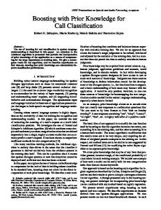
Update fk+1 = fk + Step 4 (Iteration): Increase k by one and repeat Step 2 and Step 3 if k < k∗ . Although this original boosting algorithm was proved to be consistent [3] and overfitting resistant [17], a series of studies [9], [24], [29] showed that its numerical convergence rate is far slower than that of the best nonlinear approximant. The main reason is that the linear search in Algorithm 1 makes fk be not always the greediest one. In particular, as shown in Fig.1, if fk−1 walks along the direction of gk to θ0 gk , then there usually exists a weak learner g such that the angle α = β . That is, after θ0 gk , continuing to walk along gk is no more the greediest one. However, the linear search makes fk−1 go along the direction of gk to θ1 gk .
Q(f ) = ED φ(f (X), Y ),
J
and Qm (f ) = EZ φ(f (X), Y ) =
m 1 X φ(f (Xi ), Yi ), m i=1
where ED is the expectation over the unknown true joint distribution D of (X, Y ) and EZ is the empirical expectation based on the sample Zm . Let S = {g1 , . . . , gn } be the set of weak learners (classifiers or regressors) and define Span(S) =
n X
j=1
J
aj gj : gj ∈ S, aj ∈ R, n ∈ N .
We assume that φ, therefore Qm , is Fr´echet differentiable and denote by Q′m (f, h) = (∇Qm (f ), h) the value of
rk-1 α β O Fig. 1.
θ0 J k
θ1Jk Jk
The drawback of boosting
Under this circumstance, an advisable method is to control the step-size in the linear search step of Algorithm 1. Thus, various variants of boosting, comprising the RTboosting, RSboosting and ε-boosting, have been
3
developed based on different strategies to control the step-size. It is obvious that the main difficulty of these schemes roots in how to select an appropriate step-size. If the step size is too large, then these algorithms may face the same problem as that of Algorithm 1. On the other hand, if the step size is too small, then the numerical convergence rate is also fairly slow [8]. Different from the aforementioned strategies that focus on controlling the step-size of gk∗ , we drive a novel direction to improve the numerical convergence rate and consequently, the generalization capability of boosting. The core idea is that if the approximation (or learning) effect of the k-th iteration is not good, then we regard fk to be too aggressive and therefore shrink it within a certain extent. That is, if a new iteration is employed, then we impose a re-scale operator on the estimator fk . This is the reason why we call our new strategy as the re-scale boosting (RBoosting). The following Algorithm 2 depicts the main idea of RBoosting. Algorithm 2 Re-scale boosting Step 1 (Initialization): Given data {(Xi , Yi ) : i = 1, . . . , m}, weak learner set S , a set of shrinkage de∗ gree {αk }∞ k=1 , iteration number k , and f0 ∈ Span(S). Step 2 (Projection of gradient): Find gk∗ ∈ S such that −Q′m (fk−1 , gk∗ )
=
sup −Q′m (fk−1 , g). g∈S
Step 3 (Linear search): Find βk∗ ∈ R such that
Qm ((1−αk )fk +βk∗ gk∗ ) = inf Qm ((1−αk )fk +βk gk∗ ) βk ∈R
Update fk+1 = (1 − αk )fk + βk∗ gk∗ . Step 4 (Iteration): Increase k by one and repeat Step 2 and Step 3 if k < k∗ . Compared Algorithm 2 with Algorithm 1, the only difference is that we employ a re-scale operator (1 − αk )fk in the linear search step of RBoosting. Here and hereafter, we call αk as the shrinkage degree. It can be easily found that RBoosting is similar as the greedy algorithm with free relaxation (GAFR) [30] and the X greedy algorithm with relaxation (XGAR)1 [28], [33] in sparse approximation. In fact, RBoosting can be regarded as a marriage of GAFR and XGAR. To be detailed, we adopt the projection of gradient of GAFR and the linear search of XGAR to develop Algorithm 2. 1
In [33], XGAR was called as the sequential greedy algorithm, while in [2], XGAR was named as the relaxed greedy algorithm for brevity.
It should be also pointed out that the present paper is not the first one to apply relaxed greedy-type algorithms in the realm of boosting. In particular, for the L2 loss, XGAR has already been utilized to design a boostingtype algorithm for regression in [1]. Since in both GAFR and XGAR, one needs to tune two parameters simultaneously in an optimization problem, GAFR and XGAR are time-consuming when faced with a general convex loss function. This problem is successfully avoided in RBoosting. III. T HEORETICAL
BEHAVIORS OF
RB OOSTING
In this section, we study the theoretical behaviors of RBoosting. We hope to address three basic issues regarding RBoosting, including its numerical convergence rate, consistency and generalization error estimate. To state the main results, some assumptions concerning the loss function φ and dictionary S should be presented. The first one is a boundedness assumption of S . Assumption 1: For arbitrary g ∈ S and x ∈ X , there exists a constant C1 such that n X i=1
gi2 (x) ≤ C1 .
Assumption 1 is certainly a bit stricter than the assumption supg∈S,x∈X |gi (x)| ≤ 1 in [30], [34]. Introducing such a condition is only for the purpose of deriving a fast numerical convergence rate of RBoosting with general convex loss functions. In fact, for a concrete loss function such as the Lp loss with 1 ≤ p ≤ ∞, Assumption 1 can be relaxed to supg∈S,x∈X |gi (x)| ≤ 1 [28]. Assumption 1 essentially depicts the localization properties of the weak learners. Indeed, it states that, for arbitrary fixed x ∈ X , expert for a small number of weak learners, all the |gi (x)|′ s are very small. Thus, it holds for almost all the widely used weak learns such as the trees [18], stumps [34], neural networks [1] and splines [7]. Moreover, for arbitrary dictionary ′ S ′ = {g1′ , . . . , gq n }, we can rebuild it as S = {g1 , . . . , gn } Pn ′ 2 with gi = gi′ /( i=1 (gi ) (x)). It should be noted that Assumption 1 is the only condition concerning the dictionary throughout the paper, which is different from [3], [34] that additionally imposed either VC-dimension or Rademacher complexity constraints to the weak learner set S . We then give some restrictions to the loss function, which have already adopted in [3], [4], [33], [34]. Assumption 2: (i) If |f (x)| ≤ R1 , |y| ≤ R2 , then there exists a continuous function Hφ such that |φ(f, y)| ≤ Hφ (R1 , R2 ).
(1)
4
(ii) Let D = {f : Qm (f ) ≤ Qm (0)} and f ∗ = minf ∈D Qm (f ). Assume that ∀c1 , c2 satisfying Qm (f ∗ ) ≤ c1 < c2 ≤ Qm (0), there holds 0
′′
≤ inf{Qm (f, g) : c1 < Q(f ) < c2 , g ∈ S} (2) ′′
≤ sup{Qm (f, g) : Qm (f ) < c2 , h ∈ S} < ∞. (3)
It should be pointed out that (i) concerns the boundedness of φ and therefore is mild. In fact, if R1 and R2 are bounded, then (i) implies that φ(f, y) is also bounded. It is obvious that (i) holds for almost all commonly used loss functions. Once φ is given, Hφ (R1 , R2 ) can be determined directly. For example, if φ is the L2 loss for regression, then Hφ (R1 , R2 ) ≤ (R1 + R2 )2 ; if φ is the exponential loss for classification, then R2 = 1 and Hφ (R1 , R2 ) ≤ exp{R1 }; if φ is the logistic loss for classification, then Hφ (R1 , R2 ) ≤ log(1 + exp{R1 }). P As Qm (f ) = m i=1 φ(f (Xi ), Yi ), conditions (2) and (3) actually describe the strict convexity and smoothness of φ as well as Qm . Condition (2) guarantees the strict convexity of Qm in a certain direction. Under this condition, the maximization (and minimization) in projection of gradient step (and linear search step) of Algorithms 1 and 2 are well defined. Condition (3) determines the smoothness property of Qm (f ). For arbitrary f (x) ∈ [−λ, λ], define the first and second moduli of smoothness of Qm (f ) as ρ1 (Qm , u) = sup |Qm (f + uh) − Qm (f )|, f,khk=1
and ρ2 (Qm , u) =
sup |Qm (f + uh)
f,khk=1
+ Qm (f − uh) − 2Qm (f )|,
where k·k denotes the uniform norm. It is easy to deduce that if (3) holds, then there exist constants C2 and C3 depending only on λ and c2 such that ρ1 (Qm , u) ≤ C2 kuk, and ρ2 (Qm , u) ≤ C3 kuk2 . (4)
It is easy to verify that all the widely used loss functions such as the L2 loss, exponential loss and logistic loss satisfy Assumption 2. By the help of the above stations, we are in a position to present the first theorem, which focuses on the numerical convergence rate of RBoosting. Theorem 1: Let fk be the estimator defined by Algo3 rithm 2. If Assumptions 1 and 2 hold and αk = k+3 , then for any h ∈ Span(S), there holds Qm (fk ) − Qm (h) ≤ C(khk21 + log k)k−1 ,
(5)
where C is a constant depending only on c1 , c2 , C1 , and khk1 =
inf n
(aj )j=1 ∈Rn
n X
j=1
|aj |, for h =
n X
aj gj .
j=1
If φ(f, y) = (f (x) − y)2 and S is an orthogonal basis, then there exists an h∗ ∈ Span(S) with bounded kh∗ k1 such that [9] |Qm (fk ) − Qm (h∗ )| ≥ Ck−1 ,
where C is an absolute constant. Therefore, the numerical convergence rate deduced in (5) is almost optimal in the sense that for at least some loss functions (such as the L2 loss) and certain dictionaries (such as the orthogonal basis), up to a logarithmic factor, the deduced rate is optimal. Compared with the relaxed greedy algorithm for convex optimization [10], [30] that achieves the optimal numerical convergence rate, the rate derived in (5) seems a bit slower. However, in [10], [30], the set D = {f : Qm (f ) ≤ Qm (0)} is assumed to be bounded. This is a quite strict assumption and, to the best of our knowledge, it is difficult to verify whether the widely used L2 loss, exponential loss and logistic loss satisfy this condition. In Theorem 1, we omit this condition in the cost of adding an additional logarithmic factor to the numerical convergence rate and some other easy-checked assumptions to the loss function and dictionary. Finally, we give an explanation why we select the 3 shrinkage degree αk as αk = k+3 . From the definition of fk , it follows that the numerical convergence rate may depend on the shrinkage degree. In particular, Bagirov et al. [1], Barron et al. [2] and Temlyakov [28] used different αk to derive the optimal numerical convergence rates of relaxed-type greedy algorithms. After checking our proof, we find that our result remains correct for C4 arbitrary αk = C5 k+C < 1 with C4 , C5 , C6 some finite 6 positive integers. The only difference is that the constant C in (5) may be different for different αk . We select 3 is only for the sake of brevity. αk = k+3 Now we turn to derive both the consistency and learning rate of RBoosting. The consistency of the boosting-type algorithms describes whether the risk of boosting can approximate the Bayes risk within arbitrary accuracy when m is large enough, while the learning rate depicts its convergence rate. Several authors have shown that Algorithm 1 with some specific loss functions is consistent. Three most important results can be found in [3], [4], [22]. Jiang [22] proved a process consistency property for Algorithm 1, under certain assumptions. Process consistency means that there exists a sequence {tm } such that if boosting with sample size m is stopped after tm iterations, its risk approaches the Bayes
5
risk. However, Jiang imposed strong conditions on the underlying distribution: the distribution of X has to be absolutely continuous with respect to the Lebesgue measure. Furthermore, the result derived in [22] didn’t give any hint on when the algorithm should be stopped since the proof was not constructive. [3], [4] improved the result of [22] and demonstrated that a simple stopping rule is sufficient for consistency: the number of iterations is a fixed function of m. However, it can also be found in [3], [4] that the deduced learning rate was fairly slow. [3, Th.6] showed that the risk of boosting converges to the Bayes risk within a logarithmic speed. Without loss of generality, we assume |Yi | ≤ M almost surely with M > 0. The following Theorem 2 plays a crucial role in deducing both the consistency and fast learning rate of RBoosting. Theorem 2: Let fk be the estimator obtained in Al3 gorithm 2. If αk = k+3 and Assumptions 1 and 2 hold, then for arbitrary h ∈ Span(S), there holds E{Q(fk ) − Q(h)} ≤
C(khk21
−1
+ log k)k k(log m + log k) , +C ′ (Hφ (log k, M ) + Hφ (khk1 , M )) m
where C and C ′ are constants depending only on c1 , c2 and C1 . Before giving the consistency of RBoosting, we should give some explanations and remarks to Theorem 2. Firstly, we present the values of Hφ (log k, M ) and Hφ (khk1 , M ). Taking Hφ (log k, M ) for example, if φ is the L2 loss for regression, then Hφ (log k, M ) = (log k+ M )2 , if φ is the logistic loss for classification, then Hφ (log k, M ) = log(k + 1) and if φ is the exponential loss for classification, then Hφ (log k, M ) = k. Secondly, we provide a simple method to improve the bound in Theorem 2. Let πM f (x) := min{M, |f (x)|}sgn(f (x)) be the truncation operator at level M . As Y ∈ [−M, M ] almost surely, there holds [36] E{Q(πM fk ) − Q(h)} ≤ E{Q(fk ) − Q(h)}.
Noting that there is not any computation to do such a truncation, this truncation technique has been widely used to rebuild the estimator and improve the learning rate of boosting [1]–[4]. However, this approach has a drawback: the usage of the truncation operator entails that the estimator πM fk is (in general) not an element of Span(S). That is, one aims to build an estimator in a class and actually obtains an estimator out of it. This is the reason why we do not introduce the truncation operator in Theorem 2. Indeed, if we use the truncation operator, then the same method as that in the proof of Theorem 2 leads to the following Corollary 1.
Corollary 1: Let fk be the estimator obtained in Al3 gorithm 2. If αk = k+3 and Assumptions 1 and 2 hold, then for arbitrary h ∈ Span(S), there holds E{Q(πM fk ) − Q(h)} ≤ C(khk21 + log k)k−1 k(log m + log k) , +C ′ (Hφ (M, M ) + Hφ (khk1 , M )) m
where C and C ′ are constants depending only on c1 , c2 and C1 . By the help of Theorem 2, we can derive the consistency of RBoosting. Corollary 2: Let fk be the estimator obtained in Al3 gorithm 2. If αk = k+3 , Assumptions 1 and 2 hold and k → ∞,
Hφ (log k, M )k log m → 0, when m → ∞, m (6)
then E{Q(fk )} →
inf
f ∈Span(S)
Q(f ), when m → ∞.
Corollary 2 shows that if the number of iterations satisfies (6), then RBoosting is consistent. We should point out that if the loss function is specified, then, we can deduce a concrete relation between k and m to yield the consistency. For example, if φ is the logistic function, then the condition (6) becomes k ∼ mγ with 0 < γ < 1. This condition is somewhat looser than the previous studies concerning the consistency of boosting [3], [4], [22] or its modified version [2], [34]. When used to both classification and regression, there usually is an overfitting resistance phenomenon of boosting as well as its modified versions [7], [34]. Our result shown in Corollary 2 looks to contradict it at the first glance, as k must be smaller than m. We illustrate that this is not the case. It can be found in [7], [34] that expect for Assumption 1, there is another condition such as the covering number, VC-dimension, or Rademacher complexity imposed to the dictionary. We highlight that if the dictionary of RBoosting is endowed with a similar assumption, then the condition k < m can be omitted by using the similar methods in [4], [23], [34]. In short, our assertions show that whether RBoosting is overfiiting resistant depends on the dictionary. At last, we give a learning rate analysis of RBoosting, which is also a consequence of Theorem 2. Corollary 3: Let fk be the estimator obtained in Al3 gorithm 2. Suppose that αk = k+3 and Assumptions 1 and 2 hold. For arbitrary h ∈ Span(S), if k satisfies k∼
s
m , Hφ (log k, M ) + Hφ (khk1 , M )
(7)
6
A. Toy simulations
then there holds E{Q(fk ) − Q(h)}
(8)
q
≤ C ′ ( Hφ (log m, M ) + Hφ (khk1 , M )
+khk21 )m−1/2 log m, C′
where C and are constants depending only on c1 , c2 and C1 and M . The learning rate (8) together with the stopping criteria (7) depends heavily on φ. If φ is the logistic loss for classification, then Hφ (log m, M ) = log(m + 1) and Hφ (khk1 , M ) = log(khk1 + 1), we thus derive from (8) that, E{Q(fk )−Q(h)} ≤ C ′ (log(m+1)+khk21 )m−1/2 log m.
We encourage the readers to compare our result with [34, Th.3.2]. Without the Rademacher assumptions, RBoosting theoretically performs at least the same as that of RTboosting. If φ is the L2 loss for regression, we can deduce that ′
E{Q(fk ) − Q(h)} ≤ C (log m +
khk21 )m−1/2 log m,
which is almost the same as the result in [1]. If φ is the exponential loss for classification, by setting k ∼ m1/3 , we can derive E{Q(fk ) − Q(h)} ≤ C ′ (log m + ekhk1 )m−1/3 log m,
which is much faster than AdaBoost [3]. It should be noted that if the truncation operator is imposed to the RBoosting estimator, then the learning rate of the rescale AdaBoost can also be improved to E{Q(πM fk ) − Q(h)} ≤ C ′ (log m + ekhk1 )m−1/2 log m.
IV. N UMERICAL R ESULTS In this section, we conduct a series of toy simulations and real data experiments to demonstrate the promising outperformance of the proposed RBoosting over the original boosting algorithm. For comparison, three other popular boosting-type algorithms, i.e., ǫ-boosting [20], RSboosting [18] and RTboosting [34], are also considered. In the following experiments, we utilize the L2 loss function for regression (namely, L2Boost) and logistic loss function for classification (namely, LogitBoost). Furthermore, we use the CART [6] (with the number of splits J = 4) to build up the week learners for regression tasks in the toy simulations and decision stumps (with the number of splits J = 1) to build up the week learners for regression tasks in real data experiments and all classification tasks.
We first consider numerical simulations for regression problems.The data are drawn from the following model: Y = m(X) + σ · ε,
(9)
where X is uniformly distributed on [−2, 2]d with d ∈ {1, 10}, ε, independent of X , is the standard gaussian noise and the noise level σ varies among in {0, 0.3, 0.6, 1}. Two typical regression functions [1] are considered in the simulations. One is a univariate piecewise function defined by ( √ 10 −x sin(8πx), ≤ x < 0, m1 (x) = (10) 0, else, and the other is a multivariate continuously differentiable sine function defined as m2 (x) =
10 X
(−1)j−1 xj sin(xj 2 ).
(11)
j=1
For these regression functions and all values of σ , we generate a training set of size 500, and then collect an independent validation data set of size 500 to select the parameters of each boosting algorithms: the number of iterations k, the regularization parameter ν of RSboosting, the truncation value of RTboosting, the shrinkage degree of RBoosting and ε of ε-boosting. In all the numerical examples, we chose ν and ǫ from a 20 points set whose elements are uniformly localized in [0.01, 1]. We select the truncated value of RTboosting the same as that in [34]. To tune the shrinkage degree, αk = 2/(k + u), we employ 20 values of u which are drawn logarithmic equally spaced between 1 to 106 . To compare the performances of all the mentioned methods, a test set of 1000 noiseless observations is used to evaluate the performance in terms of the root mean squared error (RMSE). Table I documents the mean RMSE over 50 independent runs. The standard errors are also reported (numbers in parentheses). Several observations can be easily drawn from Table I. Firstly, concerning the generalization capability, all the variants essentially outperform the original boosting algorithm. This is not a surprising result since all the variants introduce an additional parameter. Secondly, RBoosting performs as the almost optimal variant since its RMSEs are the smallest or almost smallest for all the simulations. This means that, if we only focus on the generalization capability, then RBoosting is a preferable choice. In the second toy simulation, we consider the “orange data” model which was used in [37] for binary classification. We generate 100 data points for each class to build
7
TABLE I P ERFORMANCE COMPARISON OF DIFFERENT BOOSTING ALGORITHMS ON σ
Boosting
0 0.3 0.6 1
0.2698(0.0495) 0.6204(0.0851) 0.7339(0.0706) 1.1823(0.0483)
0 0.3 0.6 1
2.3393(0.1112) 2.4051(0.1112) 2.4350(0.0836) 2.6583(0.1103)
SIMULATED REGRESSION DATA EXAMPLES
RSboosting RTboosting RBoosting piecewise function (10) 0.2517(0.0561) 0.3107(0.0905) 0.2460(0.0605) 0.4635(0.0728) 0.5131(0.0735) 0.5112(0.0779) 0.7317(0.0392) 0.7475(0.0333) 0.7206(0.0486) 1.1474(0.0485) 1.1776(0.0604) 1.1489(0.0485) continuously differentiable sine functions (11) 1.7460(0.0973) 1.8388(0.1102) 1.6166(0.0955) 1.7970(0.0951) 1.8380(0.0830) 1.6732(0.0928) 1.8866(0.0837) 1.9628(0.0853) 1.7730(0.0832) 2.0671(0.0789) 2.1575(0.0891) 1.9870(0.1092)
up the training set. Both classes have two independent standard normal inputs x1 , x2 , but the inputs for the second class conditioned on 4.5 ≤ x21 + x22 ≤ 8. Similarly, to make the classification more difficult, independent feature noise q were added to the inputs. One can find more details about this data set in [37]. Table II reports the classification accuracy of five boosting-type algorithms over 50 independent runs. Numbers in parentheses are the standard errors. In this simulation, for q varies among {0, 2, 4, 6}, we generate a validation set of size 200 for tuning the parameters, and then 4000 observations to evaluate the performances in terms of classification error. For this classification task, RBoosting outperforms the original boosting in terms of the generalization error. It can also be found that as far as the classification problem is concerned, RBoosting is at least comparable to other variants. Here we do not compare the performance with the performance of SVMs reported in [37], because the main purpose of our simulation is to highlight the outperformance of the proposed RBoosting over the original boosting. All the above toy simulations from regression to classification verify the theoretical assertions in the last section and illustrate the merits of RBoosting. B. Real Data Examples In this subsection, We pursue the performance of RBoosting on eight real data sets (the first five data sets for regression and the others for classification). The first data set is the Diabetes data set [13]. This data set contains 442 diabetes patients that are measured on ten independent variables, i.e., age, sex, body mass index etc. and one response variable, i.e., a measure of disease progression. The second one is the Boston Housing data set created from a housing values survey in suburbs of Boston by Harrison and Rubinfeld [21]. This data set contains 506 instances which include thirteen attributions, i.e., per capita crime rate by town,
ǫ-boosting 0.2306(0.0827) 0.4844(0.0862) 0.7403(0.0766) 1.1395( 0.0590) 1.7434(0.0804) 1.7665(0.0718) 1.8895(0.0880) 2.0766(0.0956)
proportion of non-retail business acres per town, average number of rooms per dwelling etc. and one response variable, i.e., median value of owner-occupied homes. The third one is the Concrete Compressive Strength (CCS) data set created from [32]. The data set contains 1030 instances including eight quantitative independent variables, i.e., age and ingredients etc. and one dependent variable, i.e., quantitative concrete compressive strength. The fourth one is the Prostate cancer data set derived from a study of prostate cancer by Blake et al. [5]. The data set consists of the medical records of 97 patients who were about to receive a radical prostatectomy. The predictors are eight clinical measures, i.e., cancer volume, prostate weight, age etc. and one response variable, i.e., the logarithm of prostate-specific antigen. The fifth one is the Abalone data set, which comes from an original study in [25] for predicting the age of abalone from physical measurements. The data set contains 4177 instances which were measured on eight independent variables, i.e., length, sex, height etc. and one response variable, i.e., the number of rings. For classification task, three benchmark data sets are considered, namely Spam, Ionosphere and WDBC, which can be obtained from UCI Machine Learning Repository. Spam data contains 4601 instances, and 57 attributes. These data are used to measure whether an instance is considered to be spam. WDBC (Wisconsin Diagnostic Breast Cancer) data contains 569 instances, and 30 features. These data are used to identify whether an instance is diagnosed to be malignant or benign. Ionosphere data contains 351 instances, and 34 attributes. These data are used to measure whether an instance was “good” or “bad”. For each real data, we randomly (according to the uniform distribution) select 50% data for training, 25% data to build the validation set for tuning the parameters and the remainder 25% data as the test set for evaluating the performances of different boosting-type algorithms. We repeat such randomization 20 times and report the average errors and standard errors (numbers
8
TABLE II P ERFORMANCE COMPARISON OF DIFFERENT BOOSTING ALGORITHMS ON q 0 2 4 6
Boosting 11.19(1.32)% 11.27(1.29)% 11.79(1.54)% 12.02(1.62)%
RSboosting 10.36(1.16)% 10.48(1.24)% 10.79(1.21)% 10.93(1.21)%
RTboosting 10.50(1.19)% 10.71(1.19)% 11.07(1.41)% 11.20(1.23)%
SIMULATED “ ORANGE DATA ” EXAMPLE
RBoosting 10.44(1.12)% 10.59(1.25)% 10.90(1.24)% 10.91(1.28)%
ǫ-boosting 10.29(1.17)% 10.60(1.28)% 10.94(1.26)% 11.02(1.32)%
TABLE III P ERFORMANCE COMPARISON OF DIFFERENT BOOSTING ALGORITHMS ON REAL DATA EXAMPLES dataset Diabetes Housing CCS Prostate Abalone Spam Ionosphere WDBC
Boosting 59.0371(4.1959) 4.4126(0.5311) 5.4345(0.5473) 0.3131(0.0598) 2.2180(0.0710) 6.06(0.60)% 8.27(2.88)% 5.31(2.11)%
RSboosting 55.3109(3.6591) 4.2742(0.7026) 5.2049(0.1678) 0.1544(0.0672) 2.1934(0.0504) 5.13(0.52)% 5.80(1.92)% 2.45(1.39)%
in parentheses) in Table III. The parameter selection strategies of all boosting-type algorithms are the same as those in the toy simulations. It can be easily observed that, all the variants outperform the original boosting algorithm to a large extent. Furthermore, RBoosting at least performs as the second best algorithm among all the variants. Thus, the results of real data coincide with the toy simulations and therefore, experimentally verify our theoretical assertions. That is, all the experimental results show that the new idea “re-scale” of RBoosting is numerically efficient and comparable to the idea “regularization” of other variants of boosting. This paves a new road to improve the performance of boosting. V. P ROOF
OF
T HEOREM 1
RTboosting 56.1343(3.2543) 4.3685(0.3929) 5.5826(0.1901) 0.2450(0.0631) 2.3633(0.0762) 5.24(0.48)% 6.09(2.24)% 2.69(1.58)%
RBoosting 55.6552(4.5351) 4.1752(0.3406) 5.3711(0.1807) 0.1193(0.0360) 2.1922(0.0574) 5.06(0.55)% 5.23(2.31)% 2.09(1.55)%
ǫ-boosting 57.7947(3.3970) 4.1244(0.3322) 5.9621(0.1960) 0.1939(0.0545) 2.2098(0.0474) 5.02(0.51)% 5.92(2.64)% 2.52(1.33)%
then av+1 ≤ av (1 − c2 /v).
Then, for all n = 1, 2, . . . , we have c2 +c
1+ c1 −c1
an ≤ 2
2
1
C0 n−c1 .
Proof: For 1 ≤ v ≤ j0 , the inequality av ≥ C0 v −c1
implies that the set V = {v : av ≥ C0 v −c1 }
does not contain v = 1, 2, . . . , j0 . We now prove that for any segment [n, n + k] ⊂ V , there holds c1 +1
To prove Theorem 1, we need the following three lemmas. The first one is a small generalization of [28, Lemma 2.3]. For the sake of completeness, we give a simple proof. Lemma 1: Let j0 > 2 be a natural number. Suppose that three positive numbers c1 < c2 ≤ j0 , C0 be given. Assume that a sequence {an }∞ n=1 has the following two properties: (i) For all 1 ≤ n ≤ j0 , an ≤ C 0 n
−c1
,
and, for all n ≥ j0 , an ≤ an−1 + C0 (n − 1)−c1 .
(ii) If for some v ≥ j0 we have av ≥ C0 v −c1 ,
k ≤ (2 c2 −c1 − 1)n.
Indeed, let n ≥ j0 + 1 be such that n − 1 ∈ / V , which means an+j ≥ C0 (n + j)−c1 , j = 0, 1, . . . , k.
Then by the conditions (i) and (ii), we get an+k ≤ an Πn+k−1 v=n (1 − c2 /v)
≤ (an−1 + C0 (n − 1)−c1 )Πn+k−1 n=n (1 − c2 /v).
Thus, we have (n + k)−c1 ≤
an+k ≤ 2(n − 1)−c1 Πn+k−1 v=n (1 − c2 /v), C0
where c2 ≤ j0 ≤ v . Taking logarithms and using the inequalities ln(1 − t) ≤ −t, t ∈ [0, 1);
9 m−1 X v=n
v −1 ≥
Z
m
t−1 dt = ln(m/n),
n
we can derive that n+k−1 X n+k −c1 ln ≤ ln 2 + ln(1 − c2 /v) n−1 v=n
≤ ln 2 −
Hence,
n+k−1 X v=n
n+k c2 /v ≤ ln 2 − c2 ln . n
(c2 − c1 ) ln(n + k) ≤ ln 2 + (c2 − c1 ) ln n + c1 ln
which implies
n , n−1
where M1 (S) = {span(S) : kf k1 ≤ 1}. Proof of Theorem 1: We divide the proof into two steps. The first step is to deduce an upper bound of fk in the uniform metric. Since fk+1 = (1 − αk+1 )fk + ∗ g ∗ , we have βk+1 k+1 fk = fk+1 +
Noting Qm (f ) is twice differential, if we use the Taylor expansion around fk+1 , then Qm (fk ) = Qm (fk+1 ) +
(c1 +1)/(c2 −c1 )
n+k ≤2
and
�
k≤ 2
n +
c1 +1 c2 −c1
�
− 1 n.
=
Let us take any m ∈ N. If m ∈ / V , we have the desired inequality. Assume m ∈ V and let [n, n + k] be the maximal segment in V containing m, then we obtain
− +
am ≤ an ≤ an−1 + C0 (n − 1)−c1 ≤ 2C0 (n − 1)−c1 � �−c1 −c1 n − 1 ≤ 2C0 m . m �
c1 +1
�
Since k ≤ 2 c2 −c1 − 1 n, we then have 2
c +c1 1 m n+k ≤ ≤ 2 c2 −c1 . n−1 n This means that
am ≤ 2C0 m−c1 2
c2 +c1 1 c2 −c1
Qm (g) ≥ Qm (f ) + Q′m (f, g − f ),
or, in other words, Qm (f ) − Qm (g) ≤ Q′m (f, f − g) = −Q′m (f, g − f ).
Based on this, we can obtain the following lemma, which was proved in [30, Lemma 1.1]. Lemma 2: Let Qm be a Fr´echet differential convex function. Then the following inequality holds for f ∈ D 0 ≤ Qm (f
+ ug) − Qm (f ) − uQ′m(f, g)
≤ 2ρ(A, ukgk).
To aid the proof, we also need the following lemma, which can be found in [27, Lemma 2.2]. Lemma 3: For any bounded linear F and any dictionary S , we have sup F (g) = g∈S
sup f ∈M1 (S)
+
F (f ),
∗ g∗ αk+1 fk+1 − βk+1 k+1 fk+1 , 1 − αk+1 � � ∗ ∗ ∗ gk+1 1 ′′ ˆ αk+1 fk+1 − βk+1 Qm f k , 2 1 − αk+1 αk+1 Qm (fk+1 ) + Q′ (fk+1 , fk+1 ) 1 − αk+1 m ∗ βk+1 ∗ � Q′m fk+1 , gk+1 1 − αk+1 � � α2k+1 ′′ Qm fˆk , fk+1 2 2(1 − αk+1 ) ∗ )2 � � (βk+1 ′′ ˆk , gk+1 , Q f 2(1 − αk+1 )2 m
Q′m
�
�
where ∗
∗
αk+1 fk+1 − βk+1 gk+1 + θfk+1 fˆ = (1 − θ) 1 − αk+1
for some θ ∈ (0, 1). For the convexity of Qm , we have � � α2k+1 ′′ ˆk , fk+1 ≥ 0. Q f 2(1 − αk+1 )2 m
,
which finishes the proof of Lemma 1. The convexity of Qm implies that for any f, g,
∗ g∗ αk+1 fk+1 − βk+1 k+1 . 1 − αk+1
Furthermore, if we use the fact that fk+1 is the minimum ∗ , then it is easy on the path from (1−αk+1 )fk along gk+1 to see that ∗ � Q′m fk+1 , gk+1 = 0.
According to the convexity of Qm again, we obtain Q′m (fk+1 , fk+1 ) ≥ Qm (fk+1 ) − Qm (0).
Noting that
αk+1 1−αk+1
= k4 , we obtain
4 Qm (fk ) ≥ Qm (fk+1 ) + (Qm (fk+1 ) − Qm (0)) k ∗ )2 � � (βk+1 ′′ Qm fˆk , gk+1 . + 2
If we write B = inf{Q′′m (f, g) : c1 < Qm (f ) < c2 , g ∈ S}, then we have ∗ (βj+1 )2
4 2 Qm (fj ) − Qm (fj+1 ) + Qm (0) . ≤ B j �
�
10
Therefore,
Therefore,
k X
2 log k (βj∗ )2 ≤ . B j=0
Qm (fk+1 ) − Qm (h) ≤ Qm (fk ) − Qm (h)
−αk+1 (Qm (fk ) − Qm (h))
Then it follows from the definition of fk that
�
+2ρ Qm , (khk1 +
fk = (1 − αk )(1 − αk−1 ) · · · (1 − α2 )β1∗ g1∗ + (1 − αk )(1 − αk−1 ) · · · (1 − α3 )β2∗ g2∗
∗ ∗ + . . . + (1 − αk )βk−1 gk−1 + βk∗ gk∗ .
Therefore, it follows from the Assumption 1 that v u n k q uX X u |fk (x)| ≤ t (βj∗ )2 |gj∗ (x)|2 ≤ 2C1 log k/B. j=0
j=0
(12) Now we turn to the second step, which derives the numerical convergence rate of RBoosting. For arbitrary βk ∈ R and gk ∈ S , it follows form Lemma 2 that Qm ((1 − αk+1 )fk + βk+1 gk+1 )
≤ Qm (fk ) − βk+1 (−Q′m (fk , gk+1 ))
satisfies
Set βk = khk1 αk . It follows from Lemma 3 that g∈S
≥
−Q′m (fk , φ)
Qm (fk ) − Qm (h) ≤ C(khk21 + log k)k−1 ,
Under this circumstance, we get ∗ Qm ((1 − αk+1 )fk + βk+1 gk+1 )
where C is a constant depending only on B , C1 and C2 . This finishes the proof of Theorem 1.
≤ Qm (fk ) − αk+1 (−Q′m (fk , h − fk ))
∗ + 2ρ(Qm , kβk+1 gk+1 − αk+1 fk k).
VI. P ROOF
Based on Lemma 2, we obtain
Thus, ∗ Qm (fk+1 ) = Qm ((1 − αk+1 )fk + βk+1 gk+1 )
≤ Qm (fk ) − αk (Qm (fk ) − Q − m(h))
∗ + 2ρ(Qm , khk1 αk+1 gk+1 − αk+1 fk ).
khk1 αk+1 g ∗
k+1
− αk+1 fk
≤ khk1 αk+1 + αk+1 kfk k
≤ khk1 αk+1 + αk+1 kfk k1 ≤ (khk1 +
p
2C1 ln k)αk+1 .
OF
T HEOREM 2
To aid the proof of Theorem 2, we need the following two technical lemmas, both of them can be found in [36]. Let R > 0, we denote BR as the closed ball of Vk =Span{g1∗ , . . . , gk∗ } with radius R centered at origin:
−Q′m (fk , h − fk ) ≥ Qm (fk ) − Qm (h).
Furthermore, according to (12), we obtain
A(0) 9C2 + khk21 ≤ C0 , a2 ≤ C0 2−1 , 4 8 and for v ≥ 2, there holds a1 ≤
Thus the condition (ii) of Lemma 1 holds with c2 = 23 . Applying Lemma 1 we obtain
φ∈M1 (S) ′ −khk−1 1 Qm (fk , h).
Then, it follows from (13) and ρ(Qm , u) ≤ C2 u2 that
p
g∈S
sup
A(0) 72C2 288C1 C2 log k + khk21 + . 2 25 25B 2
+2C2 (khk1 + 2C1 log k/B)2 α2v+1 /av ) � � 3 1 ≤ av 1 − + v +�3 2v + 2 � 3 . ≤ av 1 − 2v
= sup −Q′m (fk , g).
sup −Q′m (fk , g) =
C0 = 2 +
av+1 ≤ av (1 − αv+1
+ 2ρ(Qm , kβk+1 gk+1 − αk+1 fk k).
∗ ) −Q′m (fk , gk+1
Now, we use the above inequality and Lemma 1 to prove Theorem 1. Let ak = Qm (fk+1)−Qm (h). Let c3 ∈ (1, 2] and C0 be selected later. We then prove the conditions (i) and (ii) of Lemma 1 hold for an appropriately selected C0 . Set
Thus the condition (i) of Lemma 1 holds with j0 = 2. and av ≥ C0 v −1 , then by (13), we get for v ≥ 6,
− αk+1 Q′m (fk , fk )
From Step 2 in Algorithm 2,
2C1 log k/B)αk+1 . (13)
av ≤ av−1 + C0 (v − 1)−1 .
= Qm (fk − αk+1 fk + βk+1 gk+1 )
∗ gk+1
�
p
BR = {f ∈ Vk : kf k ≤ R}.
Lemma 4: For R > 0 and η > 0, we have log N (BR , η) ≤ C3 k log
�
4R , η �
where N (BR , η) denotes the covering number of BR with radius η under the uniform norm. The following ratio probability inequality is a standard result in learning theory (see [36]).
11
Lemma 5: Let G be a set of functions on Z such that, for some c ≥ 0, |g − E(g)| ≤ B almost everywhere and E(g2 ) ≤ cE(g) for each g ∈ G . Then, for every ε > 0, there holds m 1 √ E(g) − m i=1 g(zi ) p P sup ≥ ε E(g) + ε f ∈G
(
)
P
(
mε ≤ N (G, ε) exp − 2c + 2B 3
)
.
Proof of Theorem 2: At first, we use the concentration inequality in Lemma 5 to bound Q(fk ) − Q(h) − (Qm (fk ) − Qm (h)).
We need apply Lemma 5 to the set of functions FR , where
It follows from (12) that fk ∈ BR with R = C5 log k, then with confidence at least � � � �� � C6 log k 3mε 1 − exp C3 k log , exp − ε 8C1 there holds Q(fk ) − Q(h) − (Qm (fk ) − Qm (h)) √ q ≤ ε( Q(fk ) − Q(h) + ε) 1 ≤ (Q(fk ) − Q(h)) + ε, 2 where C1 = C(h, C5 log k, M ). Therefore, with the same confidence, there holds Q(fk ) − Q(h) ≤ 2(Qm (fk ) − Qm (h)) + 2ε.
FR := {ψ(Z) = φ(f (X), Y ) − φ(h(X), Y ) : f ∈ BR } .
Since Assumptions 1 and 2 hold, it follows from Theorem 1 that for any function h ∈ Span(S), there holds
Using the obvious inequalities kf k∞ ≤ R, |y| ≤ M and khk∞ ≤ khk1 , from Assumption 1 it follows the inequalities
where C is a constant depending only on c1 , c2 and C1 . Combining the last two inequalities yields that
|ψ(Z)| ≤ Hφ (R, M ) + Hφ (khk1 , M )
T ≤ε
Qm (fk ) − Qm (h) ≤ C(khk21 + log k)k−1 ,
holds with at least
and
C6 log k 1 − exp C3 k log ε � � 3mε , × exp − 8C(h, C5 log k, M ) �
Eψ 2 ≤ (Hφ (R, M ) + Hφ (khk1 , M ))Eψ.
For ψ1 , ψ2 ∈ FR , it follows from Assumption 2 that there exists a constant C4 such that |ψ1 (Z) − ψ2 (Z)| = |φ(f1 , Y ) − φ(f2 , Y )| ≤ C4 |f1 (X) − f2 (X)|.
We then get
where Q(fk ) − Q(h) − C(khk21 + log k)k−1 . 2 For arbitrary µ > 0, there holds T =
N (FR , ε) ≤ N (BR , ε/C4 ).
Eρm (T ) =
According to Lemma 4, there holds log N (FR , ε) ≤ C3 k log
�
4C4 R . ε �
Employing Lemma 5 with B = c = Hφ (R, M ) + Hφ (khk1 , M ) and Eψ = Q(f ) − Q(h),
m 1 X ψ(Zi ) = Qm (f ) − Qm (h), m i=1
we have, for every ε > 0, Q(f ) − Q(h) − (Qm (f ) − Qm (h)) √ p ≤ ε sup Q(f ) − Q(h) + ε f ∈BR
with confidence at least �� � � � � 3mε 4C4 R exp − , 1 − exp C3 k log ε 8C(h, R, M ) where C(h, R, M ) = (Hφ (R, M ) + Hφ (khk1 , M )).
��
�
∞
Z
∞
P{T > ε}dε
0�
C6 log k 3mε ≤ µ+ exp C3 k log − dε ε 8C1 µ �Z ∞� � � C6 log k C3 k 3mµ dε ≤ µ + exp − 8C1 ε µ �� � � C6 log k C3 k 3mµ µ. ≤ µ + exp − 8C1 µ Z
By setting µ = yields
C1 C3 k(log m+log k) , 3m
E(T ) ≤
�
direct computation
2C1 C3 k(log m + log k) . 3m
That is, E{Q(fk ) − Q(h)}
4C1 C3 k(log m + log k) , 3m which finishes the proof Theorem 2. ≤ C(khk21 + log k)k−1 +
12
VII. C ONCLUSION
AND FURTHER DISCUSSIONS
In this paper, we proposed a new idea to conquer the slow numerical convergence rate problem of boosting and then develop a new variant of boosting, named as the re-scale boosting (RBoosting). Different from other variants such as the ε-boosting, RTboosting, RSboosting that control the step-size in the linear search step, RBoosting focuses on alternating the direction of linear search via implementing a re-scale operator on the composite estimator obtained by the previous iteration step. Both theoretical and experimental studies illustrated that RBoosting outperformed the original boosting and performed at least comparable to other variants of boosting. Theoretically, we proved that the numerical convergence rate of RBoosting was almost optimal in the sense that it cannot be essentially improved. Using this property, we then deduced a fairly tight generalization error bound of RBoosting, which was a new “record” for boosting-type algorithms. Experimentally, we showed that for a number of numerical experiments, RBoosting outperformed boosting, and performed at least the second best of all variants of boosting. All these results implied that RBoosting was an reasonable improvement of Boosting and the idea “re-scale” provided a new direction to improve the performance of boosting. To stimulate more opinions from others on RBoosting, we present the following two remarks at the end of this paper. Remark 1: Throughout the paper, up to the theoretical optimality, we can not provide any essential advantages of RBoosting in applications, which makes it difficult to persuade the readers to use RBoosting rather than other variants of boosting. We highlight that there may be two merits of RBoosting in applications. The first one is that, due to the good theoretical behavior, if the parameters of RBoosting are appropriately selected, then RBoosting may outperform other variants. This conclusion was partly verified in our experimental studies in the sense that for all the numerical examples, RBoosting performed at least the second best. The other merit is that, compared with other variants, RBoosting cheers a totally different direction to improve the performance of boosting. Therefore, it paves a new way to understand and improve boosting. Furthermore, we guess that if the idea of the “re-scale” in RBoosting and “regularization” in other variants of boosting are synthesized to develop a new boosting-type algorithm, such as the re-scale εboosting, re-scale RTboosting, then the performance may be further improved. We will keep working on this issue and report our progress in a future publication. Remark 2: According to the “no free lunch” philos-
ophy, all the variants improve the learning performance of boosting at the cost of introducing additional parameters, such as the truncated parameter in RTboosting, regularization parameter in RSboosting, ε in ε-Boosting, and shrinkage degree in RBoosting. To facilitate the use of these variants, one should also present strategies to select such parameters. In particular, Elith et al. [14] showed that 0.1 is a feasible choice of ε in ε-Boosting; B¨uhlmann and Hothorn [8] recommended the selection of 0.1 for the regularization parameter in RSboosting; Zhang and Yu [34] proved that O(k−2/3 ) is a good value of the truncated parameter in RTboosting. One may naturally ask: how to select the shrinkage degree αk in RBoosting? This is a good question and we find a bit headache to answer it. Admittedly, in this paper, we do not give any essential suggestion to practically attack this question. In fact, αk plays an important role in RBoosting. If αk is too small, then RBoosting performs similar as the original boosting, which can be regarded as a special RBoosting with αk = 0. If αk is too large, an extreme case is αk close to 1, then the numerical convergence rate of RBoosting is also slow. Although we theoretically present some values of the αk , the best one in applications, we think, should be selected via some model selection strategies. We leave this important issue into a future study [31], where the concrete role of the shrinkage degree will be revealed. ACKNOWLEDGEMENT The research was supported by the National Natural Science Foundation of China (Grant No. 11401462) and the National 973 Programming (2013CB329404). R EFERENCES [1] A. Bagirov, C. Clausen, and M. Kohler. An L2 boosting algorithm for estimation of a regression function. IEEE. Trans. Inform. Theory, 56: 1417-1429, 2010. [2] A. Barron, A. Cohen, W. Dahmen, and R. DeVore. Approximation and learning by greedy algorithms. Ann. Statist., 36: 64-94. 2008. [3] P. Bartlett, and M. Traskin. AdaBoost is consistent. J. Mach. Learn. Res., 8: 2347-2368, 2007. [4] P. Bickel, Y. Ritov, and A. Zakai. Some theory for generalized boosting algorithms. 7: 705-732, 2006. [5] C. Blake and C. Merz. {UCI} repository of machine learning databases, 1998. [6] L. Breiman, J. Friedman, C. Stone, and R. Olshen. Classification and Regression Trees. CRC press, 1984. [7] P. Buhlmann, and B. Yu. Boosting with the L2 loss: regression and classification. J. Amer. Statist. Assoc., 98: 324-339, 2003. [8] P. Buhlmann, and T. Hothorn. Boosting algorithms: regularization, prediction and model fitting. Statist. Sci., 22: 477-505, 2007. [9] R. DeVore, and V. Temlyakov. Some remarks on greedy algorithms. Adv. Comput. Math., 5: 173-187, 1996.
13
[10] R. DeVore, and V. Temlyakov. Convex optimization on Banach spaces. arXiv:1401.0334v1, 2014. [11] N. Duffy, and D. Helmbold. Boosting methods for regression. Mach. Learn., 47: 153-200, 2002. [12] J. Ehrlinger, and H. Ishwaran. Characterizing L2 boosting. Ann. Statist. 40: 1074-1101, 2012. [13] B. Efron, T. Hastie, I. Johnstone, and R. Tibsirani. Least angle regressionn. Ann. Statist., 32: 407-451, 2004. [14] J. Elith, J. R. Leathwick, and T. Hastie. A working guide to boosted regression trees. Journal of Animal Ecology. 77: 802813, 2008. [15] Y. Freund. Boosting a weak learning algorithm by majority. Inform. & Comput., 121: 256-285, 1995. [16] Y. Freund, and R. Schapire. Experiments with a new boosting algorithm. In Machine Learning: Proc. Thirteenth Intern. Conf., pages 148-156. Morgan Kauffman, 1996. [17] J. Friedman, T. Hastie, and R. Tibshirani. Additive logistic regression: a statistical view of boosting (With discussion and a rejoinder by the authors). Ann. Statist., 28: 337-407, 2000. [18] J. Friedman. Greedy function approximation: a gradient boosting machine. Ann. Statist., 29: 1189-1232, 2001. [19] L. Gy¨orfy, M. Kohler, A. Krzyzak and H. Walk. A Distribution-Free Theory of Nonparametric Regression. Springer, Berlin, 2002. [20] T. Hastie, J. Taylor, R. Tibshirani, and G. Walther. Forward stagewise regression and the monotone lasso. Elec. J. Statist., 1: 1-29, 2007. [21] D. Harrison and D. L. Rubinfeld. Hedonic prices and the demand for clean air. J. Environ. Econ., 5(1):81–102, 1978. [22] W. Jiang. Process consistency for adaboost. Ann. Statist., 32: 13-29, 2004. [23] S. Lin, Y. Rong, X. Sun, and Z. Xu. Learning capability of relaxed greedy algorithms. IEEE Trans. Neural Netw. & Learn. Syst., 24: 1598-1608, 2013. [24] E. Livshits. Lower bounds for the rate of convergence of greedy algorithms. Izvestiya: Mathematics 73: 1197-1215, 2009. [25] W. Nash, T. Sellers, S. Talbot, A. Cawthorn, and W. Ford. The population biology of abalone (haliotis species) in tasmania. i. blacklip abalone (h. rubra) from the north coast and islands of bass strait. Sea Fisheries Division, Technical Report, no. 48, 1994. [26] R. Schapire. The strength of weak learnability. Mach. Learn., 5: 1997-2027, 1990. [27] V. Temlyakov. Greedy algorithms in Banach spaces. Adv. Comput. Math., 14: 277-292, 2001. [28] V. Temlyakov. Relaxation in greedy approximation. Constr. Approx., 28: 1-25, 2008. [29] V. Temlyakov. Greedy approximation. Acta Numer., 17: 235409, 2008. [30] V. Temlyakov. Greedy approximation in convex optimization. arXiv: 1206.0392v1, 2012. [31] L.Xu, S. B. Lin, Y. Wang, and Z. B. Xu. Shrinkage degree in L2 -re-scale boosting for regression. Submitted to IEEE Trans. Neural Netw. & Learn. Syst., 2015. [32] I. C. Ye. Modeling of strength of high performance concrete using artificial neural networks. Cement and Concrete Research, 28(12): 1797-1808, 1998. [33] T. Zhang. Sequential greedy approximation for certain convex optimization problems. IEEE Trans. Inform. Theory, 49: 682691, 2013. [34] T. Zhang, and B. Yu. Boosting with early stopping: convergence and consistency. Ann. Statis., 33: 1538-1579, 2005. [35] P. Zhao, and B. Yu. Stagewise lasso. J. Mach. Learn. Res., 8: 2701-2726, 2007.
[36] D. Zhou, and K. Jetter. Approximation with polynomial kernels and SVM classifiers. Adv. Comput. Math., 25: 323-344, 2006. [37] J. Zhu, S. Rosset, T. Hastie, and R. Tibshirani. 1-norm support vector machines. Neural Information Proceeding Systems 16, 2003.