The Constructive Method for Query Containment ... - Semantic Scholar

The Constructive Method for Query Containment Checking (extended version)

Carles Farré, Ernest Teniente, Toni Urpí Universitat Politècnica de Catalunya E-08034 Barcelona -- Catalonia [farre | teniente | urpi]@lsi.upc.es

Abstract. We present a new method that checks Query Containment for queries with negated derived atoms and/or integrity constraints. Existing methods for Query Containment checking that deal with these cases do not check actually containment but another related property called uniform containment, which is a sufficient but not necessary condition for containment. Our method can be seen as an extension of the canonical databases approach beyond the class of conjunctive queries.

1

Introduction

Query Containment (QC) [Ull89] is the problem concerned with checking whether the answers that a query obtains on a database are a subset of the answers obtained by another query on the same database, for every possible content of the database. QC is applied in several contexts: query optimization by removing redundant subexpressions [Ull89], materialized view and cache reuse [LMSS95], integrity constraint redundancy checking [GSUW94], etc. An important amount of research has been devoted to QC checking over the last 20 years [CM77, ASU79, JK83, Klu88, Sag88, Ull89, CV92, LMSS93, LS93, ZO93, LS95, DS96, ST96, CR97]. However, most of this research focused on obtaining optimal algorithms for conjunctive queries, i.e. those queries defined by just one deductive rule containing only positive base atoms. There are frequent situations where negated atoms can help to improve the expressive power of deductive rules [Ull88]. In this paper, we present a new method that checks Query Containment for queries with safe stratified negation on derived (view) predicates. Previous methods that deal with safe stratified negation can be classified into two different approaches. The first approach is taken by those methods that check QC for a restricted class of queries with negation. In [LS95, Ull94] negation was considered only on base atoms. Instead, Levy et al. [LMSS93] dealt with save stratified negation on derived predicates but requiring every base predicate to be 1-ary. The second approach is represented by those methods in [LS93, ST96]

1

that do not check actually QC but another related property called Uniform Containment [Sag88], which is a sufficient but not necessary condition for QC. The following example illustrates the limitations of these methods. Consider, for instance, a deductive database consisting of two base predicates. Emp(x) indicates that x is an employee. Works_for(x, y) indicates that x works for y. There are also two derived predicates: Boss(x), when x has someone else working for him/her; and Chief(x) when x has some boss working for him/her. Boss(x) ← Works_for(z, x) Chief(x) ← Works_for(y, x) ∧ Boss(y) Then we define two queries with the same predicate query, Sub(x) -x is a subordinate-: Q1: Sub(x) ← Emp(x) ∧ ¬Chief(x). Q 2: Sub(x) ← Emp(x) ∧ ¬Boss(x) Intuitively, Q1 retrieves employees that are not Chief, that is, those employees that do not have any boss working for them. Instead, Q2 retrieves employees that are not bosses, that is, those employees that have nobody working for them. In this sense, Q1 is less restrictive than Q2 because Q2 does not allow anyone to work for x, while Q1 only applies this restriction to the ones that are Boss. Hence, we can find a database, like {Emp(joan), Works_for(ann, joan)}, showing that the answers that Q 1 obtains, i.e. Sub(joan), are not always answers to Q 2. Therefore, Q1 is not contained in Q 2. We will see how our method reaches the same conclusion in section 3.1 of the paper. Conversely, if Q1 is less restrictive than Q2 then all the answers to Q2 will be also answers to Q1. Therefore, Q2 is contained in Q1. However, this simple example cannot be handled in a satisfactory way by the methods proposed in the literature. Clearly, this example does not fall into the classes of queries covered in [LMSS93, LS95, Ull94]. On the other hand, the methods of [LS93, ST96] would prove that Q1 is not uniform contained in Q2 and Q2 is not uniform contained in Q1 (see section 7.2 below), but these results does not help to determine whether Q1 – Q2 or Q2 – Q1 hold. When considering the integrity constraints defined in a database, the containment relationship between two queries does not need to hold for any state of the database but only for those that satisfy the integrity constraints. This idea is captured by the notion of IC-compliant Query Containment. Again, current methods that handle IC-compliant QC [Sag88, ST96, DS96] take the uniform containment approach. Our method checks both "true" IC-compliant QC and QC in a uniform and integrated way. Roughly, the main idea of our Constructive Method for Query Containment Checking is to construct a counterexample that proves the [IC-compliant] QC relationship that we want to check. The facts added to this counterexample are instantiated according to the same patterns that are applied when constructing the set of canonical databases used for conjunctive query containment checking [Klu88, Ull89, LS93, Ull94]. If this constructive procedure fails, then [IC-compliant] QC holds. The Constructive Method for Query Containment Checking is based on the reduction of the QC problem to the view-updating problem [FTU98]. In particular, our method specializes the Events Method for view updating [TO95] to focus more on the characteristic aspects of QC checking. Our 2

approach is similar to that of [LMSS93, LS95], which translates QC to the problem of query satisfiability. However, the query-satisfiability methods that [LMSS93, LS95] provide impose stronger restrictions on the cases that they handle, and they do not consider IC-compliant QC. This paper is organized as follows. Section 2 reviews basic concepts needed in the rest of the paper. Section 3 presents the Constructive Method for [IC-compliant] Query Containment Checking with safe stratified negated negation. Section 4 introduces the formalization of the method. In section 5, we prove correctness and completeness of our method. Section 6 discusses some decidability issues. Section 7 reviews the related work. Finally, we present conclusions and points out further work in section 8.

2

Base Concepts

In this section, we briefly review some definitions related to Deductive Databases, Queries and QC [Llo87, Ull88, Sag88]. A deductive database D is a triple D = (EDB, DR, IC) where EDB is a finite set of facts, DR a finite set of deductive rules, and IC a finite set of integrity constraints. A deductive rule is a formula of the form: P(t1, …, tn) ← L1 ∧ … ∧ Lm with n ≥ 0, m ≥ 1. P(t1, …, tn) is called the head and L1 ∧ … ∧ Lm is the body. Variables are assumed to be universally quantified over the whole formula. Predicates in the body may be ordinary, base and derived predicates, or evaluable ("built-in"), e.g. arithmetic comparisons. Base predicates appear only in EDB and (eventually) in the body of deductive rules. Derived (view) predicates appear only in DR. Evaluable predicates can be evaluated without accessing the database. As usual, we require safeness, that is, the variables appearing in negated atoms and evaluable ones, must also appear in an ordinary positive literal in the same rule body; and stratified negation, that is, there must not be negative literals about recursively defined derived predicates. In this way, the evaluation of the deductive rules on EDB is done stratum by stratum and its result, DR(EDB), is the perfect model of DR and EDB. An integrity constraint is a formula that every EDB is required to satisfy. We deal with constraints in denial form1: ← L1 ∧ … ∧ Lm with m ≥ 1. For the sake of uniformity, we associate to each integrity constraint an inconsistency predicate Icn. Then, we would rewrite the former denial as an integrity rule Ic1 ← L1 ∧ … ∧ Lm. We also define an standard auxiliary predicate Ic with the following rules: Ic ← Ic1, …, Ic ← Icn, one for each integrity constraint of the database. A fact Ic will indicate that there is an integrity constraint that is violated. A query Q for a deductive database D is a finite set of deductive rules that defines a dedicated nary query predicate Q. Without loss of generality, we assume that all predicates other than Q appearing in Q belong to D.

1

More general constraints can be transformed into this form by applying the procedure described in [LT84]

3

The answer to the query is the set of all ground facts about Q obtained as a result of evaluating the deductive rules from both Q and DR on EDB: {Q(a i1,..., ain) | Q(a i1 ,..., ain) ∈ (Q∪DR)(EDB)} Therefore, a query Q1 is contained in an another query Q2 when the set of ground facts answering Q1 is a subset of the set of ground facts answering Q2, regardless of the underlying EDB. Definition 2.1. Let Q 1 and Q2 be two queries defining the same n-ary query predicate Q on a deductive database D = (EDB, DR, IC). Q1 is contained in Q2 , written Q 1 – Q2 , if {Q(a i1 ,..., a in) | Q(ai1,..., ain) ∈ (Q1∪DR)(EDB)} ∑ {Q(a k1,...,akn) | Q(a k1,...,akn) ∈ (Q2∪DR)(EDB)} for any EDB. When considering integrity constraints, the containment relationship between two queries must not hold for any EDB but only for consistent EDB’s, i.e. those that satisfy the integrity constraints. As stated before, we assume that the database contains an inconsistency predicate Ic that holds whenever some integrity constraint is violated. Thus, consistent EDB’s are those where the fact Ic does not hold. Definition 2.2. Let Q 1 and Q2 be two queries defining the same n-ary query predicate Q on a deductive database D = (EDB, DR, IC). Q1 is IC-compliant contained in Q2 , written Q 1 –IC Q2 , if {Q(a i1,..., ain) | Q(a i1 ,..., ain) ∈ (Q1∪DR)(EDB)} ∑ {Q(a k1,...,akn) | Q(a k1,...,akn) ∈ (Q2∪DR)(EDB)} for any EDB such that Ic „ (IC∪DR)(EDB).

3

The Constructive Query Containment Method

As we have just seen, the containment relationship between two queries must hold for the whole set of possible databases in the general case, or for those that satisfy the integrity constraints in the IC-compliant case. A suitable way of checking QC is to check the lack of containment, that is, to find just one EDB where the containment relationship that we want to check does not hold: Definition 3.1. Q 1 is not contained in Q 2, written Q 1 « Q 2, if there is an EDB such that {Q(a i1,..., ain) | Q(a i1 ,..., ain) ∈ (Q1∪DR)(EDB)} ⊄ {Q(a k1,...,akn) | Q(a k1,...,akn) ∈ (Q2∪DR)(EDB)} Definition 3.2. Q 1 is not IC-compliant contained in Q 2, written Q 1 «IC Q 2, if there is a consistent EDB, i.e. Ic „ (IC∪DR)(EDB), such that {Q(a i1,..., ain) | Q(a i1 ,..., ain) ∈ (Q 1∪DR)(EDB)} ⊄ {Q(ak1,...,akn) | Q(ak1,...,akn) ∈ (Q 2∪DR)(EDB)} Given Q1 and Q2 two queries defining the same n-ary query predicate Q on a deductive database D = (EDB, DR, IC), our Constructive Query Containment Method, CQC method for shorthand, is addressed to construct one EDB T where the presumed containment relationship does not hold. If the method succeeds, noncontainment is proved. Otherwise, i.e. no EDB may be built, it means that the containment relationship holds. Before using the CQC method, we must define a noncontainment goal expressing the noncontainment relationship between two queries, Q1 and Q2, to be satisfied by the resulting EDB T. We define the noncontainment goal NC = ← Q 1 (x 1 ,...,x n ) ∧ ¬Q 2 (x 1 ,...,x n ) when we want to prove that Q1 – Q2 does not hold. That is, NC holds on an EDB where a fact about Q1 is true but Q2 is false for the same values. We define NC = ← Q1(x1,...,xn) ∧ ¬Q2(x1,...,xn) ∧ ¬Ic when we want to prove that Q1 –IC Q2 is false. In this case, we ensure that the target EDB does not violate 4

any integrity constraint by requiring ¬Ic be true in the goal. Notice that we need to rename the query predicates Q, by adding a suffix to their names, to identify properly their respective defining rule(s). Positive literals in the noncontainment goal NC define information that must be present in the target EDB to prove the desired goal NC. Since a query predicate like Q1 is always defined in terms of other predicates, we must unfold it until we reach a goal where positive predicates are all base. Those base predicates determine the information to be included in the EDB T. Moreover, the goal resulting from unfolding NC will always contain negative literals. ¬Q2(x1,...,xn), for instance, will always be one of such literals but other negative literals may also appear during the unfolding process. Negative literals correspond to conditions that must be enforced to guarantee that the noncontainment goal NC remains satisfied. For instance, in the particular case of ¬Q 2 (x 1 ,...,x n ), we have to guarantee that base facts required for making Q 1 (x 1 ,...,x n ) true do not make also Q 2 (x 1 ,...,x n ) true at the same time. When one of such conditions is violated, we have to look for additional facts to be included in T to make it succeed again. Therefore, we can see the work performed by the CQC method for satisfying the noncontainment goal as an interleaving of two activities: 1) including base facts in the ongoing target EDB T (constructive derivation); and 2) enforcing that negative literals found during 1) are not satisfied by the current T (consistency derivation). For the sake of generality, the CQC method performs those activities along the way depending on whether the considered literal is positive or negative, instead of unfolding first and enforcing consistency afterwards. In the remaining of the section we illustrate how the Constructive Query Containment checking method works by applying it to the example presented in the paper introduction (section 3.1). Moreover, in section 3.2, we discuss the approach that our method takes to instantiate the facts to be inserted in the target EDB to refute the containment relationship. This approach has been inspired by the use of Canonical Databases to check QC for the class of conjunctive queries [Klu88, Ull89, LS93, Ull94]. In Appendix B, we show the execution outputs of an implementation of the CQQ method obtained from the following and other examples. An example of IC-complian QC cheching is also included.

3 . 1 Example Let us review the example we presented in the introduction, where we had a database D = (EDB, DR, IC) where EDB is a set of ground facts about two base predicates Emp(x) and Works_for(x, y), DR = { Boss(x) ← Works_for(z, x) Chief(x) ← Works_for(y, x) ∧ Boss(y) } and IC = Ø, that is, there is no integrity constraint.

5

We defined two queries with the same predicate query: Q1: Sub(x) ← Emp(x) ∧ ¬Chief(x) Q 2: Sub(x) ← Emp(x) ∧ ¬Boss(x).

Constructive CQC Derivation

Consistency CQC Derivation

← Sub1(x) ∧ ¬Sub2(x) A1

1

← Emp(x) ∧ ¬Chief(x) ∧ ¬Sub2(x) A3

2

← Chief(0)

T = {Emp(0)}

3.1

← ¬Chief(0) ∧ ¬Sub2(0)

← Works_for(y,0) ∧ Boss(y) C = {← Works_for(y,0) ∧ Boss(y) }

3

A4

4

4.1

4.3.2a z= 0 fails

B1

← Emp(0) ∧ ¬Boss(0)

4.3.1

4.2

← Works_for(z,0) A3

B3

← Sub2(0) ← Boss(0)

A1

3 .2 fails

← ¬Sub2(0) A4

B1

4.3.2b z= 1 [] T = {Emp(0), Works_for(1,0)}

B2

← ¬Boss(0) 4.3

B4

fails

[] T = {Emp(0), Works_for(1,0)}

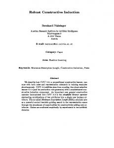
Fig. 3.1.

As we saw in the introduction, Q1 is less restrictive than Q 2, so we can conclude that Q1 is not contained in Q2. Now, let the CQC method prove that Q 1 – Q2 does not hold by constructing an EDB T satisfying the noncontainment goal NC = ← Sub1(x) ∧ ¬Sub 2(x) . Such a T is built by performing a constructive derivation for NC with R as initial input set, where R = {Sub1(x) ← Emp(x) ∧ ¬Chief(x) Sub2(x) ← Emp(x) ∧ ¬Boss(x) Boss(x) ← Works_for(z, x) Chief(x) ← Works_for(y, x) ∧ Boss(y)} is the set of deductive rules to consider.

6

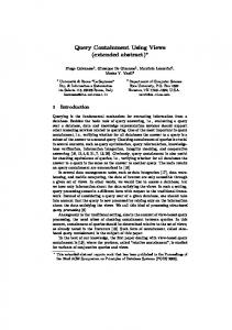
This constructive derivation is partially shown in figure 3.1. (circled labels appearing at each derivation step are references to the rules of the method, defined in section 4). For the sake of simplicity, we suppose left-to-right selection of literals. Note that T is empty initially. The first step is a SLDNF resolution step that uses R as input set to unfold the selected positive derived literal Sub1(x). At the second step, the selected literal is Emp(x), which is a positive base literal. To get a successful derivation, the method should instantiate x with a constant and include the new ground base fact in the input set and use it as input clause. The procedure assigns an arbitrary constant to x, say 0 for instance. Therefore Emp(0) is added to T. At step 3, the selected literal is ¬Chief(0). To get success for this constructive derivation, Chief(0) must not be true by T. This is guaranteed by enforcing a consistency derivation for {← Chief(0)} to fail using R∪(T={Emp(0)}) as input set. This consistency derivation is shown in the shaded right half of figure 3.1. Step 3.1 in this consistency derivation is a SLDNF resolution step that uses R as input set to unfold the selected derived atom Chief(0). Step 3.2 is a SLDNF resolution step that uses the current content of T as input set. Since Works_for(y, 0) cannot be unified with T={Emp(0)}, the consistency derivation fails. However, we must take into account that facts satisfying ← Works_for(y, 0) ∧ Boss(y) could be added to T in later constructive steps. To prevent this, our method uses an auxiliary set C, called condition set, to record those goals that fail with respect to the current T but could succeed afterwards. In this way, before including a new base fact in T the method will have to check that such an inclusion does not satisfy any condition of C. For this reason, the condition ← Works_for(y, 0) ∧ Boss(y) must be added to C. Since the consistency derivation for {← Chief(0)} fails, ¬Chief(0) is true at step 3 in the main constructive derivation. At step 4, the selected literal is ¬Sub 2(0). Hence, the CQC method calls a consistency derivation for {← Sub2(0)} with R∪(T={Emp(0)}), to guarantee that Sub2(0) is not satisfied by T. Step 4.1 in this second consistency derivation unfolds the selected literal Sub 2(0). Step 4.2 is a SLDNF resolution step where the selected literal, the positive base atom Emp(0), is unified with the current content of T. At step 4.3, the selected literal is ¬Boss(0). To ensure failure of this consistency derivation, Boss(0) must be made true. This is accomplished by performing a constructive derivation for ← Boss(0) with R∪(T={Emp(0)}). This subsidiary constructive derivation is shown enclosed in the light box on the left half of the figure 3.1 Step 4.3.1 in the subsidiary constructive derivation unfolds the selected literal Boss(0) as at step 1. At step 4.3.2a the selected literal is Works_for(z, 0). As at step 2, the method should instantiate z with a constant, e.g. the previously introduced constant 0, and include the new ground base fact in T. However, before adding Works_for(0, 0) to T, the CQC method must enforce that this insertion does not violate any condition of C. This is done by calling a consistency derivation for {← Works_for(y,0) ∧ Boss(y)} with R∪(T={Emp(0), Works_for(0,0)}). The fact is that such a new consistency derivation cannot be failed as it is shown in figure 3.2a. That is, the insertion of Works_for(0, 0) would violate the condition ← Works_for(y,0) ∧ Boss(y) and, thus, would make ¬Chief(0) false. After this failed attempt of making Works_for(z, 0) true, the method considers a new constant value, e.g. 1, at step 4.3.2b. Therefore, the current goal is to add Works_for(1,0) to T. Again, we must enforce that such a insertion does not violate any condition of C by calling a consistency derivation for {← Works_for(y,0) ∧ Boss(y)} with R∪(T={Emp(0), Works_for(1,0)}) This is done in steps 4.3.2b.1 to 4.3.2b.3 in figure 3.2b. In this case, the consistency derivation fails and then the method can include Works_for(1,0) in T. Note that, at step 4.3.2b.3, a new condition {← 7

Works_for(z,1)} has been added to C to enforce that 1 will not become a Boss. After performing step 4.3.2b, the subsidiary constructive derivation gets the empty clause and, so, it ends successfully. Therefore Boss(0) becomes true and the consistency derivation for {← Sub2(0)} fails at step 4.3.

Consistency CQC Derivation

Consistency CQC Derivation

← Works_for(y,0) ∧ Boss(y) 4.3.2a.1 ← Boss(0) 4.3.2a.2

← Works_for(y,0) ∧ Boss(y)

B2

4.3.2b.1 ← Boss(1)

B2

B1

4.3.2b.2 ← Works_for(z,1)

B1

← Works_for(z,0) 4.3.2a.3

C = {..., , ←Works_for(z,1)}

B2

[]

4.3.2b.3

B3

fails

Fig. 3.2a.

Fig. 3.2b

Returning to the main constructive derivation, these latter subsidiary derivations have allowed the method to make ¬Sub 2(0) true at step 4. After this successful step, no more literals remain to be made true and, thus, the CQC method gets the empty clause in the main constructive derivation. Hence, the constructive derivation for NC = ← Sub1(x) ∧ ¬Sub 2(x) is over successfully. The constructed EDB T is {Emp(0), Works_for(1,0)}, proving that Q1 « Q2. 3 . 2 Variable Instantiation Patterns Let us review now how the simulated execution of the CQC method has assigned constant values to the variables of the base facts added to T in the previous example. The following rules have been applied to instantiate variables: 1

For the sake of simplicity, all the variables range over the same domain: the domain of the positive integers.

2

Assign the integer value 0 to the first variable to be instantiated.

3

When a new variable must be instantiated, either 3.1 assign an integer already used in a previous instantiation; or 3.2 assign a new integer n = m + 1, where m was the highest constant value used for instantiating variables in some previous step. We enforce that only one new value can be introduced for each distinct variable.

In this way, the variable instantiations that have been taken into account in example 3.1 are x = 0; and z = 0, in a first failed attempt, and z = 1, as a successful alternative. If this latter instantiation had also failed, the CQC would have considered no other possible variable instantiation and the main constructive derivation would have failed definitely. The reason is that, in this example, any 8

other constant assignation to x and y would be isomorphic with respect to one considered previously. That is, any other possible instantiation of the two variables would produce the same result as either {x = z = 0} or {x = 0, z = 1}. Therefore, the aim of the CQC method is just to check the variable instantiations that are relevant to the derivations that it performs, but without loss of completeness. That is, we must enforce that all the possible relevant alternatives have been checked before accepting the failure of a constructive derivation. This principle for instantiating the base facts that the CQC method adds to the target EDB T is connected to, indeed it is inspired by, the concept of canonical databases [Klu88, Ull89, LS93, Ull94]. This concept is based on the idea that it is not necessary to check the whole (infinite) set of possible EDBs to prove containment but only a (finite) subset of them, the set of canonical EDBs. In this way, if we prove that a containment relationship holds on any canonical EDB, then QC holds for any EDB. The soundness of this approach is guaranteed by proving that any possible EDB is represented by one canonical EDB and that this correspondence preserves the containment relationship. The canonical databases-based approach for QC checking can be applied suitably for the class of conjunctive queries, where queries are expressed in terms of base and/or evaluable atoms. In this case, the whole set of canonical databases is bounded a priori and it is generated easily before performing the containment tests. In contrast, the CQC method is intended to construct dynamically just one canonical EDB, the one that proves that QC does not hold, following a testand-error approach. In this way, the method fails to prove noncontainment after having discarded all the canonical databases as solutions. Since our method can deal with negated derived atoms and/or integrity constraints, we can see the CQC method as an extension the canonical databases-approach beyond the class of conjunctive queries. In the same way as the number and the kind of canonical databases to take into account depend on the concrete subclass of conjunctive queries that are considered, we distinguish two different variable instantiation patterns, VIPs for shorthand. Each one of them defines how the CQC method has to instantiate the base facts to be added to the target EDB T according to the queries and deductive rules that are examined. Negation VIP: It is applied when there is negation but not arithmetic comparisons. The variable instantiation procedure performed in the example 3.1 is a naive implementation of this VIP. The EDBs generated and tested with this VIP correspond to the canonical EDBs considered in [Ull94] for the conjunctive query case with negation. See section 7.1 for a more detailed comparison with [Ull94]. General VIP: It is applied when there are arithmetic comparisons, with or without negation. The EDBs generated and tested with this VIP correspond to the canonical EDBs considered in [Klu88] for the conjunctive query case. Each canonical EDBs, called representative in [Klu88], represents a different allowable arrangement of variable instantiations according to the total order relationship of the considered value domain. See Appendix B.3 for a concrete example. These different VIPs are described formally in section 4.

9

4

Formalization of The Constructive Query Containment Method

As shown in previous examples, our method is an interleaving of two activities: 1) including base facts in the ongoing target EDB T; and 2) enforcing that negative literals found during 1) are not made true by the current T. These two activities are performed during constructive and consistency derivations, respectively, as defined below. Let Q1 and Q2 be two queries defining the same n-ary query predicate Q on a deductive database D = (EDB, DR, IC). Let NC = ← Q 1(x1,...,xn) ∧ ¬Q 2(x1,...,xn) [∧ ¬Ic] be a noncontainment goal. If the CQC method performs a constructive derivation from (NC ∅ ∅ K) to ([] T C K’) with R = DR∪Q1∪Q2[∪IC] as initial input set, then Q 1 « Q 2. [] is the empty clause. T is an EDB that satisfies the noncontainment goal NC. K is the set of constant values appearing in R. K’ is the set of constant values appearing in R∪T. C is the condition set where the method has recorded those goals appeared during the derivation that T must not satisfy. If no such derivation exists, the noncontainment goal can not be satisfied and we conclude that Q 1 is contained in Q 2. In section 5 we prove the soundness and completeness of our method. For convenience, let from now on G\L stand for the goal obtained from a goal G by dropping a selected occurrence of literal L in G.

4 . 2 Constructive Derivation A constructive derivation from (G 1 T1 C 1 K 1) to (G n Tn C n Kn) via a safe computation rule P [Llo87] is a sequence (G1 T1 C1 K1), (G2 T2 C2 K2), …, (Gn Tn Cn Kn) such that for each i ≥ 1, Gi has the form ←L1 ∧…∧ Lk, P(Gi) = Lj and (Gi+1 Ti+1 Ci+1 Ki+1) is obtained according to one of the following rules: A1) If Lj is a positive derived atom, then Gi+1= S, where S is the resolvent of some clause in R with Gi on the selected literal Lj, Ti+1= Ti , Ci+1= Ci and Ki+1= Ki. A2) If Lj is a ground positive base atom and there exists a consistency derivation from (Ci Ti∪{Lj} Ci Ki) to ({} T’ C’ K’), then G i+1= Gi\Lj, Ti+1= T’, C i+1=C’ and Ki+1= K’. Note that if Ci = ∅ or Lj ∈ Ti then Gi+1 = ←L1 ∧…∧ Lj-1 ∧ Lj+1∧…∧ L k, Ti+1 = Ti∪{Lj}, C i+1= C i and Ki+1= Ki. A3) If Lj is a nonground positive base atom and x is the set of its nonground variables, then there is a CQC variable instantiation procedure from (x, ∅, Ki) to (∅, σ, Ks) leading to a variable substitution σ that assigns to each variable in x a constant from K s according to some variable instantiation pattern. Moreover, if there exists a consistency derivation from (Ci Ti∪{Ljσ} Ci Ks) to ({} T’ C’ K’), then G i+1= Gi\Lj, Ti+1= T’, C i+1=C’ and K i+1= K’. Note that if Ci = ∅ or Ljσ ∈ Ti then G i+1 = ←L1 ∧…∧ Lj-1 ∧ Lj+1∧…∧ L k, Ti+1 = Ti∪{Ljσ}, Ci+1= Ci and Ki+1= Ks. A4) If Lj is negative and there is a consistency derivation from ({←¬L j} Ti C i Ki) to ({} T’ C’ K’), then G i+1= G i\Lj, T i+1= T’, C i+1=C’ and K i+1=K’. A5) If Lj is an evaluable literal and it is evaluated true, then Gi+1= Gi\Lj, Ti+1= Ti, Ci+1= Ci and K i+1= K i.

10

Rule A1) is an SLDNF resolution step where R acts as input set. In rule A2), the selected base atom is included in the EDB T i, in order to get a successful derivation for the current branch, provided that the atom does not violate the condition set Ci. Rule A3) is similar to A2) but we first need to instantiate the base atom according to the appropriate variable instantiation pattern. In rule A4), we get the next goal if we can ensure consistency for the selected literal. In rule A5), we just evaluate the selected evaluable literal. Variable Instantiation Procedure. A variable instantiation procedure from (x 0 θ 0 K 0) to (x n θ n Kn) is a sequence (x0 θ0 K0), (x1 θ1 K1), …, (xn θn Kn) such that for each i ≥ 0, xi is a set of variables {xi1, …, xik}, θi is a substitution of variables per constants and Ki is a set of constants. (x i+1 θ i+1 Ki+1) is obtained according to one of the following variable instantiation patterns: Negation VIP. Apply one of the following two rules: NVIP_1)

xi+1 = xi\xi1, θi+1 = θ1∪{xi1/k} and Ki+1 = Ki, where k ∈ Ki;

NVIP_2)

xi+1 = xi\xi1, θi+1 = θ1∪{xi1/k} and Ki+1 = Ki∪{k}, where k ∉ Ki.

General VIP. Apply one of the following four rules: GVIP_1)

xi+1 = xi\xi1, σi+1 = σ1∪{xi1/k} and Ki+1 = Ki, where k ∈ Ki;

GVIP_2)

xi+1 = xi\xi1, σi+1 = σ1∪{xi1/k} and Ki+1 = Ki∪{k}, where k < min(Ki);

GVIP_3) xi+1 = xi\xi1, σi+1 = σ1∪{xi1/k} and Ki+1 = Ki∪{k}, where kj < k < k j+1, kj,kj+1 ∈ Ki and there is no kh ∈ Ki such that kj < kh < kj+1; GVIP_4)

xi+1 = xi\xi1, σi+1 = σ1∪{xi1/k} and Ki+1 = Ki∪{k}, where max(Ki) < k.

Additionally, the CQC variable instantiation procedure must enforce that if it instantiates a variable by applying one of the preceding rules that introduce new constants (NVIP_2, GVIP_2, GVIP_3 or GVIP_4), then such an instantiation cannot be reconsidered afterwards with other constant. The CQC method uses the Negation VIP when the are negation but not arithmetic comparisons in R. In this case, each distinct variable gets either a previous introduced constant or a new one. The General VIP is applied when there are arithmetic comparisons in R. In this case, each distinct variable gets a constant according to either an old or a new location in the total order of constants introduced previously.

4 . 2 Consistency Derivation A consistency derivation from (F1 T1 C1 K1) to (Fn Tn C n Kn) via a safe computation rule P is a sequence (F1 T1 C 1 K 1), (F 2 T2 C 2 K 2),…, (Fn Tn C n Kn) such that for each i ≥ 1, F i has the form {Hi} ∪ F’ i, where Hi = ← L1 ∧ … ∧ Lk and, for some j=1…k, (F i+1 Ti+1 C i+1 Ki+1) is obtained according to one of the following rules: B1) If Lj is a positive derived atom, S’ is the set of all resolvents of clauses in R with Hi on the selected literal Lj and [] ∉ S’, then F i+1= S’∪F’ i, Ti+1= T i, Ci+1= Ci and Ki+1= K i. Note that if no input clause in R can be unified with Lj, then S’ = ∅ and Fi+1= F’i.

11

B2) If Lj is a positive base atom, S’ is the set of all resolvents of clauses in Ti with Hi on the selected literal Lj and [] ∉ S’, then Fi+1= S’∪F’i, Ti+1= Ti, Ci+1=Ci∪ {Hi} and Ki+1= K i. If Lj is fully grounded then Ci+1=Ci. B3) If Lj is a positive base atom and no input clause in Ti can be unified with Lj, then F i+1= F’i and Ti+1 = Ti, Ci+1= Ci∪ {Hi} and Ki+1= Ki. B4) If Lj is a ground negative ordinary literal, k > 1 and there is a consistency derivation from ({←¬Lj} Ti C i Ki) to ({} T’ C’ K’), then F i+1= {H i\L j}∪F’i, T i+1=T’, Ci+1= C’ and K i+1= K’. B5) If Lj is a ground negative ordinary literal and there is a constructive derivation from (←¬L j T i C i Ki) to ([] T’ C’ K’), then F i+1=F’i, T i+1=T’, C i+1= C’ and K i+1= K’. B6) If Lj is a ground evaluable literal, it is evaluated true and k > 1 then F i+1= {H i\L j}∪F’i, Ti+1= Ti, C i+1= C i and Ki+1= Ki. B7) If Lj is a ground evaluable literal and it is evaluated false, then F i+1= F’ i, Ti+1= T i, C i+1= C i and Ki+1= Ki. Rules B1) and B2) are SLDNF resolution steps where either R or T acts as input set, respectively. In rule B3) the current branch is dropped from the consistency derivation because already determined T ensures failure for it. Moreover, the current goal Hi must be included in condition set Ci in order to guarantee that later additions to Ti will not make this branch succeed. In rules B5) and B4) the current branch will be dropped or not depending on whether there is a constructive or a consistency derivation for the negation of the selected literal. In rules B7) and B6) the current branch will be dropped or not depending on whether the selected literal is evaluated false or true. Consistency derivations do not rely on the particular order in which selection rule P selects literals since, in general, all possible ways in which a conjunction ← L1 ∧ … ∧ Lk can fail should be explored before concluding that it cannot be failed.

5

Soundness and Completeness Containment Method

of

the

Constructive

Query

In this section, we summarize the main results concerning the soundness and completeness results of the CQC method. The detailed proofs are given in Appendix A. Such proofs rely on the soundness and completeness of the SLNDF resolution. In this way, if the SLDNF resolution is sound and complete in the deductive framework that we consider, then the CQC method is also sound and complete. Let Q1 and Q2 be two queries defining the same n-ary query predicate Q on a deductive database D = (EDB, DR, IC) and NC = ← Q 1(x1,...,xn) ∧ ¬Q 2 (x 1 ,...,x n ) [∧ ¬Ic] the noncontainment goal. If the CQC method performs a constructive derivation from (NC ∅ ∅ K) to ([] T C K’) with R = DR∪Q1∪Q2[∪IC] as initial input set, then we prove that there exist an SLDNF refutation of R ∪ T ∪ {NC} (soundness). Conversely, if there exists an EDB Tx such there is an SLDNF refutation

12

of R ∪ Tx ∪ {NC}, then we prove that the CQC method performs a constructive derivation from (NC ∅ ∅ K) to ([] T C K’), where T ∑ Tx (completeness). 5 . 2 Soundness The CQC method is sound in the sense that if the method obtains an EDB T for a noncontainment goal NC, then the noncontainment relationship expressed by NC holds in T. Soundness of the CQC method is based on the following Lemma: Lemma 5.1: Let R be a set of deductive rules, K the set of constant values appearing in R, G a goal and T an EDB such that there exists a constructive derivation from (G ∅ ∅ K) to ([] T C K’). Then there exists a SLDNF refutation of R ∪ T ∪ {G}. As it can be seen, the lemma relates the constructive derivation from (G ∅ ∅ K) to ([] T C K’) of our method to an SLDNF refutation of R ∪ T ∪ {G}. Given that SLDNF resolution has been proved sound [Cla78], then the following theorem follows: Theorem 5.2: (Soundness of the CQC Method) Let Q1 and Q2 be two queries defining the same n-ary query predicate Q on a deductive database D = (EDB, DR, IC). If T is an EDB obtained by the CQC Method on the noncontainment goal NC = ← Q 1(x 1,...,x n) ∧ ¬Q 2(x 1,...,x n) [∧ ¬Ic], then Q 1 « Q 2 (Q1 « IC Q 2). Proof: From lemma 5.1, there exists an SLDNF refutation of R ∪ T ∪ {NC} if there exists a constructive derivation from (NC ∅ ∅ K) to ([] T C K’), where R = DR∪Q1∪Q2[∪IC] and K is the set of constants appearing in R. Then, by the soundness of the SLDNF resolution, it follows that ∃ x 1 ,...,x n ( Q 1 (x 1 ,...,x n ) ∧ ¬Q 2 (x 1 ,...,x n ) [∧ ¬Ic]) is a logical consequence of comp(R∪T) and, thus, Q 1 « Q 2 (Q1 « IC Q 2). ∆ 5 . 2 Completeness The CQC method is complete in the sense that if Q1 « Q2 (Q1 «IC Q2), then the method obtains an EDB T for the noncontainment goal NC = ← Q1(x1,...,xn) ∧ ¬Q2(x1,...,xn) [∧ ¬Ic]. Completeness of the CQC method is based on the following Theorem: Theorem 5.3: Let R be a set of deductive rules, K the set of constant values appearing in R, T and T’ EDBs and G a goal. If there exists a SLDNF refutation of R ∪ T’ ∪ {G} then there exists a constructive derivation from (G ∅ ∅ K) to ([] T C K’) where T ∑ T’. In this case, we relate the completeness of the CQC Method to that of the SLDNF resolution. [CL89] showed that SLDNF resolution is complete for databases and goals that are allowed, strict2 and stratified.

2

A set of deductive rules P is strict if there is no pair F, F’ of nodes in the dependency graph of P shuch that F depends evenly and oddly on F’. See [CL89] for more details.

13

Theorem 5.4: (Completeness of the CQC Method) Let Q1 and Q2 be two queries defining the same n-ary query predicate Q on a deductive database D = (EDB, DR, IC) such that R = DR∪Q1∪Q2[∪IC] is allowed, strict and stratified. If Q 1 « Q2 (or Q1 «IC Q2) then the CQC Method obtains an EDB T that satisfies the noncontainment goal NC = ← Q 1(x 1,...,x n) ∧ ¬Q 2(x 1,...,x n) [∧ ¬Ic]. Proof: From definitions 3.1 and 3.2, Q 1 « Q 2 (or Q 1 «IC Q 2 ) if ∃ x 1 ,...,x n ( Q 1 (x 1 ,...,x n ) ∧ ¬Q 2 (x 1 ,...,x n ) [∧ ¬Ic]) is a logical consequence of comp(R∪Tx), for some EDB T x. From the completeness of the SLDNF resolution, it follows that there exists an SLDNF refutation of R ∪ Tx ∪ {NC}. From theorem 5.3, if there exists an SLDNF refutation of R ∪ T x ∪ {NC}, then there is a constructive derivation from (NC ∅ ∅ K) to ([] T C K’) with T ∑ T x, where K is the set of constants appearing in R. ∆

6

Decidability issues

Most of previous research has been concerned with containment checking of conjunctive queries [CM77, ASU79, JK83, Klu88, Ull89, ZO93, CR97] and different results are obtained according to the syntactic features they considered. The CQC method, however, has not been intended to provide a more efficient algorithm for these cases, but to allow us to extend the classes of queries and databases for which we can check QC. Indeed, it has been addressed to check containment for those cases that we believed that have not been dealt properly before. In particular, when considering negative derived literals and integrity constraints (see section 7 for a more detailed comparison with the methods that handle such features). The QC problem for the general case of queries and databases that the CQC method can cover is undecidable [Shm87, AHV95]. One possible source of undecidability is the presence of recursive derived predicates that could make our method build and test an infinite number of EDBs. Another reason for undecidability is the presence of "axioms of infinity" [BM86] or "embedded TGD's" [Sag88]. In this case, the noncontainment goal could only be satisfied on an EDB with an infinite number of base facts because each new addition of a fact to target EDB T triggers a condition to be repaired with another insertion on T. In any case, the CQC method is semidecidable in the sense that if there exist one or more finite solutions satisfying a noncontainment goal, our method finds/constructs one and terminates. In terms of the concrete behavior of the CQC method, the two sources of undecidability seen before manifest the same "symptom": an inflationary introduction of new variables to be instantiated with the consequent unlimited increment of the set of constants assigned to them. Therefore, to ensure the termination of CQC procedures we could set the maximum number of different constants. In this case, this maximum number of constants would correspond to the k-degree of the databases that we would be considering, according to [IS97]. This work proves that QC problems for nonrecursive queries with negation are decidable over k-degree databases.

14

7

Related Work

Although the CQC method covers most of the deductive queries classes defined in the literature, we focus its main contribution on the integrated treatment of negation and integrity constraints. This section is organized in such a way that related work is reviewed according to the increasing complexity of the query classes that existing methods have dealt with. Thus, (sub)section 7.1 compares the CQC method with the one defined in [LS93, Ull94] for the class of conjunctive queries with negation. Section 7.2 reviews methods that check QC for restricted classes of datalog queries with stratified negation. Section 7.3 discusses uniform QC based methods that cover the whole class of datalog queries with stratified negation. Finally, section 7.4 reviews methods that check IC-compliant QC.

7 . 1 Query Containment for Conjunctive Queries with Negation The [Ull94] procedure is an adaptation of the uniform equivalence checking method in [LS93] for and only for the case of conjunctive queries with negation. Conjunctive queries have no literals about derived predicates in their rule bodies. Therefore, conjunctive query containment with negation is a particular case of the problem addressed by our method. Moreover, there is a clear correspondence between the CQC method when it is applied in this query class and the procedure of [Ull94]. This correspondence is grounded on the use of the same variable instantiation pattern, the Negation VIP. In the remaining of this section, we show such a correspondence with a concrete example. Let D = (EDB, ∅,∅) be a deductive database with no derived predicates and no integrity constraints. EDB is any set of ground facts about the base predicate A(x, y). A(a, b) is true whenever an arc connects a with b. We define two queries with the same query predicate, P(x, y), on D: Q 1 : P(x, y) ← A(x, z) ∧ A(z, y) ∧ ¬A(x, y) Q 2 : P(x, y) ← A(x, z) ∧ A(z, y) ∧ A(z, w) ∧ ¬A(x, w) As stated before, the Constructive Method is intended to prove that Q 1 – Q 2 is not true by constructing an EDB T where such a relationship does not hold. In this example, we have: NC = ← P 1(x, y) ∧ ¬P 2(x, y) R = {P 1(x, y) ← A(x, z) ∧ A(z, y) ∧ ¬A(x, y) P 2(x, y) ← A(x, z) ∧ A(z, y) ∧ A(z, w) ∧ ¬A(x, w) } The derivation tree of the CQC constructive derivation for NC with R as initial input set is partially shown in figure 7.1, with all possible variable instantiations. The method uses the same implementation of the Negation VIP as in example 3.1. The main constructive derivation fails because none of the 5 pending subgoals can be succeeded. Therefore, Q1 – Q2. The CQC constructive derivation ST 1 has ← ¬A(0, 0) ∧ ¬P 2(0, 0) as the goal to satisfy and R∪(T={A(0, 0)}) as input set. This derivation fails mainly because the content of T itself cannot

15

satisfy P1, even before enforcing P2 to be false, because ¬A(0, 0) cannot be made false with T = {A(0, 0)}. ST2 and ST4 fail in a similar way.

← P1 (x,y) ∧ ¬P2(x,y) A1

1

← A(x,z) ∧ A(z,y) ∧ ¬A(x,y) ∧¬P2(x,y) A3

2a

2b

x= z= 0 T = {A(0,0)}

x = 0, z =1 T = {A(0,1)}

← A(0,y) ∧ ¬A(0,y) ∧¬P2(0,y) A3

3aa

x= z= y= 0

T = {A(0,0)}

← ¬A(0,0) ∧ ¬P2(0,0)

3ab x = z = 0, y=1 T = {A(0,0), A(0,1)}

← A(1,y) ∧ ¬A(0,y) ∧¬P2(0,y) A3

3ba

3bb

x = y = 0, z=1 T = {A(0,1), A(1,0)}

x = 0, z=y=1 T = {A(0,1), A(1,1)} ← ¬A(0,1) ∧ ¬P2(0,1)

3bc x = 0, z = 1, y=2 T = {A(0,1), A(1,2)}

← ¬A(0,1) ∧ ¬P2(0,1)

← ¬A(0,0) ∧ ¬P2(0,0)

← ¬A(0,2) ∧ ¬P2(0,2)

ST1

ST2

ST2

ST4

ST5

fail

fail

fail

fail

fail

Fig. 7.1.

The CQC constructive derivation ST 3 has ← ¬A(0, 0) ∧ ¬P 2(0, 0) as the goal to satisfy and R∪(T={A(0, 1), A(1, 0)}) as input set. In this case, the constructive derivation fails because P2(0, 0) cannot be avoided. In other words, the method attemps to include new facts in T to make P2(0, 0) false, but such inclusions would also make P1(0, 0) false. ST5 fails for the same reason. Figure 7.2 summarizes the steps followed to check that Q 1 – Q2 holds actually, according to the procedure described in [Ull94]. In this example, [Ull94] would prove that Q 1 – Q2 is true (see [Ull94, LS93] for more details). It is easy to see that there is a clear correspondence between our CQC method and the procedure described in [Ull94] for this example. In particular, looking at figure 7.1 we see that each EDB constructed at the 3rd-level steps of the CQC-tree correspond to one of the canonical EDBs build at the 1st step of figure 7.1. Moreover, subtrees ST 1 , ST 2 and ST 4 fail because ¬A(x, y)σi is false and it makes P1(x, y)σi be false too, as it happens when Q1 is evaluated on canonical EDBs CD 1, CD2 and CD4, at step 2 in figure 7.1. In addition, the constructive derivations for ST3 and ST5 correspond to the steps 2-4 followed for the canonical EDBs CD 3 and CD 5, respectively. In particular, both methods use the concept of 16

extended canonical EDBs, but in a slightly different way. [Ull94] extends their canonical EDBs by adding new facts that keep P 1(x, y)σi true to check if P 2(x, y)σi still holds. In contrast, since the CQC method wants to prove the non-containment relationship, it tries to extend T by adding facts that will make P2(x,y)σ i false. Unfortunately, such an addition also makes P 1(x, y)σi false, and thus, it cannot be performed. Therefore, ST 3 and ST 5 fail in the same way that P 2(x, y)σi still holds on ECD3 and ECD5. Step 1 Canonical Databases CDi

Step 2 P(x,y)σi ∈ Q 1(CD i) ⇒ P(x,y)σi ∈ Q 2(CD i)

1) {x, z, y}

{A(0,0)}

true: P(0,0) ∉ Q1(CD1)

2) {x, z} {y}

{A(0,0), A(0,1)}

true: P(0,1) ∉ Q1(CD2)

3) {x, y} {z}

{A(0,1), A(1,0)}

true: P(0,0) ∈ Q1(CD3) {A(0,1), A(1,0), A(1,1)} true: P(0,0) ∈ Q1(ECD3) and P(0,0) ∈ Q2(CD3) and P(0,0) ∈ Q2(ECD3)

4) {x} {z, y}

{A(0,1), A(1,1)}

true: P(0,1) ∉ Q1(CD4)

Variable Partitions

5) {x} {z} {y} {A(0,1), A(1,2)}

Step 3 Step 4 Extended Canonical P(x,y)σi ∈ Q 1(ECD i) ⇒ Databases ECDi P(x,y)σi ∈ Q 2(ECD i) s.t. A(x,y)σ i ∉ ECD i -

-

-

-

true: P(0,2) ∈ Q1(CD5) {A(0,1), A(1,2), A(0,0), true: P(0,2) ∈ Q1(ECD5) A(1,0), A(1,1), A(2,0), and P(0,2) ∈ Q2(ECD5) and P(0,2) ∈ Q2(CD5) A(2,1), A(2,2)} Figure 7.2

We refer to Appendix B.2 to see the result of the execution of an implementation of the CQC with the example introduced here. From the previous comparison, we conclude that both the CQC method and the algorithm of [Ull94] achieve the same results in this class of queries but their strategies are different. The CQC builds and tests canonical EDBs dinamically since it finds one that fulfils the noncontaiment goal or since no canonical EDB, with or without extension, satisfies the goal after having built all. Instead, the method of [Ull94] first builds all the canonical EDBs and then, it tests if each of them accomplishes the containment relationship. However, this latter approach only works when there is no negation on derived literals.

7 . 2 Query Containment with Stratified Negation: beyond Conjunctive Queries Safe stratified negation is tackled inside well-defined boundaries when it is extended beyond the class of conjunctive queries. For instance, [LMSS93] solves QC with stratified negation for databases with only 1-ary base predicates. Furthermore, [LS95] provides an algorithm to check predicate satisfiability that can also be used to check containment of a datalog query, i.e. without negation, in a union of conjunctive queries having local negated base atoms, i.e. their variables appear in at least one positive base literal in the same rule body. Therefore, negation is handled in a very restrictive way in both methods. Example 3.1, for instance, does not fall into the query classes that they cover.

17

7 . 3 Uniform Query Containment with Stratified Negation In contrast to the previous QC methods, other research works tackle the general class of datalog queries with negation from a different approach: they check Uniform QC instead of "true" QC. [LS93] provides an algorithm to check Uniform Query Equivalence, that is whether Q1 – u Q2 and Q2 –u Q1 hold at a time, for queries with stratified negation. In addition, [ST96] proposes a more efficient but incomplete algorithm to perform also uniform query containment checking for queries with stratified negation. Uniform Query Containment was coined in [Sag88] as an alternative concept to QC and it was proved to be decidable for Datalog queries. Let Q1 and Q2 be two queries defining the same n-ary query predicate Q on a deductive database D = (EDB, DR, IC). Q1 is uniformly contained in Q 2, written Q1 –u Q2, if {Q(a i1,...,ain) | Q(a i1,...,ain) ∈ (Q1∪DR)(I)} ∑ {Q(a k1,...,akn) | Q(a k1,...,akn) ∈ (Q2∪DR)(I)} for every I being an arbitrary set of ground facts about base and derived (query or view) predicates. Note that, in contrast to "true" QC, derived facts in I are independent from and may not be related to the ones computed by applying the rules in DR (and/or the ones from the queries) on the base facts only. As pointed out in [Sag88], uniform QC provides a sufficient but not necessary condition for QC. Hence, if the uniform query containment test fails nothing can be said about whether Q1 – Q2 holds. Let us review again the example introduced in the introduction of this paper. In section 3.1 we proved that Q1 « Q 2 because the CQC method obtained an EDB where such a noncontainment relationship was true. A uniform containment based method, either [LS93] or [ST96], would try to demonstrate that Q1 – u Q2 holds in order to prove that Q1 – Q2 is true. The fact is that Q1 – u Q 2 does not hold in this example. For instance, let us consider I = { Emp(ann), Boss(ann) }, according to the definition of uniform containment that allows I to contain also ground facts about derived predicates. Computing the answers for each query on I we obtain: (Q1∪DR)(I) = { Emp(ann), Boss(ann), Sub(ann) }, from applying DR = { Boss(x) ← Works_for(z, x) Chief(x) ← Works_for(y, x) ∧ Boss(y) } and Q1: Sub(x) ← Emp(x) ∧ ¬Chief(x) so the answer to Q1 on I is Sub(ann). Note that the single rule from Q1 produces the fact Sub(ann) because Chief(ann) cannot be inferred from I. (Q2∪DR)(I) = { Emp(ann), Boss(ann) }, from applying DR and Q 2: Sub(x) ← Emp(x) ∧ ¬Boss(x) so the answer to Q2 on I is Ø. Note that here the fact Boss(ann) in I does not allow the query rule from Q2 to produce Sub(ann). Therefore, any uniform containment based method would fail to prove that Q1 – u Q2 and, thus, it would not be able to show that Q1 « Q2 actually holds in this example. We can also prove that Q2

18

u

Q1 by using I’ = { Emp(mary), Chief(mary) } as a counterexample. However, Q2 as we have shown in the introduction and we show in appendix B.1.

«

–

Q1 holds

Appendix B.3 shows another example, taken from [LS93], that illustrates the difference between checking QC with the CQC method and the uniform containment approach. It also shows how to use our method for uniform containment checking.

7 . 4 IC-compliant Query Containment Integrity constraints as the so called tuple generating dependencies were already considered in [Sag88] to check IC-compliant QC for datalog queries. Moreover, [ST96] extends [Sag88] by taking also equality generating dependencies into account and [DS96] provides a method to check IC-compliant QC for conjunctive queries and disjunctive-datalog integrity rules. However, all those proposals tackle the problem from the uniform containment approach. The CQC method checks "true" IC-compliant QC. Again, we remark the word "true" to refer to the concept of containment such as we have dealt with it in the previous sections and like it was defined in section 2, in contrast to the concept of uniform containment. Moreover, our approach handles IC-compliant QC and QC in a uniform way, without needing to add any extra processing to check IC-compliant QC. Indeed, the CQC method is the same in both cases and the difference between either considering or not the integrity constraints is expressed in terms of the noncontainment goal that we want to satisfy. See Appendix B.1 for an example of ICcompliant QC checking.

8

Conclusions and Further Work

In this paper we have presented the Constructive Method for QC Checking, which performs QC tests for queries and databases with safe stratified negation and/or integrity constraints. As far as we know, this is the first method that tackles broadly "true" [IC-compliant] QC, instead of uniform query containment, for these cases. We have proved that the CQC method is sound and complete for those queries and databases for which the SLDNF resolution is sound and complete. If there exist one or more finite EDBs satisfying a noncontainment goal, the method obtains one and terminates as stated in section 6. However, the QC problem in stratified databases is undecidable in the general case. Therefore, to ensure termination for our method, we propose to bound the number of constants to be considered as a possible solution. As a further work we plan to characterize those nontrivial classes of queries and deductive rules for which our method always terminates. Other possible extensions of our work would be to consider QC in the presence of aggregate functions, queries over bags, or in object oriented databases as addressed in [LS97, CV93, BH97, BJNS94], to mention some previous work.

19

References [AHV95]

S. Abiteboul, R. Hull, V. Vianu: Foundations of Databases. Addison-Wesley, 1995.

[ASU79]

A.V. Aho, Y. Sagiv, J.D. Ullman: "Efficient Optimization of a Class of Relational Expressions". ACM TODS, Vol. 4, No. 4, 1979, pp. 435-454.

[BH97]

N.R. Brisaboa, H.J. Hernández: “Testing Bag-Containment of Conjunctive Queries”. Acta Informatica, Vol. 34, No.7, 1997, pp. 557-578.

[BJNS94]

M. Buchheit, M.A. Jeusfeld, W. Nutt, M. Staudt: “Subsumption of queries in object-oriented databases”. Information Systems, Vol. 19, No. 1, 1994.

[CL89]

Cavedon, L.; Lloyd, J. "A Completeness Theorem for SLDNF Resolution", Journal of Logic Programming, vol. 7, 1989, pp. 177-191.

[Cla78]

Clark, K.L. "Negation as Failure", in Gallaire, H.; Minker, J. "Logic and Databases", Plenum Press, New York, pp. 293-322.

[CM77]

A.K. Chandra, P.M. Merlin: "Optimal Implementation of Conjunctive Queries in Relational Data Bases", Proc. of the 9th ACM SIGACT Symposium on Theory of Computing. 1977, pp. 77-90.

[CR97]

C. Chekuri, A. Rajaraman: "Conjunctive Query Containment Revisited". Proceedings of ICDT’97. LNCS, Vol. 1186, Springer, 1997, pp. 56-70.

[CV92]

S. Chaudhuri, M.Y. Vardi: "On the Equivalence of Recursive and Nonrecursive Datalog Programs". Proc. of the PoDS’92. ACM Press, 1992, pp. 55-66.

[CV93]

S. Chaudhuri, M. Vardi: “Optimizing real conjunctive queries”. Proceedings of the PoDS’93. ACM Press, 1993, pp. 59-70.

[DS96]

G. Dong, J. Su: "Conjunctive QC with respect to views and constraints". Information Processing Letters, No. 57 1996, pp. 95-102.

[FTU98]

C. Farré, E. Teniente, T. Urpí: "Query Containment as a View Updating Problem". Proceedings of the DEXA’98. LNCS Vol. 1460, Springer, 1998, pp. 310-321.

[GSUW94] A. Gupta, Y. Sagiv, J.D. Ullman, J. Widom: “Constraint Checking with Partial Information”, Proceedings PoDS’94. ACM Press, 1994 s, pp. 45-55. [IS97]

O.H. Ibarra, J. Su: "On the Containment and Equivalence of Database Queries with Linear Constraints". Proceedings of the PoDS’97. ACM Press, 1997, pp. 32-43

[JK83]

D.S. Johnson, A. Klug: "Optimizing conjunctive queries that contain untyped variables". SIAM Journal on Conputing, Vol. 12, No. 4, 1983, pp. 616-640.

[Klu88]

A. Klug: "On Conjunctive Queries Containing Inequalities". Journal of the ACM, Vol. 35, No. 1, 1988, pp. 146-160.

[Llo87]

J.W. Lloyd: Foundations of Logic Programming. Springer, 1987.

[LMSS93] A. Levy, I.S. Mumick, Y. Sagiv, O. Shmueli: "Equivalence, query-reachability and satisfiability in Datalog extensions". Proceedings of the PoDS’93. ACM Press, 1993, pp. 109-122. [LMSS95] A. Levy, A. Mendelzon, Y. Sagiv, D. Srivastava: “Answering Queries Using Views”. Proceedings of the PoDS’95. ACM Press, 1995, pp. 95-104. [LS93]

A. Levy, Y. Sagiv: "Queries Independent of Updates". Proceedings of the VLDB’93. Morgan Kaufmann, 1993, pp. 171-181.

[LS95]

A. Levy, Y. Sagiv: "Semantic Query Optimization in Datalog Programs". Proceedings of the PoDS’95. ACM Press, 1995, pp. 163-173.

[LS97]

A. Levy, D. Suciu: “Deciding Containment for Queries with Complex Objects”. Proceedings of the PoDS’97. ACM Press, 1995, pp. 20-31

[Sag88]

Y. Sagiv: "Optimizing Datalog Programs". In J. Minker (Ed.): Foundations of Deductive Databases and Logic Programming. Morgan Kaufmann, 1988, pp. 659-698.

20

[Shm87]

O. Shmueli: "Decidability and expressiveness aspects of logic queries". Proceedings of the PoDS'97, 1987, pp. 237-249.

[ST96]

M. Staudt, K.v. Thadden: "A Generic Subsumption Testing Toolkit for Knowledge Base Queries". Proc. of DEXA’96. LNCS, Vol. 1134, Springer, 1996, pp. 834-844.

[TO95]

E. Teniente, A. Olivé: "Updating Knowledge Bases while Maintaining their Consistency". The VLDB Journal, Vol. 4, No. 2, 1995, pp. 193-241.

[Ull88]

J.D. Ullman: Principles of Database an Knowledge-Base Systems, Volume 1. Computer Science Press, Rockville, MD, 1988.

[Ull89]

J.D. Ullman: Principles of Database an Knowledge-Base Systems, Volume 2: The New Technologies. Computer Science Press, Rockville, MD, 1989.

[Ull94]

J.D. Ullman: Principles of Databases. Lecture notes db.stanford.edu/~ullman/cs345-notes.html

[ZO93]

X. Zhang, M.Z. Ozsoyoglu: "On efficient reasoning with implication constraints". Proc. of the DOOD’93. LNCS 760, Springer, 1993, pp. 236-252.

21

of

the

course.

http://www-

Appendix A. Soundness and Completeness of the Constructive Query Containment Method In this appendix, we provide the complete proofs for the soundness and completeness results summarized in section 5.

A . 1 Soundness In order to prove soundness of the CQC method we need to define the concepts of constructive and consistency derivations of level k3. Definition A.1: Let F be a set of goals, T and T’ EDB’s, C and C’ condition sets and K and K’ sets of constants. A consistency derivation of level 0 from (F T C K) to (F’ T’ C’ K’) is a consistency derivation that does not call any constructive derivation nor any consistency derivation. Definition A.2: Let G be a goal, T and T’ EDB’s, C and C’ condition sets and K and K’ sets of constants. A constructive derivation of level 0 from (G T C K) to (G’ T’ C’ K’) is a constructive derivation that does not call any consistency derivation, or it calls only consistency derivations of level 0. Definition A.3: Let F be a set of goals, T and T’ EDB’s, C and C’ condition sets and K and K’ sets of constants. A consistency derivation of level k+1 from (F T C K) to (F’ T’ C’ K’) is a consistency derivation that calls some constructive derivation or consistency derivation of level k. Definition A.4: Let G be a goal, T and T’ EDB’s, C and C’ condition sets and K and K’ sets of constants. A constructive derivation of level k+1 from (G T C K) to (G’ T’ C’ K’) is a constructive derivation that calls some consistency derivation of level k+1. Let G a goal. Lemma 5.1 states that there exists an SLDNF refutation of R ∪ T ∪ {G}, for any EDB T obtained by a constructive derivation on such a goal. Lemma 5.1:Let R be a set of deductive rules, K the set of constant values appearing in R, G a goal and T an EDB such that there exists a constructive derivation from (G ∅ ∅ K) to ([] T C K’). Then there exists a SLDNF refutation of R ∪ T ∪ {G}. Proof: We have to proof that the steps used in constructive and in consistency derivations correspond to SLDNF resolution steps, where clauses in R ∪ T act as input clauses. The proof is by induction on the level k of these derivations. Let G be a goal, F a set of goals, T and T’ translation sets, C and C’ condition sets, K and K ’ sets of constants and suppose that k=0. We first prove that a consistency derivation corresponds to

3

Note that the concept of level is different to the concept of rank of an SLDNF derivation as defined by Lloyd [Llo87]

A-1

a finitely failed SLDNF tree. This result is used afterwards to prove that a constructive derivation corresponds to an SLDNF refutation. 1) Let CS be a consistency derivation of level 0 from (F T C K) to ({} T’ C’ K’). Then, the SLDNF tree of R ∪ T ∪ F fails finitely. Note that these derivations do not modify the target EDB T, and therefore, T=T’ and K=K’. − Step B1) is a SLDNF resolution steps where R acts as input set. − Steps B2) and B3) correspond to an SLDNF resolution step where T’ acts as input set. − Steps B6) and B7) correspond to an SLDNF resolution step where the truth value of the selected literal depends on its own evaluation. 2) Let CT be a constructive derivation of level 0 from (G T C K) to ([] T’ C’ K’). Then, there exists an SLDNF refutation of R ∪ T ∪ {G}. Case 1: No consistency derivation is called. − Step A1) is an SLDNF resolution step where R acts as input set. − Step A2) corresponds to an SLDNF resolution step where T’ acts as input set. Note that, in this case, no consistency derivation is performed. − In step A3), the selected base atom, once fully instantiated by a variable instantiation procedure according to the corresponding variable instantiation pattern, is included in the target EDB. Then, this is an SLDNF resolution step where T’ acts as input set. − Step A5) corresponds to an SLDNF resolution step where the truth value of the selected literal depends on its own evaluation. Case 2: Some consistency derivations of level 0 are called. − Step A1) is an SLDNF resolution step where R acts as input set. − Let Lj be the selected literal and Ci be the condition set when step A2) or A3) is applied. We get the next goal in the constructive derivation if there exist a consistency derivation of level 0 from (Ci Ti∪{Ljσ} Ci Ki) to ({} Ti∪{Ljσ} Cj Kj), where Kj — Ki is the set of constant appearing in Ti∪{Ljσ}. Therefore, steps A2) and A3) are equivalent to: § an SLDNF step where Lj or Ljσ acts as input clause. § one step of application of the negation as failure rule. Note that the selected base atom will only be added to T if this inclusion does not alter the failure of the consistency derivations previously considered. − In step A4) it is checked that there exists a consistency derivation of level 0 from ({←¬L j} Ti Ci Ki) to ({} Ti C i K j), where Lj is the selected literal. We have proved in (1) that the existence of this derivation corresponds to the failure of the goal ¬L j and, thus, step A7) corresponds to the negation as failure rule.

A-2

− Step A5) corresponds to an SLDNF resolution step where the truth value of the selected literal depends on its own evaluation. Once the base case has been proved, we now assume that the result is true for derivations of level k. We are going to prove that the lemma also holds for derivations of level k+1. 3) Let CS be a consistency derivation of level k+1 from (F T C K) to ({} T’ C’ K’). Then, the SLDNF tree of R ∪ T ∪ F fails finitely. − Step B1) is an SLDNF resolution steps where R acts as input set. − Let Hi be the goal, Ti the target EDB and C i and Ki the condition and constant sets when steps B2) or B3) are applied. We are going to prove that these steps correspond to an SLDNF resolution step where T’ acts as input set. • by the own definition of these steps, they correspond to an SLDNF resolution step where clauses of Ti act as input clauses. • let Tp = T’ - T i. That is, Tp contains the base atoms added to the target EDB after the application of these steps. These base atoms will have been included in Tp in a step A2) or A3) of a constructive derivation of level k or below. As in steps B2) and B3), Hi is added to the condition set Ci, in A2) and A3) failure for this condition is verified. Then, applying the induction hypothesis, steps B2) and B3) correspond to an SLDNF resolution step where clauses of Tp act as input clauses. As T’ = Ti ∪Tp, there is a corresponding SLDNF resolution step where clauses in T’ act as input clauses to steps B2) and B3). − In step B4) a consistency derivation of level k or below is called. Applying the induction hypothesis, the subsidiary tree associated to the selected literal fails finitely. Then, this step corresponds to the negation as failure rule of SLDNF resolution. − In step B5) a constructive derivation of level k or below is called. Applying the induction hypothesis, there will be a refutation of the subsidiary tree associated to the selected literal. Then, the current branch fails. − Steps B6) and B7) correspond to an SLDNF resolution step where the truth value of the selected literal depends on its own evaluation. 4) Let CT be a constructive derivation of level k+1 from (G T C K) to ([] T’ C’ K’). Then, there exists an SLDNF refutation of R ∪ T ∪ {G}. − Step A1) is an SLDNF resolution step where R acts as input set. − Let Lj be the selected literal and Ci be the condition set when step A2) or A3) is applied. We get the next goal in the constructive derivation if there exist a consistency derivation of level k+1 or below from (Ci Ti∪{Ljσ} Ci Ki) to ({} Tn Cn K n). As we have proved in (3), the existence of this derivation corresponds to the failure of the goal C i. Then, steps A2) and A3) correspond to a SLDNF step where Lj or Ljσ acts as input clause and one step of application of the negation as failure rule.

A-3

− In step A4) it is verified that there exists a consistency derivation of level k+1 or below from ({←¬L j} Ti C i Ki) to ({} Ti C i K j), where Lj is the selected literal. As we have proved in (3), the existence of this derivation corresponds to the failure of the goal ¬L j and, thus, this step corresponds to the negation as failure rule of SLDNF resolution. ∆ Theorem 5.2: (Soundness of the CQC Method) Let Q1 and Q2 be two queries defining the same n-ary query predicate Q on a deductive database D = (EDB, DR, IC). If T is an EDB obtained by the CQC Method on the noncontainment goal NC = ← Q 1(x 1,...,x n) ∧ ¬Q 2(x 1,...,x n) [∧ ¬Ic], then Q 1 « Q 2 (Q1 « IC Q 2). Proof: From lemma 5.1, there exists an SLDNF refutation of R ∪ T ∪ {NC} if there exists a constructive derivation from (NC ∅ ∅ K) to ([] T C K’), where R = DR∪Q1∪Q2[∪IC] and K is the set of constants appearing in R. Then, by the soundness of the SLDNF resolution [Cla79], it follows that ∃ x 1 ,...,x n ( Q 1 (x 1 ,...,x n ) ∧ ¬Q 2 (x 1 ,...,x n ) [∧ ¬Ic]) is a logical consequence of comp(R∪T) and, thus, Q 1 « Q 2 (Q1 «IC Q 2). ∆ A . 2 Completeness In this section, we relate the completeness of the CQC Method to that of the SLDNF resolution. Let Q1 and Q2 be two queries defining the same n-ary query predicate Q on a deductive database D = (EDB, DR, IC) such that Q1 « Q2 (or Q1 «IC Q2), that is, there exists an EDB Tx that satisfies the noncontainment goal NC = ← Q1(x1,...,xn) ∧ ¬Q2(x1,...,xn) [∧ ¬Ic]. Assume that there exists an SLDNF refutation for R ∪ Tx ∪ {NC}, where R = DR∪Q1∪Q2[∪IC]. We prove in this section (theorem 5.4) that there will be a constructive derivation from (NC ∅ ∅ K) to ([] T C K’) such that T ∑ Tx, where K is the set of constants appearing in R. We first prove in Lemma A.1 that whichever a variable substitution is, there exists a variable procedure instantiation that obtains it. Lemma A.1 (Completeness of the Variable Instantiation Procedures). Let x = {x1, …, xn} be a set of distinct uninstantiated variables with n > 0, then − ∀ substitution σ ={x 1/k1, …, xn/kn} such that each variable x i in x is instantiated by a constant ki ∈ K, − ∀ K’

∑

K,

there exists a variable instantiation procedure from (x ∅ K’) to (∅ σ K’’) according to the Negation (or General) VIP such that K’’ ∑ K. Proof: The proof is by induction over the size n of x. Case n = 1: In this case, x = {x 1}, k1 ∈ K and σ = {x 1/k1}. Therefore, the variable instantiation procedure has just one step from ({x1} ∅ K’) to (∅ σ K’’). Then (Negation VIP) − either k1 ∈ K’ and we apply NVIP_1) getting K’’= K’.

A-4

− or k1 ∉ K’ and we apply NVIP_2) getting K’’= K’∪{k1}. Since k1 ∈ K, K’∪{k1} ∑ K. (General VIP) − either k1 ∈ K’ and we apply GVIP_1) getting K’’= K’. − or k1 < min(K’) and we apply GVIP_2) getting K’’ = K’∪{k1}. − or kj < k1 < kj+1 where kj,kj+1 ∈ K’ and there is no kh ∈ K’such that kj < kh < kj+1; then we apply GVIP_3) getting K’’= K’∪{k1}. − or k1 > max(K’) and we apply GVIP_4) getting K’’ = K’∪{k1}. Note that k1 ∈ K and, thus, K’∪{k1} ∑ K. General case: x = {x1, …, xn} and σ ={x1/k1, …, xn/kn} with n > 1. Let xi a variable, ki ∈ K and xi1/ki ∈ σ. There exists a variable instantiation step from ({xi}∪x’ σi-1 Ki-1) to (x’ σi K i), where σ i = σ i-1∪{xi1/ki} and either x’ = {xi+1, …, xn} or x’ = ∅. Then (Negation VIP) − either ki ∈ Ki-1 and we apply NVIP_1) getting Ki = Ki-1. − or ki ∉ Ki-1 and we apply NVIP_2) getting Ki = Ki-1∪{ki}. Since k1 ∈ K and Ki-1 (by induction hypothesis), Ki-1∪{k1} ∑ K.

∑

K

(General VIP) − either ki ∈ Ki-1 and we apply GVIP_1) getting Ki = Ki-1. − or ki < min(Ki-1) and we apply GVIP_2) getting Ki = Ki-1∪{ki}. − or kj < ki < kj+1 where kj,kj+1 ∈ Ki-1 and there is no kh ∈ Ki-1 such that kj < kh < kj+1; then we apply GVIP_3) getting Ki = Ki-1∪{ki}. − or ki > max(Ki-1) and we apply GVIP_4) getting Ki = Ki-1∪{ki}. Note that ki ∈ K and, thus, Ki-1∪{ki} ∑ K.

∆

Now we prove lemma A.2 and theorem 5.3 which are the basis for theorem 5.4. We use the concept of rank of an SLDNF refutation and rank of a finitely failed SLDNF tree as defined in [Llo87]. We also introduce a function constants: logic expression → set of constants, such that it returns the set of constants that appear in a given logic expression. Lemma A.2: Let R be a set of deductive rules, G a goal, F a set of goals, T, T’ and T" EDBs, C, C’ and C" condition sets and K, K’ and K" sets of constants. Then, the two following results hold: a) Considering an SLDNF refutation of rank n of R ∪ T ∪ {G} then − ∀ T’ such that T’ ∑ T, constants(R∪T’) = K’ ∑ K = constants(R∪T), and A-5

− ∀ C’ such that ∀ C ∈ C’ the SLDNF tree for R ∪ T ∪ {C} fails finitely and has rank n there exists a constructive derivation from (G T’ C’ K’) to ([] T’’ C’’ K’’) such that: − T’’ ∑ T, constants(R∪T’’) = K’’ ∑ K, and − ∀ C ∈ C’’, the SLDNF tree for R ∪ T’’ ∪ {C} fails finitely and has rank n-1. b) Considering a finitely failed SLDNF tree of rank n for R ∪ T ∪ F then − ∀ T’ such that T’ ∑ T, constants(R∪T’) = K’ ∑ K = constants(R∪T), and − ∀ C’ such that ∀ C ∈ C’ the SLDNF tree for R ∪ T ∪ {C} fails finitely and has rank n-1 there exists a consistency derivation from (F T’ C’ K’) to ({} T’’ C’’ K’’) such that: − T’’ ∑ T, constants(R∪T’’) = K’’ ∑ K, and − ∀ C ∈ C’’- C’, the SLDNF tree for R ∪ T’’ ∪ {C} fails finitely and has rank n. Proof: the proof is by induction over the rank n of the refutation or the finitely failed tree. Case n = 0: a) In this case, the goal G contains only positive literals, and we have to show that there exists a constructive derivation from (G T’ ∅ K’) to ([] T’’ C’’ K’’), for any T’ ∑ T. The idea is to associate to each SLDNF refutation step a corresponding step in a constructive derivation, and prove that in any intermediate step we have (Gi Ti ∅ Ki) with Ti ∑ T. Initially, Gi = G, Ti = T’ and Ki = K’ = constants(R∪T’). Let Lj be the selected literal in the refutation. The step applied in the constructive derivation depends on the type of Lj, as follows: − Lj is a derived atom. We apply A1) and obtain (S Ti ∅ Ki). − Lj is a ground base atom. We apply A2) and get (Gi\Lj Ti∪{Lj} ∅ Ki). Note that Lj ∈ T and therefore Ti∪{Lj} ∑ T. Note also that since Lj is fully instantiated, their constants have been already introduced in some previous steps and, thus, constants(Lj) ∑ Ki = constants(R∪Ti) ∑ K = constants(R∪T). − Lj is a non ground base atom instantiated by SLDNF with substitution σ. From lemma A.1, there exists a variable instantiation procedure from (x ∅ Ki) to (∅ σ Ki+1) where x is the set of nonground variables in Lj. Therefore, we apply A3) and get (Gi\Ljσ Ti∪{Ljσ} ∅ K i+1). Note again that Ljσ ∈ T and then Ti∪{Ljσ} ∑ T. Note also that constants(R∪Ti∪{Ljσ}) = Ki+1 ∑ K = constants(R∪T). − Lj is a ground evaluable literal that is evaluated true. We apply A5) and get (Gi\Lj Ti ∅ Ki) The derivation ends with the empty clause [].

A-6

b) As before, the goals of F contain only positive literals, and we have to show that there exists a consistency derivation from (F T’ ∅ K’) to ({} T’’ C’’ K’’), for any T’ ∑ T. Again, the idea is to associate to an SLDNF derivation step a corresponding step in a consistency derivation, and prove that in any intermediate step we have (Fi Ti Ci Ki) with Ti ∑ T and ∀ C ∈ Ci the SLDNF tree for R ∪ T ∪ {C} fails finitely and has rank 0. Initially, Fi = F, Ti = T’, Ci = ∅ and Ki = K’ = constants(R∪T’). Note that, in general, F i is a set of goals that corresponds to a subset of the nodes of the SLDNF tree. Let Hi = ←L1 ∧ … ∧ Lk be a node in the SLDNF tree and Lj the selected literal. Let F i = {Hi}∪ F’i. The step applied in the consistency derivation depends on the type of Lj, as follows: − Lj is a derived atom and S’ is the set of all resolvents of clauses in R. We apply B1) and obtain (S’∪F’i Ti Ci Ki). Note that we must enforce that every derived predicate is defined by at least one deductive rule in R. − Lj is a base atom and S’ is the set of all resolvents of clauses in T i, we apply B2) and get (S’∪F’i Ti Ci∪{Hi} Ki). In this case, the SLDNF tree for R ∪ T ∪ {Hi} has rank 0 and fails finitely since Hi is the current node. Note that if [] ∈ S’, the tree would not be failed. Note also that if Ti w T, the SLDNF tree would contain additional nodes, but all of them would end with a failure. − Lj is a base atom and there is no clause in Ti that can be unified with Lj, we apply B3) and get (F’i Ti Ci∪{Hi} Ki). As before, the SLDNF tree for R ∪ T ∪ {Hi} fails finitely and has rank 0. Note that if Ti w T, the SLDNF tree would contain additional nodes, but all of them would end with a failure. − Lj is a ground evaluable literal that is evaluated true. We apply B6) and get ({Hi\Lj}∪F’i Ti Ci Ki). Note that if k=1, the tree would not be failed. − Lj is a ground evaluable literal that is evaluated false. We apply B7) and get (F’i Ti Ci Ki). The derivation ends with {}. General case: Assume that the result holds for SLDNF refutations and finitely failed SLDNF trees of rank n-1. We are going to prove that it also holds for refutations and finitely failed trees of rank n. a) In this case, the goal G may contain positive and negative literals, and we have to show that there exists a constructive derivation from (G T’ C’ K’) to ([] T’’ C’’ K’’), for any T’ ∑ T. Let Lj be the selected literal in the refutation. The step applied in the constructive derivation depends on the type of Lj, as follows: Lj is positive: − Lj is a derived atom. We apply A1) and obtain (S Ti Ci Ki). − Lj is a ground base atom. We apply A2) and:

A-7

§ if Lj ∈ Ti, we get (Gi\Lj Ti Ci Ki). § if Lj ∉ Ti, we add Lj to Ti and verify that there exists a consistency derivation of (Ci Ti∪{Lj} Ci Ki). The SLDNF tree for R ∪ T ∪ Ci fails finitely and has rank n-1. Then, applying the induction hypothesis, there exists a consistency derivation from (Ci Ti∪{Lj} Ci Ki) to ({} T i+1 C i+1 Ki+1) with Ti+1∑ T and for each C ∈ Ci+1- C i, the SLDNF tree for R ∪ T ∪ {C} fails finitely and has rank n-1. − Lj is a non ground base atom, we apply A3) which proceeds in a similar way that in the previous case once the event has been fully instantiated by an appropriate variable instantiation procedure. − Lj is a ground evaluable literal that is evaluated true. We apply A5) and get (Gi\Lj Ti Ci Ki) Lj is negative: We apply A4) which verifies that there exists a consistency derivation from ({←¬Lj} Ti Ci Ki) to ({} Ti+1 Ci+1 Ki+1). The SLDNF tree for R ∪ T ∪ {Lj} fails finitely and has rank n-1. Then, applying the induction hypothesis, there exists a consistency derivation from ({←¬Lj} Ti Ci Ki) to ({} Ti+1 Ci+1 Ki+1) where Ti+1 and Ci+1 satisfy the conditions of the lemma. The derivation ends with []. b) Now the goals of F may contain positive and negative literals, and we have to show that there exists a consistency derivation from (F T’ ∅ K’) to ({} T’’ C’’ K’’), for any T’ ∑ T. Let Hi = ←L1 ∧ … ∧ Lk be a node in the SLDNF tree and Lj the selected literal. Let F i = {Hi}∪ F’i. The step applied in the consistency derivation depends on the type of Lj, as follows: Lj is positive: − Lj is a derived atom and S’ is the set of all resolvents of clauses in R. We apply B1) and obtain (S’∪F’i Ti C i Ki). − Lj is a base atom and S’ is the set of all resolvents of clauses in T i, we apply B2) and get (S’∪F’i T i C i∪{H i} Ki). As before, the SLDNF tree for R ∪ T ∪ {Hi} has rank 0 and fails finitely. Note that if Ti w T, the SLDNF tree would contain additional nodes, but all of them would end with a failure. − Lj is a base atom and there is no clause in Ti that can be unified with Lj, we apply B3) and get (F’i Ti Ci∪{Hi} Ki). Again, the SLDNF tree for R ∪ T ∪ {Hi} fails finitely and has rank 0. Note that if Ti w T, the SLDNF tree would contain additional nodes, but all of them would end with a failure. − Lj is a ground evaluable literal that is evaluated true. We apply B6) and get ({Hi\Lj}∪F’i Ti Ci Ki). Note that if k=1, the tree would not be failed. − Lj is a ground evaluable literal that is evaluated false. We apply B7) and get (F’i Ti Ci Ki). Lj is negative: − We apply B4) which verifies that there exists a consistency derivation from ({←¬Lj} Ti Ci Ki) to ({} Ti+1 Ci+1 Ki+1). The SLDNF tree for R ∪ T ∪ {Lj} fails finitely and has rank nA-8

1. Then, applying the induction hypothesis, there exists a consistency derivation from ({←¬Lj} T i C i Ki) to ({} T i+1 Ci+1 Ki+1) where Ti+1 and C i+1 satisfy the conditions of the lemma. Note that if k=1, the tree would not be failed. − We apply B5) which verifies that there exists a constructive derivation from (←¬L j Ti Ci Ki) to ([] T i+1 C i+1 K i+1). There is an SLDNF refutation for R ∪ T ∪ {←¬L j}. This refutation has rank n-1. Then, applying the induction hypothesis, there exists a constructive derivation from (←¬L j Ti Ci Ki) to ({} T i+1 C i+1 Ki+1) where Ti+1 and C i+1 satisfy the conditions of the lemma. The derivation ends with {}.

∆

Theorem 5.3:Let R be a set of deductive rules, K the set of constant values appearing in R, T and T’ EDBs and G a goal. If there exists a SLDNF refutation of R ∪ T’ ∪ {G} then there exists a constructive derivation from (G ∅ ∅ K) to ([] T C K’) where T ∑ T’. Proof: It is a direct consequence of lemma A.2.

∆

Theorem 5.4: (Completeness of the CQC Method) Let Q1 and Q2 be two queries defining the same n-ary query predicate Q on a deductive database D = (EDB, DR, IC) such that R = DR∪Q1∪Q2[∪IC] is allowed, strict and stratified. If Q 1 « Q2 (or Q1 «IC Q2) then the CQC Method obtains an EDB T that satisfies the noncontainment goal NC = ← Q 1(x 1,...,x n) ∧ ¬Q 2(x 1,...,x n) [∧ ¬Ic]. Proof: From definitons 3.1 and 3.2, Q 1 « Q 2 (or Q 1 «IC Q 2 ) if ∃ x 1 ,...,x n ( Q 1 (x 1 ,...,x n ) ∧ ¬Q 2 (x 1 ,...,x n ) [∧ ¬Ic]) is a logical consequence of comp(R∪Tx), for some EDB T x. From the completeness of the SLDNF resolution for databases and goals that are allowed, strict and stratified [CL89], it follows that there exists an SLDNF refutation of R ∪ Tx ∪ {NC}. From theorem 5.3, if there exists an SLDNF refutation of R ∪ T x ∪ {NC}, then there is a constructive derivation from (NC ∅ ∅ K) to ([] T C K’) with T ∑ T x, where K is the set of constants appearing in R. ∆

A-9

Appendix B. Execution results. The execution results shown below are obtained by an implementation of the CQC method. This implementation has been made in ECLiPSe Prolog on a SunOS environment.

B . 1 Execution of Example 3.1 This section shows execution outputs for noncontainment tests related to the case presented in example 3.1. We have defined the following rules: boss(X) :- works_for(Z, X). chief(X) :- works_for(Z, X), boss(Z). sub1(X) :- emp(X), not chief(X). sub2(X) :- emp(X), not boss(X). We first check the noncontainment result that we obtained in example 3.1. The procedure no_cont(sub1(X), sub2(X)) starts a CQC procedure with [sub1(X), not sub2(X)] as a noncontainment goal. Its output is shown in figure B.1.

Figure B.1

As we expected, the test obtains a solution, [emp(0), works_for(1,0)], proving that sub1 is not contained in sub2.

B-1

We also tested the reverse containment relationship, that is, whether sub2 is contained in sub1. The procedure no_cont(sub2(X), sub1(X)) starts a CQC procedure with [sub2(X), not sub1(X)] as a noncontainment goal. Its output is shown in figure B.2. In this case, sub2 is contained in sub1 since the implementation cannot find any solution.

Figure B.2

Suppose that we add the following integrity constraints: ic1 :- works_for(X,Y), not emp(X). ic2 :- works_for(X,Y), not emp(Y). ic :- ic1. ic :- ic2. meaning that two people involved in a works_for relationship must be employees. Now, we want to know whether sub1 is IC-compliant contained in sub2. The procedure no_iccont(sub2(X, Y), sub1(X, Y)) starts a CQC procedure with [sub2(X, Y), not sub1(X, Y), not ic] as a noncontainment goal. Its output is shown in figure B.2

B-2

Figure B.3

Note that, in this case, the method has added a new fact, emp(1), with respect to the previous execution (figure B.1), to satisfy the integrity constraints.

B.2

Execution for example 7.1

In this section we show the execution output of example 7.1 and the use of the Negation VIP. Previouly we had defined the rules: p1(X,Y) :- a(X,Z), a(Z,Y), not a(X,Y). p2(X,Y) :- a(X,Z), a(Z,Y), a(Z,V), not a(X,V). The procedure no_cont(p1(X, Y), p2(X, Y)) starts a CQC procedure with [p1(X, Y), not p2(X, Y)] as a noncontainment goal. Its output is shown in figure B.4.

B-3

Figure B.4

Note that each row ending with "fail" shows one of the 5 canonical databases consider by both the CQC method and [Ull94].

B.3

Execution with the General VIP. Uniform Query Containment.

This section shows the execution output of an example that illustrates the use of the General VIP. It also illustrates that QC may be true while Uniform QC is not. Moreover, we show also how to check Uniform QC with the CQC method. Previously, we had defined two queries, p1(X) :- q(X), X < 5. p2(X) :- q(X), X < 6, X > 0. on a database where q is a derived predicate defined by the following deductive rule: q(X) :- e(X), X > 0. This example is taken from [LS93] and it illustrates the "weakness" of the uniform containment approach. First, we show that p1 – p2 in figure B.5.

B-4

Figure B.5

In this example, the initial set of constants from the deductive rules is {0, 5, 6}. The implementation of the General VIP used here has assigned to X these values and a distinct value from each interval that they define:

-10000000 -5000000

0

2

5

6

-5000003

10000000

Since all of these values fail, we say that p1 is contained in p2. However, we can prove that p1 is not uniform contained in p2. We give a counterexample, {q(−5000000)}, such that p1(5000000) is true and p2(-5000000) is false when evaluating their respective rules on it. Note that this counterexample contains a derived fact, q(−5000000), that is not deduced from any base fact (see section 7.3 for more details). Therefore, p1 is not uniform contained in p2, but this result tells us nothing about whether p1 p2, since uniform QC is a sufficient but not necessary condition for QC.

–

Moreover, we can use the CQC method to check uniform containment by applying the transformation defined in [Sag88]. In this example, it means to add an additional deductive rule: q(X) :- base_q(X), where base_q is a new base predicate. In this way, now q(X) is made true by adding either e(n) such that n > 0 or base_q(n) to T. This second possibility would simulate a direct insertion of a fact about q(X) on T.

B-5

Figure B.6

B-6