33
Croatian Operational Research Review CRORR 7(2016), 33–46
The critical node problem in stochastic networks with discrete-time Markov chain Gholam Hassan Shirdel1,* and Mohsen Abdolhosseinzadeh1 1
Department of Mathematics, Faculty of Basic Science, University of Qom Al-Ghadir Boulevard, Qom, Iran E-mail: 〈
[email protected],
[email protected]〉
Abstract. The length of the stochastic shortest path is defined as the arrival probability from a source node to a destination node. The uncertainty of the network topology causes unstable connections between nodes. A discrete-time Markov chain is devised according to the uniform distribution of existing arcs where the arrival probability is computed as a finite transition probability from the initial state to the absorbing state. Two situations are assumed, departing from the current state to a new state, or waiting in the current state while expecting better conditions. Our goal is to contribute to determining the critical node in a stochastic network, where its absence results in the greatest decrease of the arrival probability. The proposed method is a simply application for analyzing the resistance of networks against congestion and provides some crucial information of the individual nodes. Finally, this is illustrated using networks of various topologies. Key words: stochastic network, discrete-time Markov chain, arrival probability, critical node problem Received: April 2, 2014; accepted: March 17, 2016; available online: March 31, 2016 DOI: 10.17535/crorr.2016.0003
1. Introduction The shortest path problem (SP) is one of the fundamental network optimization problems and has been studied extensively. Polynomial time algorithms can be used for the deterministic shortest path problem [5, 6, 7]. However, the stochastic nature of real world problems has led to new stochastic versions of the SP problem, especially in telecommunications and transportation networks. The stochastic shortest path problem (SSP) is defined in stochastic networks where the arc lengths are the stochastic variables or the existence of arcs or nodes in the network are defined stochastically (e.g. using uniform distribution and the probabilities that arcs are not congested are known). Our goal is to *
Corresponding author.
http://www.hdoi.hr/crorr-journal
©2016 Croatian Operational Research Society
34
Gholam Hassan Shirdel and Mohsen Abdolhosseinzadeh
determine which node causes the greatest damage, whenever absent during network routing. The SSP problem has been developed by researchers based on stochastic programming. Liu [12] considered the SSP problem under the assumption that the arc lengths are random variables. He established indefinite programming models in line with decision criteria and converted the models into deterministic programming problems. Gao [9] presents a method for finding the α-shortest path and the shortest path in a network using a probability distribution of SP length. Pattanamekar et al. [16] consider the travel time uncertainty by incorporating two components: the individual travel time variance and the mean travel time forecasting error. Nie and Fan [14] formulated the stochastic on-time arrival problem as dynamic programming. They consider independent random travel times to be directed link lengths. Fan et al. [8] minimized the expected travel time such that each link was assumed to be congested or not, with known conditional probability density functions for link travel times. In this paper, a stochastic process is simply applied to obtain an optimality index, rather than the stochastic programing methods. The length of the SSP is defined as the arrival probability from a source node to a destination node. A discrete-time Markov chain (DTMC) is established according to the uniform distribution of the existing arcs and the arrival probability is computed as a finite transition probability from the initial state to the absorbing state. The states of the established DTMC contain a number of traversed nodes in the original network. The proposed method provides comprehensive information on the resistance of the network against congestion during transmission from one node to another one. Kulkarni [11] developed an exact method based on the continuous-time Markov chain in order to compute the distribution function of the length of the SP. Azaron and Modarres [3] developed Kulkarni's method to queue networks. Thomas and White [19] modeled the problem of constructing a minimum expected total cost route from an origin to a destination as a Markov decision process. They wanted to respond to dissipated congestion over time according to some known probability distribution. Our model gives some crucial information on nodes, and it determines the critical network node with the greatest decrease in the arrival probability. The uncertainty condition associated with the network topology is a clear motivation in considering the SSP problem. The conditional probabilities of leaving one node for another node are supposed to be known. A DTMC stochastic process with an absorbing state is established and the transition matrix is obtained. Two conditions at any state of the established DTMC are assumed for the absorbing state: departing from the current state to a new state whenever a larger labeled node is visited, or waiting in the current state and expecting better conditions. Subsequently, the probability of arrival at the
The critical node problem in stochastic networks with discrete-time Markov chain
35
destination node from the source node in the network is computed. Finally, we develop the proposed method by determining the critical node in the network. The remainder of the paper is organized into a number of sections. Section 2 consists of some preliminary definitions and assumptions for the considered model of the stochastic network. The established DTMC, the proposed method for the arrival probability and its development to obtain the critical node are presented in Section 3. In Section 4, a number of implementations of the proposed method on the networks using different topologies are provided.
2. The model of an unstable stochastic network Consider network G = (N,A) to be a directed acyclic network with node set N and arc set A. We can relabel the nodes in a topological order such that for any (i, j ) A , i j [1]. The physical topology for any (i, j ) A shows a connection of nodes i, j N . Actually, the physical topology shows the possibility of communication between nodes in the network. To model the unstable topology of a network, we took into consideration communication networks, where physical connections between nodes exist but traversing any further toward the destination node is not possible due to probable congestion. Network G has an unstable topology if there are some facilities in the network but they cannot be utilized. Hence, the existence of any arc (i , j ) A does not imply stable communication between nodes i , j N all the time (it may be congested). The presumption is that the existence probabilities of the arcs are made known by the uniform distribution. Now, consider the situation where flow reaches a node but cannot progress further because of an unstable topology (some arcs are congested), and there is a waiting period for the onset of more favorable conditions. There are two options for the wait situation. First, waiting at a particular node with the expectation that some facilities will be released from their current condition, which is called Option 1. To model such conditions, we consider artificial loops (indicated by dash arcs in Figure 1) at any node except the destination node. Second, some arcs are traverse that do not lead to visiting a new node, which is called Option 2. The stochastic variable of arc (i , j ) N is shown by xij . If
xij 1 , it then becomes possible to traverse arc (i, j ) (the connection exists), otherwise xij 0 (the connection does not exist). The existence probability of arc (i, j ) is qij P[ xij 1] . The existence of artificial arc (i , i ) means the decision has been made to wait at node i, so then qii 1
{ j:( i , j ) A}
qij .
36
Gholam Hassan Shirdel and Mohsen Abdolhosseinzadeh
0.1698 2 0.3120
0.4566
0.6465
4
0.1837
0.5434
1
0.0579
0.4426
0.6301 3 0.2470
0.3104
5
Figure 1: The example network with 5 nodes and 7 arcs
Figure 1 shows the example network with its topological ordered nodes. This initial topology is the physical topology of the network. Node 1 is the source node and node 5 is the destination node. Arc (1, 4) cannot be traversed as it does not exist in the physical topology ( q14 0 ). However, the arcs in the physical topology might be experiencing congestion based on known probabilities. The numbers on the arcs indicates the values of qij .
3. The established discrete-time Markov chain The discrete time stochastic process { X r , r 1, 2,3,...} is called a Markov chain if it satisfies the following Markov property (see [17])
P[ X r 1 S l | X r S k , X r 1 S m ,..., X 1 S n ] P[ X r 1 S l | X r S k ] pkl . State space Curren t nodes
S1
S2
S3
S4
S5
S6
S7
S8
{1}
{1,2}
{1,3}
{1,2,3}
{1,2,4}
{1,3,4}
{1,2,3,4}
{1,2,3,4,5}
Table 1: The state space of the example network
Any state Sk of the established DTMC determines the traversed nodes of the original network. For the example network (Figure 1), the created states Si, are shown in Table 1. The probability of a conditional transition to the next state depends on the current state and is independent of previous states. Let S {Si , i 1, 2,3,...} , then the initial state S1 {1} of DTMC contains the single source node and the absorbing state S|S | {1, 2, 3,...,| N |} contains all nodes of the network, and departing is not possible; hence, S is a finite state space. The transition probabilities p kl satisfy the following conditions - 0 pkl 1 for k 1,2,..., | S | and l 1,2,..., | S |
The critical node problem in stochastic networks with discrete-time Markov chain
-
|S | l 1
37
pkl 1 , for k 1,2,..., | S | .
The transition probabilities are elements of matrix P|S ||S | , where p kl is the transition probability in the kth row and the lth column, that is, if in some time point the chain is in state k, the probability of its one-step transition to state l is pkl . The state transition diagram of DTMC for the example network is shown in Figure 2. 0.1379 0.5434 S5 0.6465 0.0628 0.3149 S2 0.3188 S7 0.6023 0.0579 0.0873 0.3120 0.2907 0.6851 S1 S4 S8 0.3104 0.6301 0.0983 0.0771 0.6081 0. 2937
0.1699
0.4426
S3
0.3104
S6
Figure 2: The state space diagram of the established DTMC
For the example network, the absorbing state S8= {1,2,3,4,5} contains all nodes of the network; and the instance state S4 of the state space S (Table 1) contains nodes {1,2,3} and all connected components of the network constructed by nodes 1, 2 and 3 (see Figure 3).
2 1
1
1 3
2
2
3
3
Figure 3: Constructed connected components of state S4
The states of the established DTMC contain the traversed nodes of the network which are reached from some of the other nodes in a previous state. The final state contains the destination node where DTMC no longer progresses. Returning from the last traversed node is not permitted, however waiting in the current state is possible. Clearly, a new state is revealed if a leaving arc (i , j ) A is traversed such that node i is contained in the current state and the new node j is contained in the new state. As previously mentioned, the wait
38
Gholam Hassan Shirdel and Mohsen Abdolhosseinzadeh
states are indicated as Option 1 or Option 2. The following assumptions describe the creation of state space of the established DTMC i. Upon arriving at the destination node, the process cannot traverse any node nor any arc (i.e. the absorbing state) ii. A new state is revealed if a new node in the network is added to the nodes of the current state iii. According to the nodes of the current state, exactly one new node during transition to a new state can be reached. Kulkarni [11] considers an acyclic directed network and in each transition from one state to another state, the possibly exists of adding at least one node. Nonetheless, our model is basically deferent from Kulkarni’s model, and we also extend wait states whereby traversing some arcs does not lead the creation of a new state.
3.1. Computing the transition and wait probabilities We obtain the transition matrix P of the established DTMC according to the following theorems. The transition probabilities (except for the absorbing state) are obtained by Theorem 1. Theorem 1: If pkl is the kl th element of matrix P such that k l , l | S |
and Sk {1 v1 , v2 ,..., vm } is the current state, the transition probability from state Sk to state Sl , for all k , l 1, 2,...,| S | 1 , is computed as given below. If l k then pkl 0 , otherwise if l k and we get
pkl P[ ( v , w )Evw ] ( ( v , w) (1 ( v ,u )A,u w,uS qvu )) qvm vm qvm w . k
Evw denotes the event where arc ( v , w ) N of the network is traversed during Sk to Sl and the transition from {(v, w) A : v Sk \{vm }, w Sl \ Sk ,| Sl \ Sk | 1} . Proof: Since it is not allowed to traverse from one state to the previous states (Assumption (ii)), then it becomes necessary that pkl 0 , for l k . Otherwise, suppose l k , during transition from the current state Sk to the new state Sl, it is necessary to reach just one node other than the nodes of the current state, so | Sl \ S k | 1 , v S k and w Sl \ S k are supported by Assumptions (ii) and (iii). Two components of the pkl formula should be computed. In the last node vm of the current state Sk, it is possible to wait in vm by traversing an artificial arc (vm , vm ) with a probability qvm vm . Notice that it is
not possible to wait in the other nodes v S k \{vm } because as it should be left
39
The critical node problem in stochastic networks with discrete-time Markov chain
to create the current state. However, this is not necessary for node vm which possesses the largest label (leaving vm leads to a new node, and therefore results
in a new state). If w Sl \ Sk then one or all of the events Evw (i.e. to traverse a connecting arc between a node of the current state and another node of the new state) can occur for (v, w) . Then the arrival probability of node w Sl
from the current state Sk is equal to P[
( v , w )
Evw ] . The collection probability
should be computed because of deferent representations of the new state (e.g. see Figure 3). Subsequently, the nodes of the current state v Sk \{vm } (while
waiting at vm ) should be prevented from reaching other nodes u Sk and
u w (Assumption (iii)), so arcs (v, u ) are not allowed to traverse and they are simultaneously excluded, thus it is equal to (1 ( v ,u )A,u w,uS qvu ) ( v , w ) k
. The other possibility at node vm is leaving vm for the new node w Sl \ Sk with a probability of qvm w .□
2
4
1
2
4
1 3
3
Figure 4: The constructed states during transition from S4 to S7
For example, in the established DTMC of the example network (Figure 2), the transition probability p47 is computed using the constructed components as shown in Figure 4, specifically P( E14 E24 ) (1 q15 )(1 q25 ) q33 q34 , where
P ( E14 E24 ) q14 q24 q14 q24 , however q14 q15 q25 0 as shown in Figure 1, so then p47 q33 q24 q34 . It is possible to wait at node 3 but at no
other nodes of the current state S4={1,2,3}, where by traversing arc (2,4) or (3,4) the new state S7={1,2,3,4} occurs. Theorem 2 describes the transition probabilities to the absorbing state S|S|, which are the last column of the transition matrix P. Theorem 2: To compute the transition probability from state S k {1 v1 , v2 ,..., vm } to the absorbing state S|S|, for k 1,2,..., | S | 1 , i.e., the k|S|th element of matrix P, and suppose vn S| S | is the given destination
node of the network, then
pk |S | P[ vS
Evvn ]
k ,( v , vn ) A
40
Gholam Hassan Shirdel and Mohsen Abdolhosseinzadeh
where Evvn denotes the event that arc (v, vn ) N of the network is traversed during the transition from Sk to S|S|. Proof: To compute the transition probabilities pk |S | , for k 1, 2,..., | S | 1 , it should be evident that the final state is the absorbing state S|S | {1, 2,3,...,| N |} containing all nodes of the network, and the stochastic process does not progress any further (Assumption (i)). Subsequently, leaving the arcs (v, vn ) from
v S k , the nodes of the current state, toward the destination node vn S|S | is deemed sufficient. Then, one or all events Evvn (i.e. traversing a connecting arc
between a node of the current state and the destination node of the absorbing state) can happen and the transition probability from the current state Sk to the absorbing state S|S| is equals in total to P[ Evvn ] . The collection
vS k ,( v , vn )A
probability should be computed because of deferent representations of the states (e.g., see Figure 3). For state S4, transition probability p48 is obtained by P ( E15 E25 E35 ) ,
however q15 q25 0 , so then p48 q35 . The wait probabilities, the diagonal elements of the transition matrix P, are obtained by Theorem 3. Theorem 3: Suppose S k {1 v1 , v2 ,..., vm } is the current state, then the wait probability pkk is the kkth element of matrix P, which is
1 |S | pkj j k 1 pkk 1
if k | S | if k | S | .
Proof: The wait probabilities pkk , for k 1, 2,...,| S | 1 , are the complement probabilities of the transition probabilities from the current state S k , for
k 1, 2,...,| S | 1 , toward all departure states Sj, for j k 1, k 2,...,| S | . Then, we have pkk 1
|S | j k 1
pkj , for k 1, 2,...,| S | 1 . In other words, they
are the diagonal elements of matrix P, which are computed for any row k 1, 2,...,| S | 1 of the transition matrix (see [10]). The absorbing state S|S| does have a departure state, so p|S ||S | 1 as the transition matrix P.
3.2. The arrival probability The arrival probability from the source node to the destination node in the network is analytically defined as a single or multi-step transition probability from the initial state S1 to the absorbing state S|S| in the established DTMC. According to Assumptions (i), (ii) and (iii), the state space of DTMC is directed and acyclic (otherwise returning to the previous states is possible, but contradictory). The out-degree of any state is at least one, except for the
The critical node problem in stochastic networks with discrete-time Markov chain
41
absorbing state, so for any state Sk there is a single/multi-step transition from the initial state S1 to the absorbing state S|S| that traverses state Sk (see [1]). Consequently, the absorbing state is accessible from the initial state after finite transitions. Let pkl (r ) P[ X m r Sl | X m Sk ] denote the conditional probability that the process will be in state Sl after exactly r transitions, given that it is in state Sk now. So, if matrix P(r) is the transition matrix after exactly r transitions, then it can be shown that P(r ) P r , and let pkl (r ) be the klth r
element in matrix P (see [10]). Thus, the arrival probability after exactly r transitions is p1| S | (r ) P[ X r S| S | | X 0 S1 ] and it is the 1|S|th element in r
matrix P . Notice that any path from the source node to the destination node in the network needs at most |N| nodes. In other words, |N| nodes on the network could be added while DTMC progresses, requiring N 1 transitions in DTMC (one node is added for each transition, initially located at the source node). Hence, we set p1|S | (| N | 1) as the arrival probability from the source node to the destination node. For the example network, we want to obtain the probability of arriving at node 5 from node 1. As already mentioned, probability p18 (r ) is obtained as shown by the stared line in Figure 5 for r 1,2,3,4,5,6 . The arrival probability for the example network is equal to 0.6752, and is computed for r 4 and does not change for r 5, 6 (more than four transitions did not improve the arrival probability).
Figure 5: The arrival probability and its changes
3.3. The critical node in the stochastic network If the removal of a node causes the greatest decrease in the arrival probability, then we call it the critical node of the network. Consider that Gi ( Ni , Ai ) was obtained from network G when node i and its adjacent arcs are removed (except for the source and destination nodes. The following changes are sufficient:
42
-
Gholam Hassan Shirdel and Mohsen Abdolhosseinzadeh
Set the wait probability of node i to 1, qii 1
-
Set the existence probabilities of the removed arcs (i , j ) to 0, qij 0
-
Increase the wait probabilities of the adjacency nodes j as the existence probabilities q ji of the removed arcs ( j , i ) , q jj q jj q ji
-
Set the existence probabilities of the removed arcs ( j , i ) to 0, q ji 0
For example, suppose node 3 is removed from the example network, then the changed probabilities are q33 1 , q34 0 , q35 0 , q11 0.6880 , q13 0 ,
q22 0.3535 , q23 0 . If follows that the arrival probability changes according to the removal of nodes (see Figure 5). Hence, failure of node 3 causes the greatest decrease in the arrival probability and it is detected as the critical node of the example network. Furthermore, Figure 5 shows the destination node is not accessible by two transitions if node 3 has failed. When either node 2 or node 4 have failed by two transitions, the arrival probability remains zero because path 1-3-5 is the only path along which destination node 5 is accessible by exactly two transitions: S1 S3 and then S3 S8 .
4. Numerical results Various implementations of the proposed method on networks with different topologies have been presented. For comparison, all networks are created using nine nodes and the leaving and the waiting probabilities of nodes are random numbers produced by uniform distribution function. Node 1 is the source node and node 9 is the destination node in the all networks. They are acyclic directed networks and a path from each node to the destination node exists prior to removing any node. Subsequently, the arrival probability of the networks is computed after eight transitions in the established DTMC. All of the results were coded in MATLAB R2008a and performed on a Dell Latitude E5500 (Intel(R) Core(TM) 2 Duo CPU 2.53 GHz, 1 GB memory). Network 1 has an arbitrary topology with the arc leaving probabilities shown in Table 2. For the established DTMC on Network 1, the size of the state space is 69. The absorbing state containing the destination node is accessible by at least two transitions, even though each of the nodes (except for the source and destination nodes) has been removed.
The critical node problem in stochastic networks with discrete-time Markov chain
(i , j )
qij
(i , j )
qij
(i , j )
qij
(1,2) (1,4) (1,6) (1,8) (2,3) (2,4) (2,5)
0.1283 0.6075 0.0362 0.1555 0.0600 0.0460 0.1043
(2,9) (3,4) (3,5) (3,6) (4,5) (4,7) (4,8)
0.7395 0.1631 0.5137 0.3149 0.1951 0.0604 0.6100
(4,9) (5,9) (6,8) (7,8) (8,9)
0.0923 0.7980 0.9518 0.9340 0.5290
43
Table 2: Arc leaving probabilities of Network 1
The arrival probability of Network 1 is equal to 0.7275. As shown in Figure 6, node 4 is the critical node of Network 1.
Figure 6: The arrival probability of network 1
Network 2 is a grid network and the leaving probabilities of its arcs are shown in Table 3. The size of the state space for the established DTMC on network 2 is 76.
(i , j )
qij
(i , j )
qij
(i , j )
qij
(1,2) (1,4) (1,5) (2,3) (2,4) (2,5) (2,6)
0.3957 0.2432 0.2605 0.7250 0.0154 0.1392 0.0844
(3,5) (3,6) (4,5) (4,7) (4,8) (5,6) (5,7)
0.7956 0.0524 0.5506 0.1617 0.2663 0.0182 0.1996
(5,8) (5,9) (6,8) (6,9) (7,8) (8,9)
0.5195 0.1709 0.9118 0.0552 0.9413 0.6796
Table 3: Arc leaving probabilities of network 2
Figure 7 shows that node 5 is the critical node of Network 2 in first five transitions, and according to the arrival probability, both nodes 5 and 8 are the critical nodes of the network at the end of nine transitions. The destination node
44
Gholam Hassan Shirdel and Mohsen Abdolhosseinzadeh
of Network 2 is accessible upon three transitions where the arrival probability is equal to 0.7366.
Figure 7: The arrival probability of Network 2
Network 3 is a complete graph with leaving arc probabilities shown in Table 4. The size of the state space for the established DTMC on Network 3 is 129.
(i , j )
qij
(i , j )
qij
(i , j )
qij
(i , j )
qij
(i , j )
qij
(1,2) (1,3) (1,4) (1,5) (1,6) (1,7) (1,8) (1,9)
0.0348 0.1000 0.4603 0.1197 0.1196 0.0197 0.0790 0.0159
(2,3) (2,4) (2,5) (2,6) (2,7) (2,8) (2,9) (3,4)
0.4192 0.0560 0.1308 0.1082 0.0051 0.1371 0.1334 0.0462
(3,5) (3,6) (3,7) (3,8) (3,9) (4,5) (4,6) (4,7)
0.1177 0.0162 0.1584 0.4912 0.1158 0.0980 0.1293 0.0763
(4,8) (4,9) (5,6) (5,7) (5,8) (5,9) (6,7) (6,8)
0.5340 0.1590 0.0297 0.6488 0.1638 0.0690 0.7289 0.0746
(6,9) (7,8) (7,9) (8,9)
0.1135 0.2530 0.5592 0.6505
Table 4: Arc leaving probabilities of Network 3
The obtained arrival probability of network 3 in Figure 8 shows the arrival probability of network 3 is equal to 0.7893 and node 8 is the critical node of the network.
The critical node problem in stochastic networks with discrete-time Markov chain
45
Figure 8: The arrival probability of Network 3
5. Conclusion We have considered an established discrete-time Markov chain stochastic process over directed acyclic networks. The arrival probability from a given source node to a given destination node was computed by a single/multi-step transition probability from the initial state to the absorbing state. Numerical results have shown the efficiency of the proposed method in obtaining the arrival probability and the transition when the destination node is accessible for the first time. The critical node that causes the largest reduction in the arrival probability was determined. Hence, this method can be applied to rank nodes of a network when computing their criticality probability, separately. Future considered research may include extending the described model to continuoustime varying networks, using the discrete nature of the proposed model when applying meta-heuristic methods and reducing the associated number of computations.
References [1] Ahuja, R. K., Magnanti, T. L. and Orlin, J. B. (1993). Network Flows: Theory, Algorithms, and Applications. New Jersey: Prentice-Hall. [2] Arulselvan, A., Commander, C. W., Elefteriadou, L. and Pardalos, P. M. (2009). Detecting critical nodes in sparse graphs. Computers & Operations Research, 39, 2193–2200. [3] Azaron, A. and Modarres, M. (2005). Distribution function of the shortest path in networks of queues. OR Spectrum, 27, 123–144. [4] Bazgan, C., Toubaline, S. and Vanderpooten, D. (2012). Efficient determination of the k most vital edges for the minimum spanning tree problem. Computers & Operations Research, 39, 2888–2898.
46
Gholam Hassan Shirdel and Mohsen Abdolhosseinzadeh
[5] Bellman, R. (1958). On a routing problem. Quarterly of Applied Mathematics, 16, 87–90. [6] Bertsekas, D. P. and Tsitsiklis, J. N. (1991). An analysis of stochastic shortest path problems. Mathematics of Operations Research, 16, 580–595. [7] Dijkstra, E. W. (1959). A note on two problems in connection with graphs. Numerische Mathematik, 1, 269–271. [8] Fan, Y. Y., Kalaba, R. E. and Moore, J. E. (2005). Shortest paths in stochastic networks with correlated link costs. Computers and Mathematics with Applications, 49, 1549–1564. [9] Gao, Y. (2011). Shortest path problem with uncertain arc lengths. Computers and Mathematics with Applications, 62, 2591–2600. [10] Ibe, O. C. (2009). Markov Processes for Stochastic Modeling. California: Academic Press. [11] Kulkarni, V. G. (1986). Shortest paths in networks with exponentially distributed arc lengths. Networks, 16, 255-274. [12] Liu,W. (2010). Uncertain programming models for shortest path problem with uncertain arc length. In Proceedings of the First International Conference on Uncertainty Theory, Urumchi, China, 148–153. [13] Nardelli, E., Proietti, G. and Widmayer, P. (2001). A faster computation of the most vital edge of a shortest path. Information Processing Letters, 79, 81–85. [14] Nie, Y. and Fan, Y. (2006). Arriving-on-time problem discrete algorithm that ensures convergence. Transportation Research Record, 1964, 193–200. [15] Orlin, J. B., Madduri, K., Subramani, K. and M. Williamson (2010). A faster algorithm for the single source shortest path problem with few distinct positive lengths. Jornal of Discrete Algorithms, 8, 189–198. [16] Pattanamekar, P., Park, D., Rillet, L. R., Lee, J. and Lee, C. (2003). Dynamic and stochastic shortest path in transportation networks with two components of travel time uncertainty. Transportation Research Part C, 11, 331–354. [17] Ross, S. M. (2006). Introduction to Probability Models. California: Academic Press. [18] Summa, M. D., Grosso, A. and Locatelli, M. (2011). Complexity of the critical node problem over trees. Computers & Operations Research, 38, 1766–1774. [19] Thomas, B. W. and White III, C. C. (2007). The dynamic and stochastic shortest path problem with anticipation. European Journal of Operational Research, 176, 836–854.