The Development ofBipolar Log-Domain Filters in ... - Semantic Scholar

The Development of Bipolar Log-Domain Filters in a Standard CMOS Process Geoffrey Duerden (B.A.Sc. 1998)

Department of Electrical Engineering McGill University, Montréal

December 2001

A thesis submitted to the Faculty of Graduate Studies and Research in partial fulfillment of the requirements for the degree of Master of Engineering

© Geoffrey Duerden, 2001

1+1

National Library of Canada

BibliothèQue nationale du Canada

Acquisitions and Bibliographie Services

Acquisitions et services bibliographiques

385 W.MlngIon S" . .,

385. rue Welington OIawaON K1A0N4 Canada

OftaWli ON K 1A ON" C.tnadlI

0....-._

The author bas granted a nonexclusive licence allowing the National Libnuy of Canada ta reproduce, loan, distnbute or seU copies of tbis thesis in microfonn, paper or electronic formats.

L'autem a accordé une licence non exclusive permettant à la Bibliothèque nationale du Canada de reproduire, pretef, distribuer ou vendre des copies de cette thèse sous la forme de microfiche/film, de reproduction SW' papier ou sur format électronique.

The author retains ownership of the copyright in this thesis. Neither the thesis nor substantial extracts from it may he printed or otherwise reproduced without the author's perID1SS1on.

L'autem conserve la propriété du droit d'auteur qui protège cette thèse. Ni la thèse ni des extraits substantiels de celle-ci ne doivent être imprimés ou autrement reproduits sans son autorisation.

0-612-79070-3

Canada

Abstract

Log-domain filters have emerged in recent years as a new and important class of continuous-time filter. The attractive features of these filters include their compact structure, their potential to run at high frequencies while operating from low power supplies, and their electronic tunability. At the heart of the log-domain filtering technique is the logarithmic / exponential relationship between voltage and CUITent in a transistor. In this work, the development of log-domain filters in CMOS technology will be investigated. The lateral bipolar transistor, inherent to CMOS processes, will be used for this purpose. A SPICE compatible model for a lateral PNP transistor, fabricated in 0.35/-l CMOS technology, is presented. A log-domain integrator, which makes use of both lateral PNP transistors and MOSFET transistors operating in strong inversion, as well as a biquadratic low-pass log-domain filter and a third order elliptic low-pass log-domain filter, have each been designed and characterized in 0.35/-l CMOS technology. Experimental results indicate that these filters are capable of operation at frequencies up to 10 MHz. For the elliptic filter operating at a bias CUITent of 10 /-lA, the experimentally measured total harmonie distortion is -39.6 dB for an input CUITent of 5 /-lA Ca 50% CUITent modulation index), the dynamic range is -34.1 dB, and the total power consumption is 183 /-lW / pole from a 2.5 V supply. These filters are capable of operating at significantly higher frequencies than CMOS logdomain fi1ters described in the literature which make use of MOSFET transistors operating in weak inversion.

ii

Résumé Ces dernières années ont vu les filtres logarithmiques s'imposer comme classe importante des filtres continus. L'attrait pour cette classe de filtres réside, entre autres, dans leur structure compacte, leur potentiel a opérer en très haute fréquence sous faible puissance d'alimentation ainsi que leur "réglabilite". Au coeur de la technique de filtrage logarithmique se trouve la relation logarithmique / exponentielle entre potentiel et courant dans un transistor. Dans ce travail, nous étudions le développement des filtres logarithmique en technologie CMOS. Le transistor bipolaire latéral inhérent aux processus CMOS est utilisé a cette fin. Un modèle du transistor latéral PNP fabriqué dans la technologie CMOS 0.35f..!m et compatible avec SPICE est présenté. Un intégrateur logarithmique, utilisant à la fois des transistors bipolaires PNP latéraux ainsi que des MOSFETs en régime d'inversion forte, un filtre logarithmique biquadratique passe bas et un filtre logarithmique elliptique passe bas du troisième ordre on été conçus et characterisés en technologie CMOS 0.35f..!m. Les résultats expérimentaux indiquent que ces filtres sont capables d'opérer à des fréquences allant jusqu'a 10 MHz. Pour le filtre elliptique à lOf..!A de courant de polarisation, la distorsion harmonique totale (THD) mesurée expérimentalement est de -39.6 dB pour un courant d'entrée de 5 f..!A (indicede modulation de courant de 50%), l'étendu dynamique est de -34.1 dB et la consommation totale de puissance est de 183 f..!W pour une alimentation de 2.5 V. Ces filtres sont capables d'opérer à des fréquences significativement plus hautes que les filtres logarithmiques CMOS décrit dans la littérature ou les transitors MOSFET opèrent en régime d'inversion faible.

III

Dedication Ta Margaret, for your care and wisdom which has pulled me through.

iv

Acknowledgements First and foremost, 1 would like to express my gratitude to my supervisor Professor Gordon Roberts, not only for his guidance, energy, and enthusiasm, but also for his patience, and for the freedoms he has granted me throughout my years of study. 1 also wish to thank aIl members of the MACS lab, and in particular Mohamed Hafed and Sebastien Laberge for helping me pull through sorne particularly late nights and tight deadlines, and Arshan Aga, Mona Safi-Harb, Mourad Oulmane, Naveen Chandra, and Nazmy Abaskharoun for their help, advice, and encouragement. 1 also wish to thank Prof. Mourad EI-Gamal for his many insights into log-domain filters and circuits in general. 1 would also like to thank Ricky Der, for countless fascinating discussions which constantly remind me of why 1 enjoy being at university, and Lana Fisher, for her unwavering friendship, particularly in times of need. Last but not least, 1 would like to acknowledge my family for their solid support of aIl my endeavours.

v

Table of Contents

Chapter 1: Introduction

1

1.1: 1.2: 1.3: 1.4:

1 2 5 7

Motivation A Historical Background An Overview of Log-Domain Filtering Thesis Outline

Chapter 2: Modelling Lateral PNP Transistors in CMOS Technology 2.1: Lateral PNP Transistors: Structure and Layout 2.2: Lateral PNP Transistors: SPICE Model Parameters 2.2.1: Saturation CUITent Us)

2.2.2: Forward Emission Coefficient (nF) 2.2.3: Forward CUITent Gain 2.2.4: Early Voltage (VA)

(~)

9 10 13 15 18 21 23

2.2.5: Forward Knee CUITent (IKF)

27

2.2.6: Emitter and Base Resistance (RE and RB)

29

2.2.7: Forward Base Transit Time ('tF)

33

2.2.8: Parasitic Capacitance Parameters 2.3: Lateral PNP Transistors: Complete SPICE Model

Chapter 3: The Design of a Log-Domain Integrator in CMOS Technology 3.1: Fundamentals of Log-Domain Integrator Design 3.1.1: The Log-Domain Cell and the LOG(x) and EXP(x) Operators 3.1.2: The Log-Domain Integrator 3.1.3: The Damped Log-Domain Integrator 3.2: The CMOS Log-Domain Integrator 3.2.1: Mapping the Log-Domain Integrator in CMOS Technology 3.2.2: Input Compression / Output Expansion and Interface Circuitry 3.3: Simulated and Experimental Results 3.3.1: Description of the Log-Domain Integrator Test Circuit

37 38

44 .45 .45 .47 50 51 51 55 58 59

vi

3.3.2: 3.3.3: 3.3.4: 3.3.5:

Frequency Response Linearity and Distortion Performance Noise Performance Summary of the Damped Integrator Performance

Chapter 4: The Design of Bipolar Log-Domain Filters in CMOS Technology 4.1: Fundamentals of Log-Domain Filter Design 4.1.1: An Overview of the Operational Simulation of LC Ladders 4.1.2: Operational Simulation for Log-Domain Filters 4.2: The Design of Second and Third Drder Log-Domain Filters 4.2.1: A Low Pass Biquadratic Log-Domain Filter 4.2.2: A Low Pass Third Drder Elliptic Log-Domain Filter 4.3: Experimental Results 4.3.1: Description of the Log-Domain Filter Test Circuits 4.3.2: A Biquadratic Low Pass Filter.. 4.3.3: A Third Drder Elliptic Low Pass Filter.. 4.4: A Comparison of Filter Performance

Chapter 5: Conclusions 5.1: 5.2:

Summary and Discussion Directions for Future Work

61 63 65 68

70 71 71 74 76 76 79 84 84 86 91 95

100 100 103

Appendix

105

References

106

vii

List of Figures

Chapter 1: Introduction

1

Figure 1.1: A simple log-domain integrator Figure 1.2: Block diagram of a log-domain filter.

5 7

Chapter 2: Modelling Lateral PNP Transistors in CMOS Technology Figure 2.1: Figure 2.2: Figure 2.3: Figure 204: Figure 2.5: Figure 2.6: Figure 2.7: Figure 2.8: Figure 2.9: Figure 2.10: Figure 2.11: Figure 2.12: Figure 2.13: Figure 2.14: Figure 2.15:

Cross section of a vertical and lateral PNP transistor Schematic and symbolic representation of a lateral PNP device Layout of a minimum size 0.35f.l CMOS lateral PNP transistor Comparison of experimentally measured collector currents Empirical fitting of ls and nF Comparison of modelled and measured base and collector currents Measured base and collector currents with varying V CB Measured collector currents vs VEc Representation of ideal collector current and high-injection effects Best-fit curve for measurement of RE and RB Plot of lB vs VEC used in measuring RE Lateral PNP minority charge distribution model Initial DC characteristic curves for lateral PNP SPICE model. Optimized DC characteristic curves for lateral PNP SPICE model Linear plot of characteristic curves for lateral PNP SPICE model

Chapter 3: The Design of a Log-Domain Integrator in CMOS Technology Figure 3.1: Figure 3.2: Figure 3.3: Figure 304: Figure 3.5: Figure 3.6: Figure 3.7:

The basic two-transistor log-domain cell LOG(x) and the EXP(x) operations A PNP-only log-domain integrator.. Symbolic representation of an integrator and damped integrator A CMOS implementation of a log-domain integrator A logarithmic compression and exponential expansion circuit A CMOS compatible VII converter

9 10 11 12 17 20 23 25 26

28 31 32

34 AO Al A2

44 A5 46 A8 50 52 56 58

viii

Figure 3.8: Figure 3.9: Figure 3.10: Figure 3.11: Figure 3.12: Figure 3.13: Figure 3.14: Figure 3.15:

A simplified sehematie of the damped integrator eireuit.. A microphotograph of the damped integrators under test Frequeney response of the log-domain integrator, C = 10 pF. Frequeney response of the log-domain integrator, la = 100 JlA. Total Harmonie Distortion, la = IOJlA, lin = 100 kHz Third order intereept points, la = IOJlA, lin = 100 kHz SNR and THD for la = IOJlA Typieal output speetrum for la = 50JlA, lin = 30JlApeak

Chapter 4: The Design of Bipolar Log-Domain Filters in CMOS Technology Figure 4.1: Figure 4.2: Figure 4.3: Figure 4.4: Figure 4.5: Figure 4.6: Figure 4.7: Figure 4.8: Figure 4.9: Figure 4.10: Figure 4.11: Figure 4.12: Figure 4.13: Figure 4.14: Figure 4.15: Figure 4.16:

A third order low pass LC ladder based filter A signal flow graph for a generallog-domain cell and integrator A third order low pass filter log-domain signal flow graph A biquadratie filter prototype, signal flow graph, implementation A simplified sehematie of the final biquadratie filter implementation An elliptic LC filter prototype, signal flow graph, implementation A simplified sehematie of the final elliptie filter implementation A mierophotograph of the biquadratie and elliptie filter Frequeney response of biquadratie filter # 1, la = 1 JlA = 100 JlA. Frequeney response of biquadratie filter # 1 - # 3, la = 50 JlA SNR and THD for filter # 2, la = IOJlA, lin = 100 kHz Third order intereept points for filter #1, la = IOJlA, lin = 100 kHz Frequeney response of elliptie filter # 4 - # 6, la = 10 JlA Frequeney response of elliptie filter # 4 - # 6, la = 100 JlA SNR and THD for filter # 6, la = IOJlA, lin = 100 kHz Third order intereept points for filter # 6, la = IOJlA, lin = 100 kHz

Chapter 5: Conclusions

60 61 62 62 64 64 66 68

70 73 74 75 78 79 82 83 86 87 87 89 89 92 92 94 94 100

ix

List of Tables

Chapter 1: Introduction Chapter 2: Modelling Lateral PNP Transistors in CMOS Technology Table 2.1: Table 2.2: Table 2.3: Table 2.4:

SPICE parameter listing Parasitic Capacitance Parameters for the SPICE model Initial values for SPICE lateral PNP model Optimized values for SPICE lateral PNP model

Chapter 3: The Design of a Log-Domain Integrator in CMOS Technology Table 3.1: Table 3.2: Table 3.3: Table 3.4: Table 3.5:

Transistor dimensions for CMOS log-domain integrator circuit Transistor dimensions for compression and expansion circuits Simulated and measured distortion performance Simulated and measured noise performance A summary of the damped integrator performance

1

9 13 38 .40 .41

44 54 57 65 67 69

Chapter 4: The Design of Bipolar Log-Domain Filters in CMOS Technology

70

Table 4.1: Table 4.2: Table 4.3: Table 4.4: Table 4.5:

85 90 95 96 98

Capacitor values used for biquadratic and elliptic filter testing A summary of the biquadratic filter performance A summary of elliptic filter performance Comparison of original bipolar and CMOS filter performance Comparison of experimental CMOS filter performance

Chapter 5: Conclusions

100

Appendix:

105 105

Table A.1 - Parameter values for the lateral PNP transistor in 0.35J,t CMOS

x

Introduction

Chapter 1 - Introduction

1.1 - Motivation Log-domain filters have emerged in recent years as a new and important class of continuous-time filter. Unlike conventional classes of filters, in which linear circuits are implemented using non-linear devices, log-domain filters directly employa transistor's non-linear (in this case, logarithmic) behaviour. Without the need for conventional circuit linearization techniques, log-domain filter circuits have a simple and elegant structure, and hoId potential to run at high frequencies and operate from low power supplies. Logdomain filters also possess many other attractive features, including the ability to be electronically tuned over a wide range of frequencies. In addition, as is the case with all companding filters, log-domain filters are theoreticallY capable of obtaining very large dynamic ranges [1]. At the heart of the log domain filtering technique is the logarithmic / exponential relationship between voltage and current in a transistor - traditionally, a bipolar transistor. For economic and system-integration reasons, efforts are underway to extend the logdomain approach from bipolar to CMOS technology. Most research on this topic has focused on the use of the MOS transistor operating in weak inversion. Though such devices exhibit the desired logarithmic / exponential behaviour, the relatively low operating currents place limitations on the bandwidth which can reasonably be achieved.

Introduction

In addition, the modelling of subthreshold characteristics in commercial CMOS processes is often insufficient for high performance applications. An altemate approach to the implementation of log domain filters in CMOS technology, and one which avoids the low CUITent and low bandwidth limitations of subthreshold operation, is to design filters using the lateral bipolar device inherent in standard CMOS processes. While the characteristics of the lateral bipolar transistor have traditionally lagged far behind the vertical transistor, the continually decreasing dimensions of CMOS technology have made the lateral device increasingly more attractive. The development of log-domain filters in CMOS technology using lateral bipolar transistors shall be the subject of this dissertation. The outline of this chapter is as follows: the first section will provide a description of the evolution of the log domain filter as it pertains to this work. The next section will present an introduction to the concepts of log domain filtering, and will provide an overview of a log-domain filter structure and implementation. The final section will discuss the organization of this thesis and provide an outline of its contents. A brief historical background shall be provided to begin.

1.2 - A Historical Background The concept of the log-domain filter was originally proposed by Adams and introduced to the Audio Engineering Society in 1979 [2]. Adams had developed a method by which the resistor in an RC filter could effectively be replaced with a diode, a nonlinear element. By controlling the bias CUITent of the diode, the cutoff frequency of the filter could be electronically tuned over several decades. Adams described the discovery as "a circuit, composed of both linear and non-linear elements, which, when placed between a log converter and an anti-Iog converter (in the "log domain"), will cause the system to act as a linear filter". The technique introduced by Adams did not receive significant attention until 1993, when Frey [3] proposed a formaI procedure for synthesizing log-domain filter

2

Introduction

funetions. The method developed by Frey introdueed state-space matrices as a means to describe the operation of the filter. Frey demonstrated the technique with the design of a biquadratic log-domain filter and a seventh order Chebychev filter, implemented as a cascade of biquadratic stages. A more intuitive procedure for synthesizing log-domain filter functions was proposed by Perry and Roberts [4], [5] in 1995. The method introduced signal-ftow graphs as a means to describe the operation of the filter, from which common filter design techniques, such as the operational simulation of LC ladders [6], could be applied. Such techniques can be used to simplify the filter design procedure, and can readily be extended to high-order systems. At the heart of this filter design approach is a circuit referred to as an integrator, or in this case, a "log-domain" integrator. Note that the signal ftow graph, the method of operational simulation, and the concept and design of the log-domain integrator shaH be described in detail and will figure prominently throughout this work. Numerous implementations of bipolar log-domain integrators have been described in the literature. One of the earliest such integrators was introduced by Seevinck [7] in 1990. Though developed independently of the work by Adams or Frey, Seevinck described "a companding current-mode integrator", a circuit which performed logarithmic compression on input signaIs and exponential expansions on output signaIs, yet overaH performed a linear integration, conforming very closely to the paradigm of a log-domain filter. Subsequently, many integrator implementations have been described in the literature, and several are described in detail in [1]. Of particular interest will be an NPNonly, low voltage integrator introduced by EI-Gamal and Roberts [8], which shaH form the basis for the integrator developed in Chapter 3 of this work. The performance of high-order log-domain filters has been weIl reported in the

literature. Among them, Frey has reported a high-frequency second-order bandpass filter [9], shown to be capable of operation at over 400 MHz. A low-power third-order BiCMOS filter, reported by Punzenberger and Enz [10], has been shown to be capable of being tuned over many decades of frequeney, with a maximum frequency of about 10 MHz, while operating from a 1.2 V supply. The NPN-only integrator mentioned in the previous paragraph has been

3

Introduction

used by EI-Gamal et. al. [11] in the design of a high-frequency third-order filter, shown to be capable of operation at up to 100 MHz while operating from a 1.2 V supply. Of particular interest in this thesis is the implementation of log-domain filters in CMOS technology. One of the first such implementations was reported by Toumazou et. al. [12] in 1994. In this work, Toumazou described a second order low-pass filter which made use of MOSFETs operating in weak inversion, intended for use in a micropower biomedical application. More recently, many papers have been devoted to the subject of CMOS log domain filters. Those which provide an experimental verification of their findings, however, are relatively few in number [13]-[19]. A comparison of the experimental results in previously published papers with respect to the filter performance attained in this work will be provided at the end of Chapter 4. The vast majority of log-domain research in CMOS technology to this point has focused on the use of the MOS transistor operating in its subthreshold region [12]-[18], and therefore this research has been confined to low power and relatively low frequency implementations. Attempts have been made to extend the concepts of log-domain filters to CMOS circuits according to the square law relationship of a MOSFET transistor operating in saturation. Such an approach was proposed by Frey [20] in 2000. Although this approach may have merits, the methods involved are not straightforward. Circuits for implementing such relationships have been proposed [20], [21] though to date no experimental implementations of these filters have been reported in the literature, and no information on the simulated linearity and distortion of such filters has been provided. Rather than making use of MOSFET transistors in weak inversion or developing a new system for implementing square law filters, an altemate approach to implementing log domain filters in CMOS technology is to make use of the lateral bipolar device inherently available within the CMOS process. The development of this approach shaH be the subject of the subsequent chapters of this work.

4

Introduction

1.3 - An Overview of Log-Domain Filtering A simple explanation of the principle of log domain filtering can be understood in terms of the diode - capacitor circuit first described by Adams, as shown in Figure 1.1. If one assumes that the CUITent flowing through the diode can be expressed by a simple exponential function, the differential equation describing the operation of this circuit could be expressed as

(1.1)

which can be rewritten as (1.2)

or written in integral form as e

Va

1f v[ =C e dt.

(1.3)

This circuit does not implement a linear integrator in terms of the input and output voltages VI and Vo. However, if these variables were replaced by XI and X o , according to V[ = ln(X[),

V 0 = ln(X o ) ,

(lA)

then Eqn. (1.3) could be rewritten as (1.5)

Figure 1.1 A simple log-domain integrator

5

Introduction

Therefore, by logarithmically compressing the signal XI according to Eqn. (lA) to obtain VI and the circuit input and by exponentially expanding Vo according to the inverse of

Eqn. (lA) to obtain Xo at the circuit output, a linear integration can be implemented. Such a means of expansion and compression is readily available in the form of the voltage to current relationship of the diode equation itself. In this case, the desired input and output signaIs, XI and X o, are in fact currents, and the integration which is taking place is performed on logarithmically compressed signaIs, or put another way, in the "logarithmic domain". Though the advantages of doing so are not immediately obvious, it can be shown that the constant of integration (not included in the previous analysis) can be designed to be proportional to the bias current in the diode. Therefore, the cut-off frequencies of filters designed with such an integrator can be electronically tuned, in this particular case over a range of many decades. In addition, the capacitor storage element for this integrator is subject to signaIs which have undergone logarithmic compression, and therefore the theoretical dynamic range of the integrator can be very large. Furthermore, this system requires no feedback in order to linearize the response of its components; rather, the inherent non-linearity of its elements are used to its advantage. Each of these features make this simple integrator both intriguing and potentially very useful. In Chapter 3, a more rigorous mathematical approach to the development of a logdomain will be presented, though the underlying principles will remain the same. Rather than a diode, a bipolar PNP transistor, with a logarithmic / exponential voltage to current relationship given by

(1.6)

will be used to implement the integrator to be used in this work. A generic block diagram for a log domain filter is shown in Figure 1.2. This filter is composed of three distinct sections: an input compression stage, a filter stage, and an output expansion stage. Voltage to current conversion and logarithmic compression are

6

Introduction

.J

L

L

.J

Figure 1.2 Block diagram of a log·domain flUer

performed in the first stage, as shown by the progression of the Vin' Jin' and Vi signaIs in the figure. The VII conversion ratio is represented by l/R in the figure, and the logarithmic compression is performed by means of a bipolar transistor. Filtering (in the logarithmic domain) is performed in the second stage. The symbol for the log-domain integrator, the basic building block for the filter, is drawn in the figure. Exponential expansion and I/V conversion are performed in the final stage, as shown by the progression of

V

0'

Jout' and

Vout signaIs. Exponential expansion is once again performed by means of a bipolar

transistor, and the I/V conversion ratio is represented in the figure by R. Each of the blocks shown above will be described in detail in this work.

1.4 - Thesis Outline The development of log-domain filters in CMOS technology using lateral bipolar transistors shaH be the subject of this dissertation. The presentation in this work will be organized according to three distinct levels of hierarchy. The first of the three shaH be an investigation at a device level, where a characterization of the lateral PNP transistor will be performed. The second shaH be an investigation at a circuit level, where the design of a log-domain integrator and associated circuitry will be developed. The third shaH be an investigation at a system level, where the implementation of an entire log-domain filter will be described in detail.

7

Introduction

Following this outline, Chapter 2 will describe the characterization of a lateral PNP transistor in a standard O.35J,! CMOS process. The structure and layout of the transistor will be presented, and a SPICE-compatible circuit model for the device will be developed. Techniques for determining the device parameters and physical insights into the device operation shall be described, and a comparison of the modelled and measured low frequency response of the transistor shall be provided. Chapter 3 will describe the development of a log-domain integrator which makes use of these lateral PNP devices. The theoretical background required to understand the operation of a log-domain integrator will be provided and the methodology of mapping the log-domain integrator from bipolar into CMOS technology will be presented. The simulated and experimentally measured integrator response shall be compared, demonstrating sorne of the capabilities and limitations of this new log-domain filtering approach. Chapter 4 shall describe the complete implementation of an log-domain filter. The theoretical background required to synthesize second and higher-order filters, based upon on the log-domain integrator, will be provided. The filter synthesis, complete circuit implementation, and experimental characterization of a biqudratic and a third-order elliptic filter will be performed. A comparison of the characteristics of the CMOS logdomain filters developed in this work to other log-domain filter implementations described in the literature will be provided. As a result of this work presented in these chapters, a first, second, and third order log domain filter will have been thoroughly investigated. The final chapter shaH provide conclusions which may be drawn from this work, and will discuss a few future directions for log-domain circuit design in CMOS technology.

8

Modelling Lateral PNP Transistors in CMOS Technology

Chapter 2 - Modelling Lateral PNP Transistors in CMOS Technology

In order to realize log-domain circuits in CMOS technology, a logarithmicexponential device such as a bipolar transistor is required. The lateral bipolar transistor, which may be fabricated in a standard CMOS process, can be used for this purpose. However, this device is not in widespread use in CMOS circuit design, and transistor models for the lateral bipolar device are generally not provided by semiconductor manufacturers. In this chapter, a SPICE compatible model for a lateral PNP transistor, fabricated in ü.35/-l CMOS technology, will be presented. Keeping the lateral PNP model as simple as possible has been one of the key motivations of this work. Therefore, the number of parameters used to describe the device behaviour has been kept to a minimum. Furthermore, each of the parameters can be either determined from physical considerations, extracted from straightforward device measurements, or adopted from standard information provided by the manufacturer. The model can therefore be readily developed within any CMOS process.

9


The outline of this chapter is as follows: the first section will describe the lateral PNP transistor structure and will discuss several device layout considerations. The second section will describe each of the SPICE parameters used in modelling the transistor, and will provide both physical insights into the device operation and techniques for extracting the parameters from measurements where applicable. The final section of the chapter will provide the complete SPICE model for the transistor. The model will forrn the basis for aIl the designs and simulations of log-domain filter circuits described in this work.

2.1 - Lateral PNP Transistors: Structure and Layout In standard n-well CMOS technology, two types of bipolar devices can be fabricated: a vertical PNP transistor and a lateral PNP transistor. A cross sectional diagram of each type of device is shown in Figure 2.1. Note that in an n-well technology, only PNP devices, rather than NPN devices, can be formed.

B

C/SUB

(a)

(b) Figure 2.1 (a) Cross section of a vertical PNP transistor (b) Cross section of a lateral PNP transistor

10


The vertical PNP transistor is formed using a p+ diffusion for the emitter, an n-well for the base, and the p- substrate for the collector, as indicated by QI in Figure 2.I(a). The structure is straightforward, and models for vertical PNP transistors are generally provided by the semiconductor manufacturer. These devices, however, are of limited use for most analog applications since the collector coincides with the substrate of the chip. The lateral PNP transistor is formed using the structure of a PMOS transistor. The p+ diffusions of the source and drain of the PMOS transistor are used to form the emitter and collector of the device, while the lightly doped n-well region under the gate of the PMOS transistor is used to form the base of the lateral device, as indicated by QI in Figure 2.1(b). However, by the nature of this structure, three undesired devices are also present: two other parasitic vertical bipolar transistors (QTQ3), and the original PMOS transistor (M 1) used in forming this lateral device. The model of the behaviour can be simplified if the structure is operated with the gate terminal connected to a sufficiently large positive potential, thereby ensuring that the PMOS transistor (Ml) is off. The modelling can be further simplified by observing that the contribution of the second parasitic vertical bipolar transistor (Q4) will be minimal if the lateral bipolar device (Q2) is kept from operating deeply into saturation. The behaviour of this structure can therefore be modelled adequately by including only the two remaining devices, shown schematically in Figure 2.2(a) and symbolically in Figure 2.2(b). This two transistor configuration will form the basis for the lateral PNP model described in this chapter.

E

G-1 B

SUB (a)

c

SUB C (b)

Figure 2.2 (a) Schematic and (b) Symbolic representation of a lateral PNP device

11


Before discussing the specifies of the modelling, several layout considerations should be mentioned. First, lateral PNP transistors are conventionally laid out in circular fashion, with the emitter at the centre. This improves the injection efficiency, since the emitter is entirely enclosed by the collector, and serves to keep the injection uniformly distributed, since the device is symmetric. Secondly, the lateral emitter injection is, to a first approximation, proportional to the emitter perimeter, which scales with the diameter, while the vertical emitter injection is, to a first approximation, proportional to the emitter area, which scales with the square of the diameter. To maximize the ratio of lateral to vertical collector cUITent, the diameter of the emitter should therefore be kept to a minimum. Finally, note that base width of the lateral device is set by the gate length of the original PMOS transistor. In order to maximize the CUITent gain of the lateral device, the gate length should be kept to a minimum. The layout of a typical lateral PNP device, fabricated in

O.35~

CMOS technology, is shown in Figure 2.3.

c

c

E

B

B

E

G

G

D

n-well

polysilicon

p+ diffusion

D

n+ diffusion

[1] metal via

polysilicon

metall

meta12

contact Figure 2.3 Layout of a minimum size O.351l CMOS lateral PNP transistor

12


2.2 - Lateral PNP Transistors: SPICE Model Parameters A two-transistor SPICE compatible model as shown in Figure 2.2 has been developed for the O.35J,1 CMOS lateral PNP transistor as shown in Figure 2.3. The number of parameters used to describe the device behaviour has been kept to a minimum (a total of fourteen SPICE parameters and one additional capacitance) with the intention that the model should be sufficiently simple to be readily developed in any CMOS process. Low frequency parameters have been measured or fitted directly, while AC parameters and parasitic parameters have been adapted from existing modelling information provided by the manufacturer. A listing of each of the SPICE parameters used in developing this model are given in Table 2.1. A detailed description of these parameters can be found in several references, including [22] and [23]. Previous work in developing SPICE models for lateral bipolar transistors can be found in [24] and [25].

Table 2.1:SPICE Parameter Listing SPICE Parameter

Parameter Description (Common Usage Name in Brackets)

IS

Saturation Current (ls)

NF

Forward Emission Coefficient (nF)

BF

Maximum Forward Current Gain (~)

VAF

Forward Early Voltage (VA)

IKF

Forward Knee Current (I KF)

RE

Ohmic Emitter Resistance (RE)

RB

Ohmic Base Resistance (RB)

TF

Forward Base Transit Time ('tp)

CJE

Zero Bias Base-Emitter Junction Capacitance (Cje)

VJE

Base-Emitter Junction Built-In Potential (je)

MJE

Base-Emitter Junction Grading Coefficient (mje)

CJC

Zero Bias Base-Collector Junction Capacitance (Cjc)

VJC

Base-Collector Junction Built-In Potential (jc)

MJC

Base-Collector Junction Grading Coefficient (mie)

13


One of the most significant complications in developing a model for the lateral PNP transistor stems from the fact that the lateral and vertical devices, which share emitter and base regions, do not operate independently of one another, as would be assumed by the two transistor model presented in Figure 2.2(a). This problem manifests itself in two ways. First, when making transistor measurements, the parameters of one device may depend on the bias conditions of the other device. For example, the vertical collector CUITent has been observed to have a dependence on the voltage bias of the lateral collector-base junction. Secondly, when measuring certain device quantities, the contribution of the lateral and vertical devices cannot be distinguished from one another. For example, the base CUITents of the lateral and vertical devices cannot be separated, since they are connected though one common terminal. To alleviate the first of these problems, the transistors have been modelled using bias conditions which most dosely resemble those under which the devices will operate in log-domain filter applications. To alleviate the second problem, reasonable approximations have been made when quantities cannot be directly measured. Comparison of measured values with first order physically-based models have been used for this purpose whenever possible.

Another significant complication in developing a model for the lateral PNP transistor stems from the relatively light doping of the n-well in this 0.35/l CMOS process. The doping concentration of the n-well, which is used to form the base of the transistor, on the order of 5 x 10 16 cm-3 (see the listing in the Appendix), which is approximately a factor often lower than would be the case in a standard bipolar process [26]. The light doping in the base affects the transistor behaviour in several ways, and will be given particular attention as the transistor model is presented. The following sections of this chapter will describe the SPICE model parameters of Table 2.1, induding the physical origins of each parameter as well as the parameter measurement techniques where applicable. The theoreticai background presented this chapter has been compiled from [22], [26]-[29]. Additional information on lateral bipolar transistors, including detailed discussions of the devices physics, can be found in [24], [30] and [31]. Each of the parameter values developed in this section will be used in a final model optimization, which will be described in Section 2.3 at the end of the chapter.

14


2.2.1 - Saturation Current (Is ) The saturation current

Us) is one of the most fundamental parameters in the

operation of a bipolar transistor. For a PNP device, the collector current is determined from Is according to

(2.1)

where le represents the collector current, VEB represents the emitter-base voltage, and VT represents the thermal voltage. This section of the chapter will provide a brief theoretical derivation of the saturation current (which will be referenced throughout the chapter) and will present a comparison between the theoretically modelled and experimentally measured collector currents for the lateral PNP devices. A first order model of collector current can be developed by assuming that the current arises entirely from the diffusion of holes (the minority carrier) through the base from the emitter to the collector of the device. This diffusion current can be expressed as

(2.2)

where ip represents the hole diffusion current, q represents the charge of an electron, A EB represents the effective area of the emitter-base junction, Dp represents the diffusion constant for holes in the base, and

d:Xn

represents the gradient of the concentration of

holes in the direction from the emitter to the collector. If one assumes that negligible carrier recombination occurs in the base (a valid assumption given the light base doping of these devices) the concentration of hales can be

approximated as varying uniformly between the emitter-base junction and the basecollector junction. The gradient of the concentration can therefore be expressed as

dP n

dx

=

Pn(ebj) - Pn(bcj) ::::: Pn(ebj)

WB

WB

(2.3)

15


where Pn(ebj) and Pn(bcj) represent the hole concentration on the n-doped side of the emitter-base junction and collector-base junction respectively, and WB represents the effective width of the base. Under normal operating conditions, the concentration of holes at the reversed biased base-collector junction is approximately zero, and therefore

d:Xn

is

directly proportional only to the concentration of holes in the base at the emitter-base junction, as indicated by the approximation in Eqn. (2.3). For low to moderate levels of ernitter-base voltage, the concentration of holes at the emitter-base junction will equal the rate of injection of holes from the ernitter, given by

Pn(ebj)

= P no ' e

VT

(2.4)

where Pno represents the equilibrium hole concentration in n-doped base, V EB represents the forward bias placed across the ernitter-base junction, and

vT

represents the thermal

voltage. Since holes are the minority carrier, the hole concentration can be expressed in terms of the majority carrier concentration, which at low levels of injection is equal to the doping concentration of the base. Therefore Pno can be replaced by n7/ NB' where ni is the intrinsic carrier concentration of silicon and NB represents the doping concentration in the base. The collector current can therefore be expressed by combing equations (2.2), (2.3), and (2.4) to give

(2.5) where the saturation current, I s, is defined according to Eqn. (2.5), as is found in several references [27]-[26]. This parameter is also often defined as the value of collector current when VEB is set equal to zero. From this definition, it is possible to estimate a theoretical value of I s for both the lateral and vertical PNP transistors present in our mode!. Using the dimensions and physical constants tabulated in the Appendix, the theoretical value of I s can be calculated to be 2.09· 10- 18 A for the lateral device and 7.53.10- 19 A for the vertical device.

16


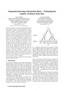
A comparison between the theoretically modelled and experimentally measured collector currents is shown in Figure 2.4. AlI measurements have been made with VCB fixed at 0 V, the gate to emitter voltage, VGE' set to +0.5 V, and the substrate voltage, VSUB ' set to -2 V below the emitter voltage. This biasing arrangement most closely resembles the conditions under which the device will be operated in the intended log-domain filter applications. The experimental values shown here represent the average of six measurements: two independent sets of measurements each from three lateral bipolar devices, each device originating in a different silicon chip. As is shown, there are significant deviations between the modelled and measured collector currents. The decrease in collector current for large values of base-emitter forward bias can be attributed to high-injection effects and parasitic base and emitter resistance. These effects will be addressed and modelled in Section 2.2.5 and Section 2.2.6. There are also significant deviations in lateral collector current at low values of base-emitter voltage, and in particular, there is a variation in the slope between the modelled and measured lateral collector current curves. This effect is difficult to model theoretically, and has been accounted for empirically using the forward emission coefficient, nF' which will be discussed in the next section. 1O-3n"='====:::E=====:I==::::::r~E~~2~7~~~~ -

Modelled le (Lateral)

Modelled le (Vertical) •

Measured Data

10-9 '----_._--J..L-..::....:...._...L.-_ _---'-0.4 0.5 0.6 0.7

' - -_ _- l -_ _- - '

0.8

0.9

V EB (V) Figure 2.4 Comparison of Eqn. (2.5) and experimentally measured collector currents

17


2.2.2 - Forward Emission Coefficient (n F) In order to compensate for the difference between the theoretical and experimental collector currents at low values of base-emitter forward bias, a second parameter, the forward emission coefficient (nF) needs to be introduced. The forward emission coefficient for a PNP transistor is defined in [22] and given by

(2.6)

and is incorporated into the calculation of collector current according to

(2.7)

In most modem bipolar devices, the value of nF is very close to unity and therefore this parameter is often omitted in device models. However, due to the relatively low doping concentration in the n-well in the 0.351l CMOS process used here, this variable must be included. This section will provide a brief explanation of the physical mechanism which gives rise to the need to model nF' and will describe the curve-fitting technique used to empirically determine nF from experimental data. When a low forward bias is placed between the base and emitter, a depletion region exists on either side of base-emitter junction. The penetration of the depletion region into the base; WDR , at a zero volt forward bias can be approximated, using equations given in [27], according to

(2.8)

where Vo represents the built-in potential of the junction (approximately 0.9 V), Vfis the forward bias across the emitter-base junction, NA and ND are the doping concentrations on the emitter and base sides of the junction respectively,

E

represents the permittivity of

silicon and q represents the charge of the electron. The resulting penetration of the lateral

18


emitter-base depletion region is approximately O.12llm for a zero-volt forward bias. The penetration will approach zero as the forward bias approaches the built-in potential. This modulation of the base, which amounts to slightly over 113 of the entire base width, is similar, although inverse, to the Early effect (see Section 2.2.4) and has been facetiously referred to as the Late effect [22]. This modulation leads the collector current to be significantly higher than would be predicted by first order theory, specifically at low values of forward bias. This effect is difficult to model accurately, particularly with the geometries involved in these lateral devices. However, because the effect is so pronounced in this case, it must be accounted for. In general, the technique for compensating for the Late effect is to empirically model the collector current using the forward emission coefficient,

np

To perform an empirical fit, Eqn. (2.7) can be rearranged into the form y =mx + b,

(2.9) and values of nF and 18 extracted from the slope and y-intercept of plot, respectively. Best fit curves for both lateral and vertical devices have been made using collector currents measured below VER

= 0.7

V. This was done to avoid including high injection effects

= 0.8 V (see Section 2.2.5). The resulting empirically calculated parameters are 18 = 1.20 x 10- 15 A and nF = 1.19 for the lateral device, and Is = 2.75 X 10- 18 A and nF = 1.03 for vertical device. The empirically which become a significant factor at approximately VER

modelled collector currents, plotted with the experimentally measured currents, are shown in Figure 2.5.

19


10-3rr========:::r"'~~~~T7~2""""--'''''''''--'~ -

Modelled le (Lateral)

Modelled le (Vertical) •

Measured Data

10-9 L-L:...-_-1..._.-!--:.::.. .._._ . L - -_ _- L_ _----'

0.4

0.5

0.6

0.7

0.8

--'-_ _---l

0.9

V EB (V) Figure 2.5 Empirical Fitting of I s and nF to experimentally measured currents

Note that the derivation given by Eqn. (2.2) to (2.5) remains a valid model for I s. Between the regions of operation in which the Late effect and the high CUITent injection and resistive effects dominate, Eqn. (2.5) can still be used to provide a reasonable estimate of I s, and the derivations in Eqn. (2.2) to (2.5) will be used in later sections to derive reasonable theoretical quantities for parameters such as I KF and

f3,

as described in

upcoming sections. However, for the purpose of accurately capturing the collector CUITent at low forward bias, the empirical values of I s and

nF

will be taken as the SPICE

parameters. These parameters will be used as the starting point in the final model optimization, to be described in detail in Section 2.3.

20


2.2.3 - Forward Current Gain (~) The maximum forward current gain,

~,

is a fundamental parameter in the operation

of a bipolar transistor. It is also a parameter which has been shown to have a significant impact on the performance of log-domain filters [32]. The value of ~ is defined simply as ratio of collector to base current,

(2.10) This section will provide a derivation of the theoretical value of ~ and will provide (by examining the resulting base currents) a comparison between the theoretically modelled and experimentally measured values of ~ for these lateral PNP devices. In most modem bipolar transistors, the dominant mechanism which gives rise to base current is the injection of minority carriers (electrons for a PNP transistor) from the base into emitter of the device [28]. In this case the theoretical value the base current can be derived in a similar manner to collector current, defined by Eqn. (2.2) to (2.5). The expression for base current can therefore be expressed by

(2.11)

where NE and WE are the doping concentration and effective width of the emitter, and nie is the effective intrinsic concentration in the emitter.

In deriving this expression, it is important to distinguish the effective intrinsic concentration, nie' used in Eqn. (2.11), from the intrinsic concentration, ni' used in Eqn. (2.5). In O.35Jl CMOS technology, the emitter is degenerately doped (that is, the doping level is sufficiently high that the Fermi level moves into the valence band for a p-type semiconductor, or into the conduction band for an n-type semiconductor). Therefore, the effective energy bandgap of a degenerately doped semiconductor is decreased by an amount Mg, leading to an effective intrinsic concentration given by

21


(2.12) where k represents Boltzman's constant and T represents temperature [26]. The effective energy bandgap in the emitter is reduced by 0.125 eV, leading to an effective intrinsic concentration of 1.68 x 10 11 cm- 3 . An expression for the theoretical value of f3 can be found by combining Eqn. (2.11) with Eqn. (2.5) to give

(2.13)

as stated in [28]. Using the dimensions and constants from Appendix, the theoretical value of f3 can therefore be calculated to be f3 = 58 for the lateral device and f3 = 8 for the vertical device. A comparison between the theoretically modelled and experimentally measured values of f3 is shown in Figure 2.6. AlI measurements have been made with VCB

= 0 V,

VGE = +0.5 V, and VSUB = -2 V, and the measurements again represent the average of three individual devices. Since the base currents for the lateral and vertical devices cannot be independently measured in practice, the base currents shown in the figure are the sum of the contributions from both devices. Therefore, the accuracy of the theoretical value of f3 is represented by the comparison of the theoretical and measured base currents. The theoretical values of f3 = 58 and f3 = 8 have been used to calculate the theoretical base current, as shown by the solid Hne in the figure. The agreement between the theoretical and measured base currents is reasonable. An improved empirical fit, based on increasing each value of f3 (while preserving the approximate ratio of lateral and vertical current gain) to f3=150 and f3=20, is shown by the dotted line in the figure. The increased empirical values will be used as the starting point in the final model optimization.

22


Note that neither curve accounts for the decrease in collector current for large values of base-emitter forward bias. This decrease can be attributed to high-injection effects and parasitic resistances, and will be addressed in Section 2.2.5 and Section 2.2.6. 10-3

•.

• -

.

.

.. .. .. .. .. .. .. .. ., ...... ..

Theoretica! 1B Ernpirica! lB

..•...

Measured lB

10-9 L - -_ _---'---------''----L--'0.4 0.6 0.5

.l...--_ _---'-_ _----L_ _- - - - '

0.7

0.8

0.9

V EB (V) Figure 2.6 Comparison of modelled and measured base and collector currents

2.2.4 - Early Voltage (VA) The Early voltage (VA) is a fundamental parameter in the operation of a bipolar transistor. It is also a key parameter which has been shown to have a significant impact on the performance of log-domain filters [32]. The Early voltage for a PNP transistor is defined as

= ( ~B' dV

c:

J-l

dW

VA

(2.14)

VCB=o

where WB represents the base width, and VeR represents the voltage across the collectorbase junction [22]. A more common expression for Early voltage is given by

23


(2.15) where ra represents the effective output resistance of the transistor. This section will provide a brief derivation of a theoretical value of VA, will describe sorne of the differences observed between the first order theory and the measured results, and will describe the technique used to empirically determine VA from experimental data. The Early voltage is used to model the variation in the width of the depletion region at the base-collector junction as a function of the base-collector bias voltage. This variation modulates the effective width of the base, giving rise to variation in cOllector current. An approximation of the Early voltage can be found by relating the derivative in Eqn. (2.14) to the base-collector junction capacitance according to

qNB ·

dW B

= cBe dV eB

(2.16)

where cBe represents the base-collector junction capacitance per unit area, which can in turn be described as CBdABe, the entire base-collector junction capacitance divided by the total effective base-collector junction area. The Early voltage can therefore be appoximated as

(2.17) as given in [28]. Using the parameters tabulated in the Appendix, the theoretical value of VA would be 2.4 V for the lateral device and 76 V for the vertical device. The expected

value for the lateral device is extremely (and somewhat unrealistically) low, but demonstrates important relationships, both resulting from the relatively low base doping of these devices. First, since the EarlY voltage is proportional to NB' the value of VA should be expected to be very low when a lightly doped n-well is used to form a base, as is the case here. Second, the EarlY voltage is proportional to WB, and therefore the "Late effect" as described in Section 2.2.2 can be expected to have an impact on the measured value of VA- This effect is demonstrated below.

24


A comparison of experimentally measured collector currents, taken at two values of collector-base voltage, is shown in Figure 2.7. The dark data points in the figure represent measured currents with VCR

= 0 V at the lateral junction, while the light data

points represent the currents with VCR

= -1

V. The lateral base width modulation which

results from the increased reverse bias is reftected in the figure by the percentage change in the lateral collector current. The percentage change can be seen to vary over the range of VER, being most pronounced at low values of forward bias (when the base-emitter

depletion region penetration is at its maximum). As a result, the measured value of VA, which would normally be assumed to be a constant, is in fact an increasing function of VER'

It is also worth noting that there is a second and somewhat surprising effect shown by Figure 2.7. The increase in lateral collector current (due to the reverse bias on the lateral junction base collector junction) is accompanied by a decrease in vertical collector current. The two transistor model of Figure 2.2 would assume the complete independence of the two devices, which is shown here not to be an entirely accurate assumption. 3

10-

""""""'"

10-4

,-.,

10-5

Q2, and C), an output compression stage (Q3 and Q4) and a IIV converter (implemented with R2). As previously mentioned, the damped integrator circuit, rather than a two input integrator, was used for testing owing to its stability over all frequencies, unlike a standard integrator which is theoretically unstable in the presence of a De input. Note that this circuit configuration does not allow for direct testing of the voltage/cuITent buffer (transistors M5 - Mg in Figure 3.5) within the integrator itself. However, initial simulations have clearly indicated that this portion of the circuitry does not impose significant limitations on the frequency response, linearity, or noise performance of the overall integrator. A symbolic representation of the test circuit is shown in Figure 3.8(b). The input compression stage in the diagram has incorporated into the integrator, as indicated in the figure.

In the testing which follows, integrating capacitors of 10 pF (on chip), 100 pF and 1 nF (placed off chip) were used, and the input and output resistors were set to 500 .Q. The current sources were implemented using PMOS and NMOS current mirrors, and the values of la, lvi' and lsh could be independently controlled with off-chip references. For current biases

from la

= lO!-lA to

100 !-lA, the value of lvi was set to be equal to la, but for CUITent biases

with la < 10 !-lA, lvi was kept fixed at 10 !-lA. A value of lsh

= 5 !-lA was

used in all tests

described in this section. The power supplies used for the simulation and testing of this circuit were nominally set to V DD = 2.5 V, AGND (analog ground)

= 2.0 V, and V55 = 0 V. The measured frequency

response of the log-domain filters was often found to be slightly improved by lowering VDD to 2.35 V to 2.45 V, and most measurements were taken from this slightly lowered voltage. The bias voltage for the cascodes in both the integrator and the V/1 circuit could be independently controlled, but was kept at 0.55 V above Vss for all tests which are described here.

59

The Design of a Log-Domain Integrator in CMOS Technology

The log-domain circuit was manufactured in

O.35~

CMOS technology. AlI circuit

simulations were performed using HSPICE and made use of the lateral PNP model developed in Chapter 2 as weIl as the

O.35~

models MOS provided by the manufacturer. AlI

measurements were made using a Hewlett Packard 3588A Spectrum Analyzer, a Tektronix TDS800 Oscilloscope, and Hewlett Packard 33l4A Function Generator. An off-chip unitygain buffer (an AD8l7 Op-Amp) was used between the filter output and the various test equipment. A microphotograph of the chip is shown in Figure 3.9(a). The total die area for a single integrator (not including CUITent sources) was

220~

x

llO~,

while the total area for on-

chip (poly/poly) capacitors in this technology was l700~2 / pp. The circuit board used for testing is shown in Figure 3.9(b).

~

Input Compression

~ VII Conversion

10

'--------....-----_..--/

~

Damped Integrator

Output Expansion IIV Conversion

(a)

I- and v3 in Figure 4.1(b) and nodes VI' Vl> and V3 in Figure 4.1(c), and therefore a relationship can be derived between cl, 12 , and c3 in the prototype and Cl' Cl> and C3 in the final implementation. Once this correspondence is found, the filter design is complete. However, in the case of the synthesis of a logdomain filter, sorne additional design steps are required in order that the non-linear nature of the log-domain integrator be taken into account. A signal flow graph representation for the log-domain integrator, which could be included in the above analysis, is discussed next.

72

The Design of Bipolar Log-Domain Filters in CMOS Technology

(a)

iZ

1 rs

+

.!.I fdt

1.fdt

1. fdt C

z

cl

3

1 rL

+ +

VI

V3 Va

(h)

--

~

Vi

Cz

Vz

(c) Figure 4.1: (a) A third order low pass LC ladder filter. (b) The corresponding signal flow graph. (c) An active flUer implementation based on operational simulation of original LC ladder.

73


4.1.2 - Operational Simulation for Log-Domain Filters The general structure of a log-domain ceIl, whether it be an integrator or an entire log-domain filter, is shown in Figure 4.2(a). The EXP(x) and LOG(x) operators defined in Eqn. (3.6) and (3.7) have been explicitly shown with symbols in the figure. The diagram is simple, and yet demonstrates an important point: that the input and output signaIs of this cell are logarithmically compressed, though the function being implemented, denoted by h(t), has a linear representation. ConceptuaIly, the cell can be thought of as performing the operation h(t) by first exponentially expanding the signal at the cell input, implementing the desired linear function, and then logarithmically compressing the signal at the cell output. A signal flow graph representation for a log-domain integrator which demonstrates this order of operations is shown in Figure 4.2(b). Note that this signal flow graph conforms to the log-domain integrator equation defined in Eqn. (3.13). To continue with the example of the third order low pass filter of the previous section, the original signal flow graph can now be modified to include the log-domain integrator. This modification is shown in Figure 4.3(a). Observe that a natural cancellation of the majority of LOG(x) and EXP(x) operators naturally occurs, simplifying the filter

h(t) L

~

~

EXP operator

D

LOG operator

(a)

If

la ' - (.)dt vT C

(b) Figure 4.2: (a) A signal f10w graph representation for a generallog·domain cell. (b) A signal f10w graph representation of the log·domain integrator.

74


design considerably. Due to cancellation, an entire log-domain filter can in general be implemented using only a single logarithmic compression circuit at the filter input and a single exponential expansion circuit at the filter output, and as shown by the circled LOG(x) and EXP(x) blocks in Figure 4.3(a). A circuit implementation of this signal flow graph is given in Figure 4.3(b). Once a log-domain circuit representation for the original prototype LC ladder has been created, the variables from the LC prototype filter can be mapped to the final circuit implementation. Finding this correspondence represents the final step in the synthesis of a log-domain filter. The details of mapping the variables from the prototype to the final circuit are best demonstrated by example, as will be provided in the next section.

D

o

1

LOG EXP

(a) VII and Input Logarithmic Compression

Output Exponential Expansion and IIV

(b)

Figure 4.3: (a) A third order low pass filter log-domain signal flow graph. (b) A log-domain filter implementation of the signal flow graph.

75


4.2 - The Design of Second and Third Order Log-Domain Filters The following section will provide an overview of the synthesis of a biquadratic and a third order elliptic filter. Each of the filters designed in this section will be the subject of the experimental tests presented later in this chapter. The material presented here has been adapted from [1], which provides further details on the derivation and synthesis of these filters.

4.2.1 - A Low Pass Biquadratic Log-Domain Filter A low pass biquadratic filter can be designed starting with the LC prototype filter shown in Figure 4.4(a). This circuit has a transfer function which can be expressed as

=

1/(lc) 2

s + s/(rc) + l/(lc)

.

(4.4)

By comparing this equation with the standard biquadratic form, 2

R(s) =

k . Wo

(4.5)

expressions for the natural frequency, wO ' the quality factor, Q, and the gain, k, of the LC circuit can be determined, and are given by

k

= 1.

(4.6)

To simplify matters, the resistance, r, will be set to unity for the analysis which follows. The set of equations which completely define the operation of the biquadratic prototype tilter can be expressed as

(4.7)

and

(4.8)

76


A signal flow graph can be generated from these equations, as shown in Figure 4.4(b). By adding LOG(x) and EXP(x) cells to the diagram, and by mapping the variables names 1] and V 2 to lin'

V1

and

Vz,

Vi,

a corresponding log-domain signal flow graph can be

generated, as shown in Figure 4.4(c). In this case, the set of equations can be rewritten as

(4.9) (4.10)

and

A log-domain circuit implementation of the signal flow graph is shown in Figure 4.4(d). Note that the input compression stage has been combined with the first integrator and is implemented in a manner similar to that shown previously in Figure 3.8(b) for the damped integrator. The circuit equations at nodes

V1

and

Vz can be

expressed as

(4.11)

and

la 1 f = -' _. {EXP(Vd -EXP(Vz)}dt. v C

A

A

EXP(Vz)

A

z

T

(4.12)

From a comparison of Eqns. (4.9) to (4.12), the relationship between l, c, Cl> and C2 can be expressed as

(4.13)

Finally, combining these equations with those listed in Eqn. (4.6), the natural frequency, quality factor and gain of the filter of the log-domain filter can be determined to be

la 00

0

= vT

.

1 JC C l

z

'

Q=~,

k

= 1.

(4.14)

By selecting la, Cl> and C2 , the design of the log-domain filter is complete. A simplified circuit schematic for the complete biquadratic filter is shown in Figure 4.5.

77


(a)

(b)

1.

ln

~

EXP

D

LOG

(c)

lntegrator # 1

lntegrator # 2

Output Exponential Expansion and IN

Vaut

(d)

Figure 4.4: (a) The prototype biquadratic Le fllter. (b) The prototype signal f10w graph. (c) The log-domain signal f10w graph. (d) The log-domain circuit implementation.

78


(Damped) Integrator # 2

~~ VII Conversion Input Compression Output Expansion IIV Conversion

Integrator # 1

Figure 4.5: A simplified schematic of the final biquadratic filter implementation.

4.2.2 • A Low Pass Third Order Elliptic Log.Domain Filter A low pass third order elliptic filter can be designed starting with the

Le

ladder

prototype filter shown in Figure 4.6(a). Once again, to simplify the analysis, the values of the input and output resistance in the prototype have been set to unity. The set of equations which completely define the operation of the filter can be expressed as

(4.15)

(4.16)

and

(4.17)

79


These equations can be manipulated in order to simplify the derivative terms, resulting in

(4.18)

(4.19)

(4.20)

and

A signal flow graph can be generated from these equations, as shown in Figure 4.6(b). By adding LOG(x) and EXP(x) cells to the diagram, and by mapping the variables names VI>

h, V 3 and Vout to

~,

lin' VI, V 2, V 3, and lout, a corresponding log-domain signal flow

graph can be generated, as shown in Figure 4.6(c). In this case, the set of equations can be rewritten as

(4.21)

EXP(V 2 )

= t-. f{EXP(Vd- EXP (V3)}dt

(4.22)

,

2

and

(4.23)

Note that the log-domain filter cannot be directly implemented from the above equations, since we do not have a functional block analogous to a log-domain differentiator. However, as is the case in other active filter technologies, the realization of the differentiator can be approximated by placing a single capacitor placed between the VI and

V3, nodes of the circuit [1].

(Indeed, a floating capacitor placed between the VI and

V 3 nodes was used to generate the zero in the transfer function of the original Le ladder prototype.)

The

corresponding

log-domain

filter

implementation

is

shown

in

Figure 4.6(d).

80

The Design of Bipo1ar Log-Domain Fi1ters in CMOS Techno1ogy

The circuit equations 1 generated from this figure are given by

1

= -J . C C ' 0

A

EXP(V 1)

vT

1+ 4

f

{

vTC4 d } J. -EXP(V 1) - EXP(V 2 ) + - J - ' -d (EXP(V 3 » dt A

A

zn

A

0

t

,

(4.24)

(4.25)

and

1 10 EXP(V 3 ) = v ' C + C ' T 3 4 A

f

{

A

A

EXP(V 2 ) -EXP(V 3 ) +

d vT4 C } T' d/ EXP (V 3 » dt. A

(4.26)

From a comparison of Eqns (4.21) to (4.26), the relationship between the circuit elements can be expressed as

(4.27) As the final step, the values of the capacitors and inductors for the prototype filter would be determined based on the desired fiIter specifications. For an elliptic fiIter, these can be read from fiIter tables [35] or determined with computer-aided design tools. Once these values have been mapped to the log-domain fiIter implementation according to Eqn. (4.27), the filter design is complete. A simplified circuit schematic for the complete third order elliptic filter is shown in Figure 4.7. The biquadratic and elliptic fiIters described above have been fabricated and tested, and an experimental characterization of these fiIters will be provided in the next section. It will be demonstrated that fiIters with desired responses can be generated using the synthesis methods presented above.

v

T 3 . h ave b d usmg ' an approxlmatlOn " 1. Th ese equatlOns een generate th at e VI/V = e /v]' , as described in detail in [1], and is the reason why the realization of the differentiator function is on1y"approximate".

81


1

+ 1 Vout (a)

1

1

DLaG

rza EXP

Integrator #2

Integrator

#4

V3

VI Integrator # 1

Integrator # 3 Output Exponential Expansion and llV

T--

C4

CI (d)

C

3T --

Vaut

Figure 4.6: (a) The prototype elliptic Le ladder fllter (b) The prototype linear signal flow graph (c) The log-domain signal flow graph (d) The log-domain-circuit implementation

82

Integrator # 2

VII Conversion Input Compression

1

(Damped) Integrator # 4

Il

1

IIV Conversion Output Expansion

~~ 11

,

~

J

II

~ C3

T

---3

:::>"

(1)

ti

(1)

f!l.

6o

S po El"

~

~

~ (Damped) Integrator # 1

Integrator # 3

'"S· n s:::

oCIJ ---3

Figure 4.7: A simplified schematic of the final elliptie fiUer implementation 00

w

(1)

~

0'


4.3 - Experimental Results This section will discuss the experimental performance of biquadratic and elliptic low pass fiIters fabricated in 0.35!-t CMOS technology. The three categories of tests have been used to characterize the fiIter performance: frequency response, linearity, and noise performance. In the final section of this chapter, a comparison between the measured performance versus other fiIters described in the literature will be provided. First, the circuit under test and the test conditions will be described.

4.3.1 - Description of the Log-Domain Filter Test Circuits The biquadratic and elliptic fiIters used in testing are shown in Figures 4.5 and 4.7. These circuit diagrams have been simplified for visual clarity, though aIl measurements have been made using the complete integrator circuitry shown in Figures 3.5 to 3.7. Several different ranges of capacitor values for both types of filters were used, and are listed in Table 4.1. The theoretical cut-off frequencies (based on ideal transfer functions) for bias currents of 10

= 100 !-tA have been listed in each case. The biquadratic

filters (Filter #1 - #3) have been designed to have a constant quality factor of

Ji, and were

implemented with external capacitors. The elliptic fiIters (Filters #4 - #6) have each been designed to have a maximum passband ripple of 1 dB and a stopband attenuation of 30 dB. Filters #5 and #6 were implemented with integrated capacitors, while Filter # 4 was implemented with external capacitors. The input and output resistors for the biquadratic filter were set to 500 Q, while the input and output resistors for the elliptic fiIter were set to 500 ,Q and 1 k,Q respectively. The doubled value of output resistance of the elliptic fiIter was used to compensate for the 6 dB passband attenuation present in original LC ladder prototype filter. The values of 10 , Ibl , Ib 2> Iyi , and Ish could be independently controlled with offchip references. For current biases from 10 = 10 !-tA to 100 !-tA, the values of Ibl , Ib2 and I yi were set to be equal to 10 , but for current biases with la < 10 !-tA, Ibl Ib2 , and Iyi were kept fixed at 10 !-tA. A value of I sh = 5 !-tA was used in aIl tests described in this section. 84


Table 4.1 - Capacitor values used for biquadratic and elliptic fllter testing Capacitor Values

Theoretical Cut-Off Frequency (10 = 100/-lA)

Cl = 200 pF, C z = 100pF

4.5 MHz

Cl = 100pF,Cz =50pF

9.0 MHz

Filter # 3

Cl = 50 pF, C z = 25pF

18 MHz

Filter # 4

Cl = 275 pF, Cz = 125 pF, C3 = 275 pF, C4 = 50 pF

4.0 MHz

Cl = 110 pF, Cz = 50 pF, C3 = IlOpF,C 4 =20pF

10 MHz

Cl = 44 pF, Cz = 20 pF, C3 = 44 pF, C4 = 8 pF

25 MHz

Filter Type

Filter # 1

Filter # 2

Filter # 5

Biquadratic

Elliptie

Filter # 6

The power supplies used in testing the circuit were VDD ground)

= 2.0 V,

and Vss

= 0 V.

= 2.5 V, AGND (analog

The frequency response was once again found to be

slightly improved by lowering the VDD to between 2.35 V and 2.45 V, and most measurements were taken from this slightly lowered voltage. The bias voltage of the cascoded transistors within the integrator were kept at 0.55 V above Vss for all tests described here. The log-domain filters were manufactured in 0.35J.1 CMOS technology. A microphotograph of the biquadratic and elliptic filters are shown in Figure 4.8. The total die areas for the biquadratic and elliptic filter (not inc1uding CUITent sources) were 340J.1 x 11OJ.1 and 515J.1 x 11OJ.1 respectively, and the total area for on-chip (poly/poly) capacitors in this technology was 1700J.12 / pp. AlI measurements were made using a Hewlett Packard 3588A Spectrum Analyzer, a Tektronix TDS800 Oscilloscope, and Hewlett Packard 3314A Function Generator. The circuit boards used for testing were similar to that shown previously in Figure 3.9(b).

85


(a)

(b)

Figure 4.8: (a) A mierophotograph of the biquadratie flUer and associated circuitry (b) A mierophotograph of the elliptie flUer and associated circuitry

4.3.2 - A Biquadratic Low Pass Filter This section will describe the measured performance of a low pass biquadratic logdomain filter, and will begin with an examination of the filter frequency response. The experimentally measured response of the filter is shown in Figures 4.9 and 4.10. In the first figure, the filter capacitance has been held constant while the bias current 10 has been varied from 1 /lA to 100 /lA. In the second figure, a constant current of la

= 50 /lA has

been used, while the filter capacitor values have been varied. The simulated response has been inc1uded in the figure for comparison. The frequency response was very well predicted by simulation, the most significant deviation being the small amount of peaking observed when large currents and relatively small capacitances were used for the filter. Though relatively large off-chip capacitors were used for these tests, a maximum 3-dB frequency of 5.0 MHz was observed, and the ability to tune this eut-off frequency of the filter by almost two decades using the bias current, la, is c1early demonstrated in Figure 4.9. 86


0 -5 ,-"

ÇQ

""0

-10

'-"

.....l=:

~

d

-15 -20

.

... . . . . . .,', . ..

HSPICE Simulations -25

Measured Results

_30'--~~~~-"-'--~~~"""""'-~---"--~~'-'-~~~~.........c_---"-I.....J

1~

1~

1~

1~

1~

Frequency (Hz) Figure 4.9 Frequency response of biquadratic flIter # 1, 10

=I/lA =100 /lA.

5 0 -5 ,-"

ÇQ

""0

Filtef# l

-10

'-"

.....l=: ~

d

-15 . Filter # 3

-20

HSPICE Simulations

-25 -30

Measured Results 5

10

Frequency (Hz) Figure 4.10 Frequency response of biquadratic flIter # 1 - # 3, 10

=50 /lA

87


The overall linearity of the filter was characterized using measurements of both total harmonie distortion and third order intercept points, and the results of these tests are

= 10 !-lA and an input signal of 100 kHz was used in each case. The THD of the filter at lin =0.51 was -43.1 dB and the output shown in Figures 4.11 and 4.12. A bias CUITent of 10

0

third order intercept point was measured to be 149 !-lApeak ' Both values are close to, though slightly lower than, the cOITesponding values measured for the single damped integrator in Chapter 3, a result which reasonable since the filter order and circuit complexity have been increased. The noise performance of the filter was characterized using measurements of SNR, dynamic range, and output noise CUITent. The SNR of Filter # 2, with 10 set to 10 !-lA and with a measurement bandwidth of 800 kHz, is shown in Figure 4.11. The maximum value of SNR was 39.6 dB, and the total dynamic range, as defined in Chapter 3, was 35.2 dB. The total output noise CUITent over the measurement bandwidth was 121 nA rms ' By increasing the bias CUITent to 50!-lA, both the SNR and dynamic range could be improved by several decibels. However, as in the case of the damped integrator, the measured noiserelated performance is significantly lower than anticipated, suggesting that there may be significant room for improvement in the test and measurement set-up. A summary of aIl biquadratic filter measurements is given in Table 4.2. An important note should be made with regard to difficulties which arose from the presence of multiple operating points within these filter circuits. As described in [17], CMOS log-domain filters which contain sorne form of positive feedback loops within their topologies can suffer from this effect, which can take the form of several circuit nodes settling to unintended states. This behaviour has been observed experimentally in both the biquadratic and elliptic filters described in this work. SpecificaIly, for circuits in which capacitances were placed off-chip (in which internaI circuit nodes were directly accessible) the voltages at these capacitive nodes were often observed to settle to undesired voltages. Under such conditions, the filter is inoperable.

88


60

20

---

40

Measured SNR Measured THD 0

,-...,

......

o:l

'

..

. ...

~

. .

,-...,

.'

~ '-"

"'d

'-"

~

..

20

-20

Z

Q

::c: E--

CZl

0

..

-20

-60 10-4

10-7

Input CUITent (Apeak) Figure 4.11: SNR and THD for flUer # 2, 10

=IOIlA, lin =100 kHz, BW =800 kHz

10-3 """"~~CC-=~~~~"""""~""""'~~~-cT7T=r.""""""""""'~,.".,.,~~cr.-s", ......... ,.. . .. " ..... , ... , •.•••.•

"

......

_"0'

.... , ..•.. , . . . . . . ,

.... :.:OIP.1 == :l49l-tA:.

•.•• ,

•. /,.,

; .. ;

.:

.

: ': : ~ :.:

................ ... , .........", "..", '...,

.,

"·'1 ·:::1

.

..- .... ,., ....

·1·· . '1

: .:.,,:.;.;.',

,,:,,1 .. , ':':1

::::1 .... :.,,:.:' . . . .

'"

.

-,"

'" '.'

.

........ 1. 1 .

';"

.

.: T 1

. .•

.

.

ï .. ': .... , .. '.'. ;"1 ,,; ....... ' ::

"',::::'1 ~ .Measured Data ..

.

r:

1.. .

" "., ': ~ .' " ,." ,,: " ,,:' i' ' ......

1

:: :j:'::'

...." ".. ,.,

.

, .

Input CUITent (Apeak) Figure 4.12 Third order intercept points for flUer #1, 10

=IOIlA, lin =100 kHz

89


Table 4.2 • A summary of the biquadratic fiUer performance

Parameter

Bias Current

Conditions

Experimental Results

Frequency Range

la = 1J..lA - 100 J..lA

Filter #1

26 kHz - 2.2 MHz

(f3dB )

la =50 J..lA

Filter #1 - #3

1.6 MHz - 5.0 MHz

THD

la = 10 J..lA

Filter # 1, lin = 0.5 la at 100 kHz

-43.1 dB

Third Order Int.

la = 10 J..lA

Filter # 1, lin = 100 kHz

149 J..lApeak

= 10 J..lA la =50 J..lA la = 10 J..lA 1 = 10 J..lA 1 = 50 J..lA la = 10 J..lA 1 = 100 J..lA

Filter # 2, BW = 800 kHz

39.6 dB

Filter # 1, BW = 2.0 MHz

43.5 dB


121 nArms

0


35.2 dB

0

Filter # 1, BW = 2.0 MHz

43.9 dB

10

MaximumSNR Noise CUITent

Dynamic Range Power per pole (simulated)

0

191 J..lW Filter # 1 2.09mW

Two methods were used in an attempt to alleviate the problem: first, the switching or cycling of various filter bias currents could be used to push the filter through various states, eventually leading to the desired operating point. This method does not appear to lend itself to any fixed start-up procedure and requires a great deal of patience. However, for aIl but the lowest levels of current biasing, circuits could be successfully started using this method. The second method, which was implemented on the most recent chip submissions, involved the inclusion of switches which could be used to temporarily force various internaI nodes to predetermined voltages. This method was not found to be very effective, since the filters could not function with switches tumed on, and would generally retum to previous undesired states once switches were tumed off. The first of the two methods was generally found to be preferable.

90


A detailed investigation of the locations and origins of the multiple operating points of these biquadratie and elliptic filters was not undertaken, though it would be strongly recommended that this issue be examined if research using this CMOS circuit topology is continued in the future. A method for determining the existence of multiple operating points is described in [17], and a technique which may possibly eliminate such operating points is described in [36].

4.3.3 - A Third Order Elliptic Low Pass Filter This section will describe the experimentally measured performance of a low pass elliptic log-domain filter, and will begin with the filter frequency response. The experimentally measured response of the filter is shown in Figures 4.13 and 4.14. In each plot, the bias CUITent has been held constant at 10 /-!A and 100 /-!A respectively while the filter capacitance has been varied. The simulated elliptic frequency responses have been included for comparison. The overall response of the elliptic filter was far less ideal than in either the damped integrator or the biquadratic filter cases shown previously. First, it should be mentioned that the elliptic filter was not observed to function at low values of bias CUITent due to the existence of multiple operating points as described in the previous section. In addition, there was an unexpected peak in the response at approximately 20 MHz which has masked the location of the zero in the elliptic transfer function for la

= 100 /-!A

(though based on the slope of the

response, the zero must have been present). The measured stopband attenuation, designed for 30 dB, was measured to be between on1y 16 and 28 dB. There is also significant peaking in the response near the cut-off frequency, though such peaking can be significantly reduced simple using simple techniques such as resistive lead compensation. Despite these issues, the two plots demonstrate that an elliptic filter can be implemented using the circuitry and methods described in this work, and that the filter can be tuned by means of bias CUITent or filter capacitance as expected. The implementation of an elliptie function is significant, since it verifies that both the poles and zeros can be accurately placed, a testament to the potential of this CMOS filter design approach and technique. Aiso note that the measured maximum cut-off frequency of the filter was 10 MHz, a figure very difficult to achieve using subthreshold MOSFET devices.

91


-10 ,,-...

Filter.# 4

PO

"'0

"-' ~ ......

. FiIter # 5

-20

C\l

c;

Filter # 6·

-30

HSPICE Simulations Measured Results

Frequency (Hz) Figure 4.13 Frequency response of elliptic fllter # 4· # 6, 10 = 10 /-lA

o -

-10

...... " ....

,,-...

E§ "-' ~

......

C\l

c;

-20

-30

HSPICE Simulations 1 1 1 1

Measured Results -40 5 10

Il 1\

10

6

7

10

8

10

Frequency (Hz) Figure 4.14 Frequency response of elliptic fllter # 4· # 6,1 0 = 100 /-lA

92


Next, the overall linearity of the filter was characterized using measurements of both the total harmonic distortion and the third order intercept points, and the results of

= 10 IlA and an input signal of 100 kHz was used in each case. The THD of the filter at lin = 0.51 was

each of these tests are shown in Figures 4.15 and 4.16. A bias CUITent of 10

0

measured to be -39.6 dB and the input and output third order intercept points were measured to be 116 IlApeak and 55 IlApeak respectively (the difference between the input and output points reflecting the fact that the output CUITent gain of the filter is approximately 0.5). Both the THD and input third order intercept points show a slight reduction from the biquadratic filter measurements, as should be expected. The noise performance of the filter was characterized using measurements of SNR dynamic range, and output noise CUITent. The SNR of Filter # 6, with 10 set to 10 IlA and a measurement bandwidth of 1.5 MHz, is shown in Figure 4.15. The maximum value of SNR was 31.2 dB, and the dynamic range was 34.1 dB. The output noise CUITent over the measurement bandwidth was 134 nArms ' The total noise CUITent was slightly increased with respect to the noise current for the biquadratic filter, and as a result the measured values of SNR and dynamic range show a reduction from those given in the previous section. The value of SNR has been further reduced from the biquadratic case due to the elliptic filter CUITent gain of being 0.5 rather than unity. By increasing the bias CUITent to 50IlA, the SNR and dynamic range could once again be improved by several decibels. As

in previous cases, the measured noise-related performance is significantly lower than anticipated, and there may be significant room for improvement in the test and measurement set-up. A summary of the elliptic filter measurements are listed in Table 4.3. The performance of the biquadratic and elliptic filters have been characterized, and a comparison to the performance of other log-domain filters described in the literature will now be provided.

93


40

20

--

Measured SNR Measured THD

,-....

,-....

~

~ "-"

"-"

zr.n~

a

0

::c: E--

-20

-40 10-7

10-6

-60 10-4

10-5

Input CUITent (Apeak) Figure 4.15: SNR and THD for fllter # 6,1 0 = 10f-lA, lin = 100 kHz, BW = 1.5 MHz

The Development ofBipolar Log-Domain Filters in ... - Semantic Scholar

The Development ofBipolar Log-Domain Filters in ... - Semantic Scholar

Suggest Documents

Bloom Filters in Probabilistic Verification - Semantic Scholar

RF SAW Filters - Semantic Scholar

Development of Optical Filters Based on ... - Semantic Scholar

Carbon nanotube filters - Semantic Scholar

information filters and their implementation in the ... - Semantic Scholar

Filters for Semantic Service Composition in ... - Semantic Scholar

Exploring collaborative filters: Neighborhood ... - Semantic Scholar

Parametric Bayesian Filters for Nonlinear ... - Semantic Scholar

Order Statistic-Based Nonlinear Filters - Semantic Scholar

Analytical Design of FIR Filters - Semantic Scholar

Recursive Gaussian Derivative Filters - Semantic Scholar

Mixture Kalman Filters 1 Introduction - Semantic Scholar

Improved Fully Differential Analog Filters - Semantic Scholar

Modified repeated median filters - Semantic Scholar

Recursive weighted median filters admitting ... - Semantic Scholar

Sequential clustering with particle filters ... - Semantic Scholar

Agentized, Contextualized Filters for Information ... - Semantic Scholar

DEVELOPMENT IN THE USE AND ... - Semantic Scholar

Coordination in Software Development: The ... - Semantic Scholar

Supporting Application Development in the ... - Semantic Scholar

The NM23 family in development - Semantic Scholar

Coordination in Software Development: The ... - Semantic Scholar

in Software Development - Semantic Scholar

Issues when designing filters in messaging systems - Semantic Scholar