decomposition, based on NOR functions, is indeed canon- ical: A function can be ..... We call pushing z into A the operation of moving z from the support of F (as ...
The disjunctive decomposition of logic functions Maurizio Damiani Synopsys, Inc. 700 E. Middlefield Rd. Mountain View, CA 94043
Valeria Bertacco Computer Systems Lab. Stanford University Stanford, CA 94305
Abstract
Algebraic factoring [6] is a form of disjunctive decomposition: one attempts to decompose a 2-level cover of F into a product G � H , where G and H have no variables in common. Factoring is a powerful step in passing from a Boolean cover to a multiple-level representation in multiple-level logic synthesis [7]. Recently, decomposition has also been considered in the context of technology mapping ([8]) and canonical Boolean function representation ([9, 10]). In [10] it was in particular shown that a simple form of decomposition, based on NOR functions, is indeed canonical: A function can be decomposed into the NOR of disjoint-support components in a unique way. This result was used to develop a normal form (MLDDs) for Boolean functions based on Shannon- and NOR- decompositions. Algorithms for translating BDDs into MLDDs and for the direct manipulation of MLDDs were also presented. These algorithms are very efficient in terms of CPU time, as the decomposition of a function is inferred locally from that of the two cofactors. Moreover, the decomposition of cofactors of complex functions often evidenced common subfunctions, whose sharing resulted in memory savings with respect to BDDs. The resulting netlist, however, is not particularly appealing, because of the restriction to NOR decompositions only. In this paper, we provide the following contributions. First, we present new results on canonicity. We introduce prime functions, functions that cannot be further decomposed. Some such functions are, for example, 2-input logic functions, the 2-input MUX function, and all non-trivial symmetric functions. Clearly, when we attempt the decomposition of a function F as F = L(A; B; � � �) we only need consider prime functions L. We prove that logic functions can be classified as follows: 1. F is prime; 2. F is decomposable using a binary associative operator X (X = OR,AND,XOR) of disjoint-support functions:
In this paper we present an algorithm for converting a BDD representation of a logic function into a multiple-level netlist of disjoint-support subfunctions. On the theoretical side, we show that the algorithm takes at most quadratic time in the size of the BDD and that the resulting netlist retains the canonicity properties of the original BDD. Experimentally, we found the algorithm to be extremely fast, taking at most a few minutes for the most complex benchmark circuits. The resulting netlist is also often better than what achieved by conventional synthesis tools.
1 Introduction. A
disjunctive decomposition of a function a partitioning of the inputs x1 ; � � � ; xn in disjoint subsets, so that F can be given a multiple-level representation as :
F (x1 ; � � � ; xn ) is
F (x1 ; � � � ; xn ) = G(A(x1 ; � � � ; xA ); B (xA+1 ; � � � ; xB ); � � �) (1) Discovering a disjunctive decomposition of F such as in Eq.
(1) is beneficial in several respects: First, a disjunctive decomposition evidences some parallelism in the (hardware or software) computation of F : one can evaluate the component functions A; B; � � � ; in parallel, as they share neither variables nor intermediate results. Second, a disjunctive decomposition suggests implicitly a clustering of inputs and functions so as to reduce the amount of interconnect: Cells can be designed so as to compute separately G; A; B; � � �. The designer can concentrate on the optimization of the cells implementing the individual functions, and the routing problems are simplified as only one wire needs be brought out of each cell. The reduction of interconnects is of increasing importance with the advent of deep submicron technology, where the interconnect delay tends to dominate the overall circuit performance. Eventually, we observe that a disjunctive decomposition can be beneficial also for other logic functions representations, namely BDDs [1, 2], since it offers implicitly a good partial ordering of the primary inputs for BDD construction. Previous work and contributions of this paper. Decomposition algorithms are a classical research subject of switching theory. Exhaustive search procedures have been presented in [3, 4, 5], and were efficient for circuits with six or fewer inputs [4]. At the time, decomposition was regarded as the main path to multiple-level logic synthesis.
3.
F = X (A0 ; A1 ; � � � ; An ) (2) In this case, F cannot be decomposed using any other function L; moreover, the functions Ai are identified uniquely (modulo permuttion, complementation) provided they cannot be further decomposed by X ; F is decomposable using a prime function L of three or more inputs:
F = L(A0 ; � � � ; An ); n � 3 1
(3)
In this case, also L and the functions Ai are identified uniquely (modulo permulations/complementations), that is, no other prime function L can decompose F .
lowing two results indicate that also the functions in are essentially unique:
F=L
Theorem 2. If a function F is reducible by L, with jSL j � then the functions F=L are unique, up to permutations and complementations. 2
3,
The above results indicate essentially the uniqueness of a disjunctive representation of F . We then present an algorithm for inferring the disjunctive decomposition of F from the BDD representation. The algorithm is fast, as it is based on the local inference of the decomposition of a function F from that of its cofactors. It is worth noting that the success in identifying a decomposition does not depend on the topology of the BDD representation (as affected, for instance, by the variable ordering). Hence, the method differs in scope from topological techniques such as those presented in [11].
Theorem 3. If a function F is reducible by L, with jSL j = X . The operator X decomposing F is unique; moreover, the functions A; B; � � � in the decomposition 2, then it is reducible by an associative operator
F = X (A; B; C; � � �)
are also unique, provided they are not further decomposable by X . 2 Theorem (3) in particular indicates that if a function can be decomposed as the (say) XOR of two disjointsupport components, then no other operator (AND, OR) decomposes it. Moreover, the component functions are identified uniquely, provided they’re not further decomposable. Since AND-decomposable functions are complements of OR-decomposable ones, Theorems (1 - 3) allow us to ultimately classify logic functions as follows: 1. prime; 2. decomposable by a prime function L; jSL j � 3; 3. XOR-decomposable; 4. OR-decomposable; 5. complements of OR-decomposable functions.
F
2 Disjoint-support decompositions. This section provides the relevant definitions and theoretical results. Let B denote the Boolean set f0; 1g. A Boolean function is a mapping F : B n ! B . We say that a function F depends on a variable xi if @F=@xi is not the constant function 0. We call support of F the set SF of variables F depends on. The size of SF is the number of its elements, and it is indicated by jSF j. We say that two functions F and G are disjoint-support if they share no variables, i.e. SF \ SG = �. We say that a function F is NP-equivalent to a function G if it can be obtained from G by a permutation / complementation of some of the inputs of G. Hereafter, lower-case and upper-case letters will denote Boolean variables and functions, respectively.
3 BDD-based logic decomposition.
Definition 1. A function F (x1 ; � � � ; xn ) is said to be reducible by L if it can be expressed as the composition of other non-constant disjoint-support functions A; B; : : :: F = L(A; B; � � �) (4) F is said to be prime if it cannot be decomposed by any L. If Eq. (4) holds, we say that a function L reduces F . We denote by F=L any set of functions fA; B; � � �g satisfying Eq. (4). 2
We now present algorithms for mapping a BDD representation of a function F into a multiple-level netlist of disjoint-support components. We will first describe the data structures employed for the function representation, and then present the actual relevant procedures. A disjunctive decomposition could be represented just by introducing hierarchy in an ordinary BDD-based representation. This is obtained by allowing splitting function instead of a splitting variable.
It is worth noting that the set F=L is, in general, not unique. Consider, for example, the function F = x1 + x2 + x3 and a function L = a + b. Then one can write (for instance) F = L(x1 ; x2 + x3 ) or F = L(x1 + x2 ; x3 ). The two options result in F=L = fx1 ; x2 + x3 g and F=L = fx1 + x2 ; x3 g, respectively. We also observe that if L reduces a function F , then any other function NP-equivalent to L also reduces F . Moreover, L reduces F if and only if L0 reduces F 0 . We now present the main theoretical contributions of this paper. For reasons of space, the proofs have been omitted from the paper.
Example 1. Consider the function F = MAJORITY (a � b; cd + e; ITE (fg; h; i)). F has the following disjointsupport representation: F = MAJORITY (G; H; I ) (6) G = a�b (7) H = L+e (8) I = ITE (M; h; i) (9) L = cd (10) M = fg (11) Fig. (1) shows the representation of F . 2
Theorem 1. Consider an arbitrary function F (x1 ; � � � ; xn ), and a prime function L(a; b; � � �). Suppose L reduces F : F = L(A; B; C; � � �); (5) Then F is reduced only by functions M that are NPequivalent to L. 2
This representation, however, does not fit entirely our purposes, because complex functions generally lack significant decompositions, and consequently do not take advantage of hierarchy. It is often the case, however, where a function, albeit lacking a decomposition, has decomposable cofactors. It is then better to represent the function by Shannon decomposition, using the decomposed forms of the cofactors. A function is then here represented by two
The above Theorem states that the prime function reducing L is unique, modulo syntactic transformations. The fol2
Viceversa, suppose F0 ; F1 are expressed as
a
F
F0 = L0 (A0 ; B; � � �); F1 = L1(A1 ; B; � � �) jF0 =L0 \ F1 =L1j = jF0 =L0 j ? 1 = jF1 =L1j ? 1 (13) (that is, F0 =L0 and F1 =L1 differ in exactly one element, A1 in place of A0 ) and suppose L0 (A0 = 0) = L1(A1 = 0); L0(A0 = 1) = L1 (A1 = 1); (14) then it is easy to verify that F can be written as in Eq.(5), where L = L0 and A = A0 z + A1 z . The compliance of F0 ; F1 to Eqs. (13) is easily tested
b 0
1
G c
L H
H 0
0 0
0
1
e
1
I
1
d 0
1
1
M
f
0
h
0
i
0
1
0
g
1
0
from their decomposition lists. The compliance to Eqs. (14) is tested by computing the four cofactors and verifying their identity. Example 2. Consider again the function F = MAJORITY (a � b; cd + e; MUX (fg; h; i)), and its cofactors F0 = F (g = 0); F1 = F (g = 1). We consider available the representations of the cofactors : F0 = MAJORITY (G; H; h) (15) G = a�b (16) H = L+e (17) L = cd (18) F1 = MAJORITY (G; H; N ) (19) N = MUX (f; h; i) (20) Their decomposition lists are (G; H; h) and (G; H; N ), respectively. They differ in exactly one element, namely, N instead of h. We then check if Eqs. (14) hold. This check can be carried out by computing F0 (h = 0); F0 (h = 1); F1 (N = 0); F1 (N = 1), and verifying the identities
1
Figure 1. ITE-dag representation for Example (1) distinct data structures, namely, one representing its decomposition structure (i.e.decomposition tree), and the second its proper logic functionality.
4 Constructing the decomposition. The algorithms of this paper aim at constructing a representation as in Fig. (2) from the BDD of F . F
G
Prime 0
G
H
Xor a
e Var
b
And
H
H
I
Or L
1
0
Prime
1
I
i
M
0
And
h
1
Var
F0 (h
Var
Var
Var
1).
0
c Var
d Var
1
g f
h Var
i
Var 0
1
0
= 0) =
F1 (N
; F0 (h
= 0)
= 1) =
F1 (N
=
Indeed, both these identities hold in our case. We then form a representation of the function I = g 0 h + gMUX (f; h; i) and construct a representation of F as MAJORITY (G; H; I ). 2
M
1
Case 2. Suppose z belongs to the support of a nontrivial function (say, A, with jSA j >= 2), but such that exactly one of A0 ; A1 is constant (say, A1 = 1). The cofactors are: F0 = L(A(z = 0); B; � � �); F1 = L(1; B; � � �) (21) In the expression of F1 one of the arguments of L is a constant. Hence, F1 is decomposed no longer by L but by some other prime function. Notice, however, that the functions B; � � � will be in the decomposition tree of F1 . Moreover, the two cofactors still have the property F0 (A = 1) = F1 . Viceversa, suppose F0 ; F1 are decomposable as F0 = L0 (A; B; � � �); F1 = L1 : (22) and that one can find an element in the decomposition list of F0 (say, A) such that: L0 (A = 1) = L1 ; (23) one can then write F = L0 (A + z; B; � � �): (24) The inference of the decomposition for F is slightly more complex than the previous case. First, we need to identify all the possible candidate functions in the decomposition list of F0 . The functions not appearing in the de-
Figure 2. Decomposition tree for F .
This is accomplished by visiting each BDD node N and constructing the decomposition of the function rooted at N from that of its cofactors. A BDD node, with root variable z , represents a function F (z; x1 ; � � � ; xn ) as z 0F0 (x1 ; � � � ; xn ) + zF1 (x1 ; � � � ; xn ) (12) where F0 = F (z = 0); F1 = F (z = 1). There exists an intuitive link between the decomposition of F and that of its cofactors F0 ; F1 . In practice, we need to distinguish three cases, depending on the role of z in the decomposition of F . Below we describe how to infer the decomposition of F in each of the three cases. Case 1. Suppose z belongs to the support of a function (say, A) with nontrivial support jSA j � 2. Suppose also that neither cofactor A(z = 0); A(z = 1) is a constant. Then F0 ; F1 are:
F0 = L(A(z = 0); B; � � �); F1 = L(A(z = 1); B; � � �)
In other words, F0 and F1 are decomposable by the same prime function L. Moreover, the decomposition lists of F0 and F1 differ exactly in one element (A(z =0) vs. A(z=1)).
3
Intersection
composition tree of F1 are all candidates. For each candidate, we need to test if Eq. (23) holds. For n candidate functions, this entails the computation of 2n cofactors. If one function A is found that satisfies Eq. (23), we form the representation of A + z and represent F as in Eq. (24).
3. Consider the functions F0 = ITE (A; CD; B + C ), F1 = CD. The decomposition list of F0 contains A; B; C; D. The tree of F1 contains F1 ; C; D. The functions not appearing in the tree of F1 are then A; B . We observe that by assigning B = 1, however, F0 = ITE (A; CD; B + C ) = 6 F1 , and that assigning B = 0 results in F0 = ITE (A; CD; C ) = 6 F1 . The function B is then discarded. Assigning A = 1 instead results in F0 = ITE (1; CD; B + C ) = CD = F1 . A new function Z = A + z is constructed, and F is represented by ITE (Z; CD; B + C ). 2 Example
And
Var c
Or
Var d
Var g
Var h
Var e
Var a
Var b
Var f
Figure 3. Intersection tree for cofactors of Ex. (4) In practice, we do not construct an explicit representation of R, but only of its decomposition list.
Case 3. We call pushing z into A the operation of moving z from the support of F (as in Eq.(12)) to the support of a nontrivial function A. As we can push z only in cases 1 and 2, we recognize the third case by failing the push of z . In this case, F must have a decomposition of type F = L(z; B; C; � � �): (25) The two cofactors are expressible only as F0 = L0 (B; C; � � �); F1 = L1 (B; C; � � �) (26) where L0 6= L1 . Notice that in this case the argument functions B; C; � � � may appear in the decomposition trees of both F0 ; F1 , but not necessarily directly in their decomposition lists. In this case, a decomposition of F can be constructed as follows. Consider the decomposition trees T0 and T1 of F0 and F1 , respectively, and their intersection T01 . Recall that the nodes of T01 represent essentially functions that are common to the decomposition of F0 ; F1 . Let (P; Q; R � � �) denote the root children of T01 . These functions are disjoint-support and we can write F0 and F1 as F0 = R0 (P; Q; � � �); F1 = R1 (P; Q; � � �) (27) where in general R0 ; R1 are not prime functions. Consider the function R(z; P; Q; � � �) = z 0 R0 + zR1 . Clearly, F = R(z; P; Q; � � �): (28) Moreover, R must be prime. If, by contradiction, R had a decomposition, say, as R(z; P; Q; � � �) = S (z; U (P; Q); � � �) (29) then the function U would have appeared in the decomposition of F0 and F1 , and hence in T01 . Eq. (29) then represent the prime decomposition of F .
5 Experimental results. The procedures of this paper have been implemented in a C program named LODE, and tested on several combinational logic benchmarks. The CPU time was taken on a PC equipped with a 150 MHz Pentium, 256Kbyte of on-board cache and 32Mbyte of main memory. Table (5) below compares the literal counts obtained by LODE against those obtained by SIS running rugged script. Literals are counted from the factored form. It also reports the CPU time employed by LODE for the decomposition, in seconds. The CPU time includes the time required for the preliminary construction of the BDDs. IN all the reported examples, the time required by SIS was over one order of magnitude that of LODE.
6 Conclusions. We have presented theoretical advances and procedures for the disjunctive decomposition of logic functions, starting from a BDD representation. The procedure returns a multiple-level netlist which, given the uniqueness of the proposed decomposition, is actually a normal form. A preliminary implementation of the ideas presented of this paper, has shown the practicality of the approach, in terms of CPU time and quality of results. We know of some simple improvements (like, the recognition of locally unate variables) which will further improve the quality of the circuit, at little CPU time expense. We are currently exploring the implications of the canonicity of the proposed netlist in several directions, including rapid prototyping and sequential verification.
References [1] R. E. Bryant. Graph-based algorithms for boolean function manipulation. IEEE Trans. on Computers, 35(8):677–691, August 1986. [2] R. Rudell. Dynamic variable ordering for ordered binary decision diagrams. In Proc. ICCAD, pages 42–47, November 1993. [3] R. Ashenhurst. The decomposition of switching functions. In Proceedings of the International Symposium on the Theory of Switching, pages 74–116, April 1957. [4] J. P. Roth and R. M. Karp. Minimization over boolean graphs. IBM Journal, pages 661–664, April 1962.
Example 4. Consider the case F0 = ITE (abc; d + e + f; g � h), F1 = ITE (ab; e + f + g; h � c). The intersection tree, shown in Fig. (3), indicates that F is expressible as: A = ab (30) E = e+f (31) R = R(A; c; d; g; h; z ) (32) 0 0 0 An expression of R is A (E + dz + gz ) + A(c hz + c(h � (g + z ))). 2
4
Benchmark MultiLevel 9symml alu2 alu4 apex6 apex7 C880 C1908 C432 CM138 CM150 CM151 CM162 CM42 CM82 CM85 cmb f51m frg1 lal PARITYFDS sct term1 ttt2
Literals LODE SIS 74 357 843 901 291 392 511 1675 32 47 25 56 36 28 67 38 102 195 119 60 91 130 223
223 357 689 744 246 410 541 – 31 51 26 49 34 24 46 51 91 – 105 60 78 197 216
CPU time 0.14 0.12 0.31 0.46 0.26 854 632 1231 0.11 0.11 0.10 0.09 0.11 0.08 0.11 0.12 0.08 0.18 0.09 0.08 0.10 0.09 0.16
Table 1. Experimental result and comparisons against SIS. [5] H. A. Curtis. A New Approach to the Design of Switching Circuits. Van Nostrand, Princeton, N.J., 1962. [6] R.K. Brayton and C. McMullen. The decomposition and factorization of boolean expressions. In ISCAS, Proceedings of the International Symposyium on Circuits and Systems, pages 49–54, 1982. [7] R. K. Brayton, R. Rudell, A. Sangiovanni-Vincentelli, and A. R. Wang. MIS: A multiple-level logic optimization system. IEEE Trans. on CAD/ICAS, 6(6):1062–1081, November 1987. [8] R. Murgai, Y. Nishizaki, N. Shenoy, R.K. Brayton, and A. Sangiovanni-Vincentelli. Logic synthesis fro programmable gate arrays. In Proceedings 27th ACM/IEEE Design Automation Conference, pages 620–625, June 1990. [9] V. Bertacco and M. Damiani. Boolean function representation using parallel-access diagrams. In Sixth Great Lakes Symposium on VLSI, March 1996. [10] V. Bertacco and M. Damiani. Boolean function representation based on disjoint-support decompositions. submitted to ICCD 96, to appear, October 1996. [11] Kevin Karplus. Using if-then-else dsgs for multi-level logic minimization. Technical Report UCSC-CRL-88-29, Baskin Center for ComputerEngineering & Information Sciences, 1988.
5