IEEE Nordic Signal Processing Symposium (NORSIG'96), Dipoli Convension Center & Department of Electrical Engineering Espoo, Finland. 24-27 Sep. 96 ———————————————————————————————————————————————————————————————
Decomposition Of IIR Transfer Functions Into Parallel Arbitrary-Order IIR Subfilters A. Krukowski, I. Kale and G.D. Cain School of Electronic and Manufacturing Systems Engineering University of Westminster, 115 New Cavendish Street, London W1M 8JS, UK e-mail:
[email protected] ABSTRACT This paper presents decomposition methods for any arbitrary complex IIR filter transfer function into a sum of variable-order IIR sections or first-order IIR or allpass sections. Such transformation allows parallel processing of every section in each path by a separate processing element and hence greatly increases the filter computation speed. For the general case, both real and complex filters are decomposed into parallel complex IIR filters as well as real filters decomposed into a set of real IIR sections.
1. Introduction Parallel realisation of filtering tasks is gaining importance as the parallel processing capability of DSP engines is enhanced and advanced. There is, however, relatively little methodology developed in the field for tackling the problem of converting from direct-form IIR transfer functions to parallel equivalents. Most work (e.g. [1]-[3]) approaches the task from another direction, composing the overall IIR filter as a combination of elementary IIR filters. We consider a general IIR filter transfer H(z): N
H z =
1 i z i
i1 N A z 1 1 z i
B z 1
(1)
It can be shown that H(z) can be decomposed without magnitude or phase distortion into an M-path parallel structure depicted by (2) and as shown in Fig. 1: Kk
z
k 1
z
k 1
kz
j
j 1
(2)
Kk
kz
j
j 1
where:
K
i
By cascading the FIR part with the parallel combination of IIR sections as shown in Fig. 2(a). This can be achieved as follows: 1. Calculate NB- NA roots of the filter numerator, ni for i=1,.., NB- NA. 2. Form the FIR filter transfer function (3): H FIR1 z
HM(z) /M
Fig. 1.
Decomposed IIR Structure
Y(z)
(3)
(4)
By placing the FIR part into an additional parallel path, as in Fig. 2(b). This can be achieved as follows: 1. Divide the numerator B(z) of (1) by its denominator A(z). The result of the division gives the FIR transfer function HFIR2(z). Its coefficients can be calculated from (5): B z ( N N ) H FIR 2 k 0,..., N B N A 1 Z -1 z B A A z
and Ki stands for the IIR filter order in the i branch.
. . .
i 1
1 ni z i
where Z-1 denotes the inverse Z-transformation.
th
X(z)
B z B1 k 0,..., N A 1 Z -1 z N A H FIR1 z
i=1
H1(z)
NB N A
3. Deconvolve HFIR1(z) from B(z) to form the new numerator B1(z). Deconvolution and polynomial division are the same operations as both deliver the digital filter's impulse response. Therefore the coefficients of the numerator B1(z) can be calculated from (4):
i
i 1
Our method for calculating the coefficients of the decomposed structures is an iterative one. We refer to it as the “successive-separation” algorithm, since in each iteration we calculate one IIR section for each successive path and the remainder of the original transfer function is then subjected to the next iteration. If the original filter numerator order NB (as a function of z-1) is higher than its denominator order NA, we equalise the numerator and denominator orders by extracting an FIR part from the filter. This can be done in two ways:
(5)
2. The new IIR filter numerator B2(z) coefficients can thus be calculated as the remainder of the division of B(z) by A(z) of original filter transfer function (1): B2 z B z H FIR2 z A z
(6)
where * denotes the convolution operation. 3. In order to equalise numerator and denominator orders of the new IIR, an appropriate constant should be added to it. This can be an FIR filter (HFIR2(z))
Page 1 of 4
IEEE Nordic Signal Processing Symposium (NORSIG'96), Dipoli Convension Center & Department of Electrical Engineering Espoo, Finland. 24-27 Sep. 96 ———————————————————————————————————————————————————————————————
term at z0. The value of this constant can also be optimised to minimise the decomposition error. Kk
(a)
1+iz-i
-1
Hk(z ) = H1(z-1) HFIR1(z-1)
KFIR
1+iz
iz
. . .
-i
i=0
D i 1 C i C i 1 N i D i i 1 N
iz-i i=0
-i
-1
HFIR2(z ) H2(z-1)
H1(z-1) KFIR
X(z)
Kk
(b)
boundary conditions: C0 = N-1, CN = DN = 0 and D0 = 1 we get a closed-form of a set of linear equations:
H1(z-1) . . .
Y(z)
X C1 C N
Y(z)
General First-Order Elements
HM(z-1)
Let us consider a general IIR filter transfer function with a gain factor, , in front. As calculations are performed iteratively M times, the right-hand side of (7) is the outcome of separating one IIR section from the filter. In the next iteration the gain factor changes to (M-1)/M and the constant, at z0 now becomes (M-2). This process continues until the (M-1)th iteration is reached.
1 i z i i 1
1 i z i i 1
K NK 1 z -1 M -1 C i z -i i 1 i 1 K NK M -1 1 D i z -i 1 z i 1 i 1
(7)
Both Di and i coefficients can easily be found by calculating the roots of the original filter denominator. After simplifying the bracketed expression on the righthand side of (7) into a single fraction and comparing numerators of both sides, we arrive at a set of linear equations (8). These equations are used for calculating the numerator coefficients for both the separated section and the remaining part of the transfer function from the previous iteration. 0 1 D1 D N-K-1 D N-K 0
0 1 0 1 0 1 2 1 0 D N-2K+1 K K 1 K D N-2K 0
D N-K
0
0
0 1 M1 ( M 1)1 D1 (8) 0 2 M2 ( M 1)2 D 2 0 3 M3 ( M 1)3 D 3 * 0 K MK ( M 1)K D K 0 C1 MK+1 D K +1 K CN K MN
Our method is capable of decomposing a complex IIR transfer function into a parallel form of complex IIR sections, as well as real-to-real decomposition. For the real case it is required that the denominators of the IIR sections have real coefficients, a condition which will subsequently lead to real numerator coefficients. This property in turn limits the number of paths the original filter can be decomposed to, which equals half the number of the original IIR filter complex roots plus the number of its real roots. Obviously conjugate pairs of roots have to be in the same IIR section.
2. Decomposition Into First-Order Sections If we consider the special case of decomposing into first-order IIR sections as shown in Fig. 3(a), the calculations are done N times for every root of the IIR filter. Certainly for such a case if the filter roots are not real, complex IIR sections will result. Assuming
1+z-1 1+z-1
FIR Part Extraction, (a) in Cascade, (b) in Parallel
Fig. 2.
1 D 1 D2 D N-K 0 0
First-Order Allpass Elements
/M
/M
T
where X is the vector of unknowns.
HM(z-1)
X(z)
(9)
. . .
X(z)
. . .
X(z)
1+z-1 1+z-1
/N
Fig. 3.
Y(z)
1+z-1 z-1
/N
Y(z)
1+z-1 z-1
Parallel Decomposed IIR Structures into First-Order Allpass and First-Order IIR Sections.
The coefficients Di (i = 1,...,N-1) are easily obtained by deconvolving (dividing the original denominator by the term (1+z-1)). It is also possible to perform exact IIR to firstorder allpass decomposition, as shown in Fig. 3(b). For this case we start from:
1 1 z 1+ N z N 1 1 z 1+ N z N
z - z -
C 1 z -1 C N-1 z -N+1 (10) 1 D1 z -1 D N-1 z -N+1
After cross-multiplication and algebraic manipulation of the polynomial coefficients we obtain another set of linear equations for calculating the gain factor preceding each firstorder allpass section and the numerator coefficients of the remaining part of the original transfer function. Assuming boundary conditions C0 = -, CN = DN = 0 and D0 = 1, these linear equations with vector of unknowns, X, can be expressed as: D i D i 1 C i C i 1 i i 1 N
X C1 C N
(11)
T
There is, however, an easy way of directly converting the IIR structure of Fig. 3(a) to the allpass form of Fig. 3(b) which is fast and does not suffer from loss of precision. The idea is based on transforming a first-order IIR section into the sum of a constant and a first-order allpass sections with the appropriate scaling factors: z z
z
where
z
(12)
In this case we simply compute equation (12) for all the IIR sections of the structure from Fig. 3(b). At the end summing all the constants , leads to:
Page 2 of 4
N
i 1
i i
i
and
i 1,...,N
i i
i
(13)
IEEE Nordic Signal Processing Symposium (NORSIG'96), Dipoli Convension Center & Department of Electrical Engineering Espoo, Finland. 24-27 Sep. 96 ———————————————————————————————————————————————————————————————
3. Examples In the following we shall demonstrate the use of our decomposition approaches and assess their performance. Example 1 treats a complex-to-complex case. Example 2 looks into a real-to-real decomposition scenario. In general the method works for any complex IIR filter prototype. We purposefully choose a real prototype filter to show how it can be decomposed into complex and real basic IIR filters. 3.1 Example 1 First we shall consider the decomposition of a multiband, asymmetric 64th-order real IIR filter into the sum of complex IIR sections of equal orders. The original filter for this example was created from a loworder elliptic filter converted into an FIR of 128 coefficients and then reduced to a 64th-order IIR one, through the use of Balanced Model Truncation (BMT) [4]. The decomposition algorithms were implemented in MATLAB. Results are summarised in Table 1, showing absolute peak error of coefficient calculation and of magnitude and phase responses. The reconstruction error was calculated by finding the peak error, following the sequence: decomposition, followed by recomposition and finally comparison of the original and recomposed transfer functions. The magnitude and phase errors are the peak absolute difference between the original and its decomposed counterpart. Fig. 4 shows the magnitude response of a sample filter and its associated magnitude and phase errors following decomposition into 32 branches. Most of the error is concentrated in the filter’s stopband and its transition band. Section order 1st (Allpass) 1st (IIR) nd
2 (IIR) 4th (IIR)
Reconstruction 6.285233e-6 6.285237e-6 6.706020e-9
Magnitude [lin] 2.181566e-7 2.180254e-7 5.116742e-7
-2 0 -4 0 -6 0 0
(b )
-7
x 10
0 .0 5
0 .1
0 .1 5
0 .0 5
0 .1
0 .1 5
0 .2 0 .2 5 0 .3 0 .3 5 M a g n it u d e e r r o r [ lin e a r ]
0 .4
0 .4 5
0 .5
0 .4
0 .4 5
0 .5
4 2 0 -2 -4 0
(c )
0 .2
-6
x 10
0 .2 5
0 .3
0 .3 5
P h a s e e rro r [ra d ]
2 0 -2 -4 0
0 .0 5
0 .1
0 .1 5
0 .2 0 .2 5 0 .3 0 .3 5 N o r m a lis e d f r e q u e n c y
0 .4
0 .4 5
0 .5
Fig. 4. Example of Real Prototype Filter Decomposition into a Sum of 32 Complex IIR Filters: (a) Magnitude Responses of the Original and Decomposed Filter Forms, (b) Magnitude Error Profile, (c) Phase Error Profile.
3.2 Example 2 Here the same prototype real filter has been decomposed, as before into equal-order sections, but now they are forced to be real ones. We simply ignore all imaginary parts of calculated branch filter numerator coefficients. Peak error values resulting from calculations performed are summarised in Table 2 and the full-band error profiles shown in Fig. 5. The maximum allowable number of paths which results in acceptable error performance is 8, as is seen in Table 2. Section order
Reconstruction
Magnitude [lin]
Phase [rad]
2nd (IIR)
2.358513e+5
2.713063e+0
9.859501e-1
th
2.358513e+5
2.713063e+0
9.859501e-1
th
4 (IIR)
5.453400e-4
8 (IIR)
5.145273e-8
1.191841e-6
8.387291e-5
4.374726e-6
16th (IIR)
1.306439e-7
1.815815e-6
4.450009e-6
3.483332e-5
3.521924e-6
3.160786e-5
nd
3.502941e-6
5.161186e-8
1.202601e-6
8.444730e-5
16 (IIR)
1.312148e-7
1.824887e-6
4.580046e-6
32nd (IIR)
3.501207e-5
3.665010e-6
3.274791e-5
th
M a g n it u d e r e s p o n s e s [ d B ] 0
5.454000e-4
6.826448e-7
8 (IIR)
(a )
Phase [rad]
1.289609e-9
th
phase responses) are only mildly sensitive to the number of paths. An example forcing decomposition into real sections is presented in Example 2.
32 (IIR)
Table 2. Decomposition Peak Errors for a Real Lowpass Filter Decomposition into Real IIR Branches. (a )
Table 1 Peak Errors for Decomposition into Complex Branch Filters in Every Path.
From the inherent symmetry, the structure performs an equal number of calculations in every path, permitting optimisation of processor use. This method is also applicable to real filters, and a treatment for one such case is undertaken in Example 2. In such cases we have carefully chosen denominators for filters in each path so that they have real coefficients. It is simply required to put conjugate pairs of poles into the same filter, optionally with some real ones (if there are any available). We then apply the same algorithm as mentioned above which returns complex-valued coefficients for every branch filter. We found that decomposition errors (reconstruction, magnitude and
M a g n it u d e r e s p o n s e s 0 -2 0 -4 0 -6 0 0
(b )
0 .0 5
x 10
0 .1
0 .1 5
-6
0 .2
0 .2 5
0 .3
0 .3 5
0 .4
0 .4 5
0 .5
M a g n it u d e e r r o r
1 0 .5 0 -0 .5 -1 0 x 10
(c )
0 .0 5
0 .1
0 .1 5
0 .2 0 .2 5 0 .3 P h a s e e rro r [ra d ]
0 .3 5
0 .4
0 .4 5
0 .5
0 .0 5
0 .1
0 .1 5
0 .2
0 .3 5
0 .4
0 .4 5
0 .5
-6
5 0 -5 0
0 .2 5
0 .3
N o r m a lis e d f r e q u e n c y
Fig. 5. Example of Real Filter Decomposition into a Sum of 8 Real IIR Filters: (a) Magnitude Responses of the Original and
Page 3 of 4
IEEE Nordic Signal Processing Symposium (NORSIG'96), Dipoli Convension Center & Department of Electrical Engineering Espoo, Finland. 24-27 Sep. 96 ———————————————————————————————————————————————————————————————
Decomposed Filter Forms, (b) Magnitude Error Profile, (c), Phase Error Profile.
4. Conclusions The parallel structure with several sections in each path which we have targeted to test our decomposition approach has a number of advantages for high-speed applications. It requires the same number of multiplications (2N+1) and summations (2N), as well as memory locations (2N), as the direct IIR filter implementation. The memory requirement for storing old samples is less for the decomposed structure, 2N-M in comparison to 2N for the direct IIR implementation. The real advantage of the parallel structure comes from the fact that it naturally lends itself to performing all the calculations in parallel, which is ideal for a multiprocessor environment. For M paths the filtering will be performed M times faster. The error introduced through our decomposition as can be seen in Table 1 and Table 2 is very small. For filter orders up to 128, the peak decomposition errors were less than 10-4. However it should be noted that the error performance is highly dependent on the filter specification and number of paths, and can be minimised by careful grouping of poles in each path The calculation speed is determined by the speed of algorithm solving the linear equations and the number of subfilters the original filter is decomposed to. For an M-path decomposition linear equations are solved M-1 times and as every new subfilter is calculated the size of matrices involved in each calculation is smaller. In our experiments we used the direct “Gauss' elimination method with the selection of basic elements” and the “iterative Gauss-Seidel” one. For the first one the calculation time required to solve an Nth-order set of linear equations is about 7 times longer than for an (N/2)th-order one. For iterative methods like the second one the calculation time is dependent not only on the order of the set of linear equations, but also on the number of iterations (dependent on the required accuracy). The accuracy is certainly also dependent on the filter being decomposed, namely the location of its poles which can heavily influence the accuracy of calculations.
REFERENCES [1] Mitra, S. K. and K. Hirano, “Digital Allpass Networks”, IEEE Transactions on Circuits and Systems, vol. 21, pp. 688-700, Sept. 1974 [2] Saramaki, T., “On The Design Of Digital Filters As A Sum Of Two All-Pass Filters”, IEEE Transactions on Circuits and Systems, vol. CAS-32, no. 11, November 1985 [3] Saramaki, T., T. H. Yu and S. K. Mitra, “Very Low Sensitivity Realisation Of IIR Digital Filters Using A Cascade Of Complex All-Pass Structures”, IEEE Transactions on Circuits and Systems, Aug. 1987, vol. CAS-34, no.8, pp.876-886
[4] Kale, I., J. Gryka, G.D. Cain and B. Beliczynski, “FIR Filter Order Reduction: Balanced Model Truncation and Hankel-Norm Optimal Approximation”, IEE Proc. - Visual Image Signal Processing, vol. 141, no. 3, pp. 168-174, June 1994
THE AUTHORS Artur Krukowski was born in Warsaw, Poland. He received the M.Sc. in Instrumentation and Measurement from the Warsaw University of Technology and the M.Sc. in Digital Signal Processing from the University of Westminster in London, both in 1993. He has been with the Centre for Microelectronics Systems Applications of the University of Westminster from 1993 working first as a Visiting Researcher and later as a Research Assistant. He is currently doing a PhD in “Flexible IIR Filters Design and Their Multipath Realisations”. His research activities include high resolution A/D and D/A converter design, polyphase and fractional delay filter design, frequency transformations and silicon implementation of DSP designs. Izzet Kale was born in Akincilar, Cyprus. He received the BSc (honours) in Electrical and Electronic Engineering from the Polytechnic of Central London, England, in 1983 and the MSc in the Design and Manufacture of Microelectronics Systems, from Edinburgh University, Scotland, in 1984. He joined the staff of the University of Westminster in 1984 and has been with them since. His research and teaching activities include digital and analog signal processing, circuit design (particularly switched capacitor filters), silicon system design, (both digital and analog) and reduced complexity digital filter design and implementation. He is currently working on Balanced Model based efficient DSP algorithms and custom silicon implementation of highfidelity sigma-delta based data conversion systems. Gerald D. Cain was born in Anniston, AL. He received the BSEE from Auburn University, Alabama, AL, in 1963, and the MSEE from the University of New Mexico, Albuquerque, in 1965, and the PhD in Communication Theory from the University of Florida, Gainesville, in 1970. He joined Teledyne Brown Engineering Company in 1965 and led a small team of radar analyst engaged in system modelling and simulation. Since 1971 he has been with the University of Westminster (previously PCL), London, England, teaching and co-ordinating joint research activity in signal processing with several international partners. Presently he is Head of School of Electronic and Manufacturing Systems Engineering and directs the Centre of Microelectronics Systems Applications which brings together digital signal processing and VLSI. He has actively developed continuing education programs in data communication and digital signal processing topics and has been involved in several trans-European educational exchange programs.
Page 4 of 4