The expected value of random minimal length spanning tree of a complete graph David Gamarnik
∗
forth). The values E[T n ] were computed exactly for n = 2, 3, . . . , 9. Also a somewhat different recursive method was proposed in [FS04] which also led to exact computation of E[T n ]. Unfortunately, both methods do not scale well as n increases and the overall computational effort is an exponential function of n. In this paper we start with a very simple method for computing the values c(n, m) exactly for any n, m. The computation is recursive but grows only as a polynomial function of n and m. A similar computation can be found in [HP73] and some variations using generating functions are very well known in the area of enumerative combinatorics. Then we propose a simple exact formula for the values of E[T n ] expressed in terms of c(n, m). The formula is derived both for the uniform U (0, 1) and the exponential distribution with parameter 1 (denoted henceforth by Exp(1)). The 1 Introduction computation of E[T n ] arising from these formulas scale Given positive integers n, m let c(n, m) denote the numvery well (in fact polynomially) as a function of n ber of connected labeled graphs on n nodes with m and we compute the exact values of E[T n ] for n = edges. The values of c(n, m) have been a subject of a 2, 3, . . . , 45. It was observed in [Ste02] and [FS04] considerable interest in the area of enumerative combithat the values E[T n ] are monotonically increasing as natorics. Various asymptotical results are available for a function of n for the derived cases n = 2, 3, . . . , 9, computing c(n, m), see for example Bender, Canfield and it was conjectured that the monotonicity remains and McKay [BCM90], Luczak [ÃLuc90], Coja-Oghlan et valid for all n. Interestingly, our computation show al. [COMS04]. The methods for computing c(n, m) rethat, while for the case of the uniform distribution the cursively can be found in Harary and Palmer [HP73]. values remain to be monotonically increasing, the values In this paper we investigate the connection between corresponding to the exponential distribution increase c(n, m) and the expected length E[T n ] of the minifor n = 2, 3, . . . , 7 and decrease for n = 8, . . . , 44, and we mal spanning tree of a complete graph Kn with edges conjecture that the decrease continues for all the values equipped with random lengths, generated according to of n ≥ 8 (see Table 1 and Figure 5). Our proof method either the uniform or the exponential distribution. is based on a simple idea of introducing an artificial root It was established by Frieze [Fri85] that value of P to the graph and using an inductive argument. E[T n ] converges to ζ(3) = k≥1 1/k 3 as n → ∞, see also Steele [Ste87]. Two recent papers by Steele [Ste02], 2 Enumeration of connected graphs and Fill and Steele [FS04] have addressed the issue of computing the values E[T n ] exactly. They used a con- Recall that c(n, m) is the total number of labeled connection between E[T n ] and the Tutte polynomial of nected graphs on n nodes with m edges. The followa complete graph in which the lengths are generated ing proposition is used to obtain a simple recursion on randomly and independently according to the uniform c(n, m). distribution with support [0, 1] (denoted U (0, 1) henceAbstract
We consider the number c(n, m) of connected labeled graphs on n nodes and m edges and the intimately related object, the expected length of the minimal spanning tree of a complete graphs with random edge lengths. We use a very simple recursive procedure for computing the values of c(n, m) for computing the expected length of the minimal spanning tree exactly, under the uniform and the exponential distributions. Our computations are recursive, scale very well with the size of the problem, and we provide the values of the expected minimal length spanning trees for complete graphs Kn with sizes n ≤ 45, extending recent results of Steele [Ste02], and Fill and Steele [FS04]. The main proof technique is based on introducing an artificial root to a graph and subsequently using a very simple inductive argument.
∗ IBM T.J. Watson Research Center, Yorktown Heights, NY 10598,
[email protected].
the minimal total length of a spanning tree of Kn . When the lengths wij = W i,j are generated at random indeµ n(n−1) ¶ pendently according to some probability distribution, 2 (2.1) = we denote T (Kn ) by T n . Our focus is computing E[T n ] m n(n−1) when W i,j are distributed either according to the uniµ ¶µ (n−i)(n−i−1) ¶ n 2 X X n−1 form distribution over [0, 1] (denoted U (0, 1)) or accord2 c(i, l) , ing to the exponential distribution with parameter 1 i − 1 m − l i=1 l=0 (denoted Exp(1)). Given an arbitrary (non-random) graph G on nwhere for every m ∈ / [n − 1, n(n − 1)/2], c(n, m) = 0. nodes, let κ(G) denote the number of connected comProof. Fix a root r, r = 1, 2, . . . , n and consider any ponents of G. When the edges of G are equipped with (not-necessarily connected) graph on n nodes with m lengths wi,j , 1 ≤ i < j ≤ n and x > 0, let G(x) deedges with the given root r. The total number of such note the subgraph obtained from G by including only ¡ n(n−1) ¢ 2 labeled graphs with the given root r is . On the the edges with length wi,j ≤ x. The following formula m other hand, let C(r) denote the component in this graph which was derived first in Avram and Bertsimas [AB92] containing r and let i, l denote the number of nodes and relates T (G) to the number of the connected compoedges in C(r). For a fixed such a component C(r) there nents κ(G(x)) of the subgraph G(x). Originally the for¡ (n−i)(n−i−1) ¢ 2 are altogether labeled graphs spanned by mula was developed for the case wi,j ≤ 1. Its extension m−l is obtained immediately the remaining n − i nodes using the remaining m − l applicable to arbitrary lengths ∗ by rescaling w to w /w . i,j i,j edges. For a fixed choice of i − 1 nodes there exists by definition c(i, l) labeled connected graphs spanning ¡ ¢ Proposition 3.1. For every connected graph G these nodes and the node r. Since there are n−1 i−1 Z w∗ choices for these nodes we obtain the formula after cancelling n on both sides. ¤ (3.3) T (G) = κ(G(x))dx − w∗ . Proposition 2.1. For every m ∈ [n − 1, n(n − 1)/2]
0
Proposition 2.1 provides the following simple recursive formula for c(n, m) the derivation of which is immediate. µ n(n−1) ¶ 2 c(n, m) = (2.2) − m µ ¶µ (n−i)(n−i−1) ¶ n X X n−1 2 c(i, l) i − 1 m −l i=1 l≤m−1 µ ¶ X n−1 − c(i, m) , i−1 i≤n−1
We now state and prove our main result. Theorem 3.1. For every n ≥ 2 (3.4) k(k−1)
E[T n ] = −1 +
( k(k−1) + k(n 2
n 2 X X
k=1 m=k−1 ¡n¢ k m!c(k, m) − k) + 1 − m) · · · ( k(k−1) 2
+ k(n − k) + 1)
where the first double sum corresponds to the number when the edge length distribution is U (0, 1) and of graphs with n nodes and m edges such that the component containing r has fewer than m edges, and the (3.5) n(n−1) second sum corresponds to the number of such graphs 2 X X 1 E[T n ] = − + where the component containing r has exactly m edges i i=1 but fewer than n nodes. It is easy to see that the k,m∈F (n) computation time required to compute c(n, m) grows (3.6) ¡n¢ as a polynomial function in n (note m ≤ n(n − 1)/2). k m!c(k, m) The computation time growth as a function of n is in , k(k−1) ( 2 + k(n − k) − m) · · · ( k(k−1) + k(n − k)) fact quite moderate and we can compute the values of 2 c(n, m) for n up to 45 in a matter of minutes. when the edge length distribution is Exp(1), where 3 Expected minimal length spanning tree Consider a complete graph Kn on n nodes with edges having non-negative lengths wi,j , 1 ≤ i < j ≤ n. Let w∗ be any value larger than maxi,j wi,j . Denote by T (Kn )
(3.7)
n F (n) = (k, m) : k ≤ n, m ≤ k(k − 1)/2, o k + m < n + n(n − 1)/2 .
,
In light of the derivation in Section 2 which allows m edges. We obtain ³ ´ us to compute c(k, m) in time polynomial in k and m, Pr n(C(1)) = k, e(C(1)) = m = the formula above gives us a polynomial in n algorithm (3.11) µ ¶ for computing expected minimal spanning tree on a k(k−1) n−1 complete n-graph. The main trick which allows us to c(k, m)xm (1 − x) 2 −m+k(n−k) . k−1 derive the formula above is again creating an artificial root in the graph and relating the expected number of We use the formula components to the number c(n, m) of connected graphs Z 1 i! on n nodes with m edges. xi (1 − x)j dx = , (j + 1) · · · (j + i + 1) 0 Proof. For any graph G we denote by n(G) and e(G) for every i, j ≥ 0. Note that c(k, m) = 0 unless the cardinality of the node set and the edge set of G, k(k−1) respectively. The following formula is immediate for k − 1 ≤ m ≤ 2 . Then applying (3.10) we obtain every graph G. k(k−1) Z 1 2 X X X E[κ(G(x))]dx = n 1 (3.8) κ(G) = , 0 1≤k≤n m=k−1 n(C(i)) ¡n−1¢ 1≤i≤n k−1 c(k, m)m! where C(i) is the component containing i. This formula, k( k(k−1) − m + k(n − k) + 1) · · · ( k(k−1) + k(n − k) + 1) 2 2 while trivial, provides us with a convenient representa∗ Applying (3.3) and using w = 1 we obtain (3.4). tion for κ(G): When the edges lengths are exponentially dis(3.9) k(k−1) tributed use formula (3.3) to observe that 2 X X X 1{n(C(i)) = k, e(C(i)) = m} Z ∞ κ(G) = , k E[T ] = E[ κ(G(x))1{max wi,j > x}dx − max wi,j ]. 1≤i≤n 1≤k≤n m=k−1 n i,j
0
When G = Kn and the lengths are random, using symmetry we obtain (3.10) E[κ(Kn (x))] = n
X
k(k−1) 2
X Pr(n(C(1)) = k, e(C(1)) = m) . k
1≤k≤n m=k−1
Indeed when x > maxi,j wij , we have κ(G(x)) = κ(G) = κ(Kn ) = 1 (graph is complete). Therefore for every w∗ > max wi,j Z ∞ κ(G(x))1{max wi,j > x}dx − max wi,j i,j 0 Z max wi,j = κ(G(x))dx − max wi,j 0
i,j
Z w∗ Now we focus on the case of the uniform distribution. The proof for the case of exponential distribution is = κ(G(x))dx − (w∗ − max wi,j ) − max wi,j i,j i,j 0 delayed till the next paragraph. Consider any connected Z w∗ subgraph G1 ⊂ Kn containing the node 1 which consists = κ(G(x))dx − w∗ of k nodes and m edges. Since the length probability 0 distribution of the edges is U (0, 1) and 0 ≤ x ≤ 1, then each edge (i, j) of G belongs to G(x) with probability Using (3.9) and interchanging the order of integration x and does not with probability 1 − x independently we obtain k(k−1) for all edges. Then, under U (0, 1) distribution, the 2 probability that the random graph G(x) is such that E[T ] = X X X n the component C(1) containing 1 is exactly G1 is equal 1≤i≤n 1≤k≤n m=k−1 k(k−1) to xm (1 − x) 2 −m+k(n−k) since we must have that 1 Z ∞ E[1{n(C(i)) = k, e(C(i)) = m, max wi,j > x}]dx exactly m edges of G1 to have length at most x, and k 0 − m between pairs of nodes the remaining edges k(k−1) 2 − E[max wi,j ] in G1 as well as k(n − k) between nodes of G1 and X nZ ∞ its complement ¡n−1¢ must all have length bigger than x. = Pr(n(C(i)) = k, e(C(i)) = m)dx k 0 There are k−1 choices for the remaining k − 1 nodes k,m∈F (n) to generate the component C(1) and there are c(k, m) − E[max wi,j ], connected graphs on a given collection of k nodes with
.
where in the second equality we use the fact max wi,j < x iff G(x) is a complete graph, implying k = n, m = n(n − 1)/2. Using the argument similar to the one leading to (3.11) we obtain that for the Exp(1) distribution (3.12)
Pr(n(C(1)) = k, e(C(1)) = m) = µ ¶ n−1 c(k, m)(1 − exp(−x))m k−1 ´ ³ k(k − 1) − m + k(n − k)) , exp − x( 2
We use the following formula Z ∞ (3.13) (1 − exp(−x))i exp(−xj)dx = 0
and note E[max wi,j ] = E[T n ] =
X
µ
k,m∈F (n)
P
1 1≤i≤n(n−1)/2 i
i! , j · · · (j + i) to obtain
¶ n−1 n k−1 k
c(k, m)m! ( k(k−1) 2 −
− m + k(n − k)) · · · ( k(k−1) + k(n − k)) 2 X 1 , i
1≤i≤n(n−1)/2
which is exactly (3.5).
¤
4 Computations We have computed the values of E[T n ] for the case of U (0, 1) and Exp(1) distributions for n = 2, 3, . . . , 45. The answers are presented in Table 1, where in addition for every row n we present the difference E[T n ] − E[T n−1 ]. We have also plotted the values on Figure 5, where the horizontal line corresponds to ζ(3) ≈ 1.202. For the case of uniform distribution our computations show that the monotonicity conjectured in [Ste02] and [FS04] and confirmed for n = 2, 3, . . . , 8, indeed holds for all n ≤ 44. Yet for the case of the exponential distribution we see that E[T n ] is growing for n = 2, 3, . . . , 7 but starting with n = 8 becomes monotonically decreasing. It is natural then to extend the conjecture stated in [Ste02] and [FS04] as follows. Conjecture 4.1. Under the U (0, 1) distribution E[T n ] < E[T n+1 ] for all n = 2, 3, . . . , . Under Exp(1) distribution E[T n ] > E[T n+1 ] for all n ≥ 8. 5 Acknowledgements The author wishes to thank Jim Fill, Michael Steele and Ira Gessel for useful and informative conversations.
n 2 3 4 5 6 7 8 9 10 11 12 13 14 15 16 17 18 19 20 21 22 23 24 25 26 27 28 29 30 31 32 33 34 35 36 37 38 39 40 41 42 43 44 45
U (0, 1) 0.5000 0.7500 0.8857 0.9665 1.0183 1.0537 1.0791 1.0979 1.1124 1.1237 1.1328 1.1403 1.1465 1.1517 1.1561 1.1599 1.1632 1.1661 1.1686 1.1708 1.1728 1.1746 1.1762 1.1777 1.1790 1.1802 1.1813 1.1823 1.1832 1.1841 1.1849 1.1856 1.1863 1.1869 1.1875 1.1881 1.1886 1.1891 1.1895 1.1899 1.1903 1.1907 1.1911 1.1914
Difference 0.2500 0.1357 0.0807 0.0519 0.0354 0.0253 0.0188 0.0144 0.0114 0.0091 0.0075 0.0062 0.0052 0.0044 0.0038 0.0033 0.0029 0.0025 0.0022 0.0020 0.0018 0.0016 0.0015 0.0013 0.0012 0.0011 0.0010 0.0009 0.0009 0.0008 0.0007 0.0007 0.0006 0.0006 0.0006 0.0005 0.0005 0.0005 0.0004 0.0004 0.0004 0.0004 0.0003
Exp (1) 1.0000 1.1667 1.2167 1.2353 1.2427 1.2454 1.2460 1.2455 1.2445 1.2432 1.2418 1.2405 1.2391 1.2379 1.2366 1.2355 1.2344 1.2333 1.2323 1.2314 1.2305 1.2297 1.2289 1.2282 1.2275 1.2268 1.2262 1.2256 1.2250 1.2245 1.2240 1.2235 1.2230 1.2225 1.2221 1.2217 1.2213 1.2209 1.2206 1.2202 1.2199 1.2196 1.2192 1.2189
Difference 0.1667 0.0500 0.0187 0.0074 0.0027 0.0005 -0.0005 -0.0010 -0.0013 -0.0013 -0.0014 -0.0013 -0.0013 -0.0012 -0.0012 -0.0011 -0.0010 -0.0010 -0.0009 -0.0009 -0.0008 -0.0008 -0.0007 -0.0007 -0.0007 -0.0006 -0.0006 -0.0006 -0.0005 -0.0005 -0.0005 -0.0005 -0.0004 -0.0004 -0.0004 -0.0004 -0.0004 -0.0004 -0.0003 -0.0003 -0.0003 -0.0003 -0.0003
Table 1: Expected lengths and expected difference of the minimal spanning tree lengths under U (0, 1) (left two columns) and Exp (right two columns) in Kn , n = 2, 3, . . . , 45.
ties,B. Chauvin, Ph. Flajolet, D. Gardy, and A. Mokkadem (eds.), Birkh¨ auser, Boston, 2002, pp. 223–245.
1.3
1.2
1.1
1
0.9
0.8
0.7
0.6
0.5
0.4
0.3
0
5
10
15
20
25
30
35
40
Figure 1: Expected minimal length spanning tree under Exp(0, 1) (top) and U (0, 1) (bottom) distributions in Kn , n = 2, 3, . . . , 45. References [AB92] F. Avram and D. Bertsimas, The minimum spanning tree constant in geometric probability and under the independent model: a unified approach, The Annals of Applied Probability 2 (1992), 113–130. [BCM90] E. Bender, E. Canfield, and B. McKay, The asymptotic number of labeled connected graphs with a given number of vertices and edges, Random structures and algorithms 1 (1990), no. 2, 127–169. [COMS04] A. Coja-Oghlan, C. Moore, and V. Sanwalani, Counting connected graphs and hypergraphs via the probabilistic method, Proceedings of RANDOM, 2004. [Fri85] A. Frieze, On the value of a random minimum spanning tree problem, Discrete Appl. Math. 10 (1985), 47–56. [FS04] J. Fill and M. Steele, Exact expectations of minimal spanning trees for graphs with random edge weights. [GS96] I. Gessel and B. Sagan, The Tutte polynomial of a graph, depth-first search, and simplicial complex partitions, Electronic J. Combinatorics, Foata Festschrift 3 (1996), no. 2, R9. [HP73] F. Harary and E. M. Palmer, Graphical enumeration, Academic Press, 1973. [ÃLuc90] T. L Ã uczak, On the number of sparse connected graphs, Random Structures and Algorithms 1 (1990), no. 2, 171–174. [Ste87] J. M. Steele, On Frieze’s ζ(3) limit for lengths of minimal spanning trees, Discrete Applied Mathematics 18 (1987), 99–103. , Minimal spanning trees for graphs with ran[Ste02] dom edge lenghts, Mathematics and Computer Science II. Algorithms, Trees, Combinatorics and Probabili-