THE FLUX AUTO- AND CROSS-CORRELATION OF THE Ly FOREST. I. SPECTROSCOPY. OF QSO PAIRS WITH ARCMINUTE SEPARATIONS AND SIMILAR ...
A
The Astrophysical Journal Supplement Series, 175:29Y47, 2008 March # 2008. The American Astronomical Society. All rights reserved. Printed in U.S.A.
THE FLUX AUTO- AND CROSS-CORRELATION OF THE Ly� FOREST. I. SPECTROSCOPY OF QSO PAIRS WITH ARCMINUTE SEPARATIONS AND SIMILAR REDSHIFTS1 Andrew R. Marble, Kristoffer A. Eriksen, Chris D. Impey, and Lei Bai Steward Observatory, University of Arizona, Tucson, AZ 85721
and Lance Miller Department of Physics, Oxford University, Keble Road, Oxford OX1 3RH, UK Received 2006 July 3; accepted 2007 September 21
ABSTRACT The Ly� forest has opened a new redshift regime for cosmological investigation. At z > 2 it provides a unique probe of cosmic geometry and an independent constraint on dark energy that is not subject to standard candle or ruler assumptions. In Paper I of this series on using the Ly� forest observed in pairs of QSOs for a new application of the Alcock-Paczyn´ski test, we present and discuss the results of a campaign to obtain moderate-resolution spectroscopy (FWHM ’ 2.5 8) of the Ly� forest in pairs of QSOs with small redshift differences (� z < 0:25, z > 2:2) and arcminute separations (� < 5 0 ). This data set, composed of seven individual QSOs, 35 pairs, and one triplet, is also well suited for future investigations of the coherence of Ly� absorbers on �1 Mpc transverse scales and the transverse proximity effect. We note seven revisions for previously published QSO identifications and /or redshifts. Subject headingg s: cosmology: observations — errata, addenda — intergalactic medium — quasars: absorption lines Online material: machine-readable table
1. INTRODUCTION
ies of the nature of Ly� forest absorbers, such pairs are useful for the transverse proximity effect and the Alcock-Paczyn´ski (AP) test for dark energy. Motivated by the latter application, we have used the MMT and Magellan telescopes to obtain science-grade spectra for QSO pairs with arcminute separations and similar redshifts. In x 2 we define the sample criteria, and we detail the observations and data reduction in xx 3 and 4, respectively. The final data set is presented and discussed in x 5. In x 7 we note seven revisions to identifications and /or redshifts found in previously published QSO catalogs, before summarizing in x 8. However, first we briefly discuss the primary science motivators for this new data set.
Forty years after its existence was first predicted (Gunn & Peterson 1965; Scheuer 1965; Shklovskii 1965; Bahcall & Salpeter 1965), the Ly� forest has emerged as a powerful cosmological tool (see Rauch 1998 for a review). Observed indirectly in the spectra of bright background sources, generally QSOs, nonuniform neutral hydrogen gas along the line of sight results in varying degrees of absorption caused by the redshifted Ly� transition line. The opacity of the gas maps onto the underlying mass distribution via the fluctuating Gunn-Peterson model. Remarkable agreement between cosmological simulations and high-resolution observations has confirmed the robustness of this relatively simple formalism (Cen et al. 1994; Zhang et al. 1995; Hernquist et al. 1996; Theuns et al. 1998). Ly� forest observations along individual lines of sight are limited in that they provide only one-dimensional information. This can be extended to the transverse direction when two or more sufficiently bright QSOs happen to lie in close angular proximity. Approximately a dozen pairs and a triplet have been previously used to constrain the size and nature of Ly� absorbers (Bechtold et al. 1994; Dinshaw et al. 1994; Fang et al. 1996; Crotts & Fang 1998; D’Odorico et al. 1998; Williger et al. 2000; Liske et al. 2000; Rollinde et al. 2003). The 2dF QSO Redshift Survey (2QZ; Croom et al. 2004) and Sloan Digital Sky Survey (SDSS; AdelmanMcCarthy et al. 2006) have greatly increased the number of known QSOs. The fainter spectroscopic limiting magnitude of 2QZ (B < 21) has also resulted in the identification of relatively rare pairs of QSOs with arcminute separations and similar redshifts, whereas follow-up spectroscopy is generally required to confirm candidates identified photometrically in SDSS. In addition to stud-
1.1. Alcock-Paczyn´ski Test If some supernovae are indeed true standard candles, then observations of their light curves as a function of redshift reveal that the expansion of the universe is presently accelerating, following a period of deceleration in the distant past ( Wang et al. 2003; Tonry et al. 2003). This inflection in the expansion rate provides the only direct evidence for a nonzero cosmological constant, as �� cannot be measured directly from the cosmic microwave background (Spergel et al. 2003). However, alternative models, characterized by supernovae with evolving properties and no cosmological constant, are also in agreement with the supernova data. The merits of an independent test for dark energy in a different redshift regime (z > 2) and subject to unrelated systematic errors are clear. McDonald & Miralda-Escude´ (1999) and Hui et al. (1999) proposed a new application of the AP test (Alcock & Paczynski 1979) using the Ly� forests of QSO pairs separated by several arcminutes or less. The AP test is a purely geometric method for measuring cosmological parameters, which at z > 1 is particularly sensitive to �� . Simply stated, spherical objects observed at high redshift will only appear spherical if the correct cosmology is used to convert from angular to physical scales. More generally, this
1 Observations reported here were obtained at the MMT Observatory, a joint facility of the University of Arizona and the Smithsonian Institution, and with the 6.5 m Magellan Telescopes located at Las Campanas Observatory, Chile.
29
30
MARBLE ET AL.
test can be applied to the correlation function of any isotropic tracer, such as the Ly� forest. McDonald (2003) investigated this application of the AP test in detail and found that neither high signalto-noise ratio (S/ N > 10) nor high resolution ( FWHM P 2 8) are necessary. Rather, a large number of moderate quality data pairs is needed to reduce the effects of sample variance (approximately 13� 2 pairs with separation less than � arcminutes for a measurement of �� to within 5%). The more similar the redshifts of the paired QSOs, the greater the overlap in the portion of the Ly� forest unaffected by Ly� absorption (�z k 0:6 provides no overlap at z ¼ 2:25). 1.2. Transverse Proximity Effect There are two methods for measuring the intensity of the background radiation responsible for ionizing the intergalactic medium. Provided that the mean baryon density, gas temperature, and power spectrum amplitude are known, it can be derived from a comparison between numerical simulations and the observed distribution of transmitted flux in the Ly� forest ( McDonald & MiraldaEscude´ 2001; Schirber & Bullock 2003). This approach yields lesser values in disagreement with the proximity effect, which measures the relative decrement in Ly� absorption blueward of a QSO’s emission redshift caused by the increased ionizing background from the QSO itself (Carswell et al. 1982; Murdoch et al. 1986; Bajtlik et al. 1988; Scott et al. 2000, 2002). The transverse proximity effect is a variant on the latter method, in which the decrement caused by a QSO is not measured from its own spectrum but rather from the spectrum of a background QSO with a small projected separation. This has the advantage, assuming a sufficient redshift difference [� z k (1 þ z)/30], of moving the measurement away from the wings of the broad Ly� emission line where the continuum is often poorly constrained. To date, there have been several observational studies involving three or fewer pairs (Crotts 1989; Dobrzycki & Bechtold 1991; Moller & Kjaergaard 1992; Fernandez-Soto et al. 1995; Liske & Williger 2001; Jakobsen et al. 2003; Schirber et al. 2004), and no unambiguous detection of the transverse proximity effect has been made. This may be due in part to increased gas density associated with QSO environments, as well as beaming and variability of QSO emission (Schirber et al. 2004). The effects of anisotropy and variability can be investigated with a large sample of pairs spanning a range of angular separations. Ideally, these paired QSOs would be physically unassociated (�v k 2500 km s�1 ) but with sufficiently small redshift differences (�z P 0:4 for z ¼ 2:25) that the region of analysis falls redward of the onset of Ly� absorption. 2. PAIR SELECTION Our initial sample of known QSO pairs was drawn from the literature, according to the following criteria tailored for the AP test. The angular separation was limited to be less than 50 (5.7 h�1 100 comoving Mpc at z ¼ 2:2, assuming �m ¼ 0:27 and �� ¼ 0:73) due to the rapid decline in correlation of the Ly� forest on megaparsec scales. In order to ensure overlapping coverage of the forest redward of the onset of Ly� absorption, a redshift difference of � z < 0:25 was required. A minimum redshift of z > 2:2 was necessitated by diminishing atmospheric transmission and spectrograph efficiency blueward of 3300 8. We applied these criteria in 2002 to the 10th edition of the Ve´ron-Cetty & Ve´ron (2001; VCV ) catalog of quasars and active galactic nuclei (VCV ) and the completed, but unpublished, 2QZ catalog. The limiting magnitude of the latter (B < 21) is well matched for our purposes: faint enough for finding relatively rare QSO pairs, but bright enough for obtaining spectra of sufficient quality with 6.5 m telescopes. The Sloan Digital Sky Survey’s
Vol. 175
spectroscopic QSO sample, on the other hand, has a limiting mag0 < 19:1. A repeat query applied to the 11th edition nitude of iPSF of the VCV catalog ( Ve´ron-Cetty & Ve´ron 2003) in late 2003 (which includes the full 2QZ release) resulted in approximately 200 QSO pairs. 3. OBSERVATIONS Optical spectroscopy was obtained in the northern and southern hemispheres with the 6.5 m MMT at Mount Hopkins, Arizona, and the twin 6.5 m Magellan telescopes at Las Campanas, Chile. All observations were made between 2002 April 12 and 2004 May 18. Telescope scheduling and observing conditions largely determined which QSOs were observed. However, when possible, precedence was given to pairs with smaller separations and redshift differences. In the case of the triplet KP 1623+26.8A, KP 1623+26.8B, and KP 1623.9+26.8, high-quality spectra with superior resolution were already available in the literature (Crotts 1989); however, we reobserved them in the interest of a homogeneous data set. 3.1. MMT Configuration All MMT data were taken with the Blue Channel spectrograph, the 800 grating, a 1 00 ; 180 00 slit, and no filters. This configuration yields a dispersion of 0.75 8 pixel�1, a nominal FWHM resolution of 2.2 8, and approximately 2000 8 of wavelength coverage redward of 3300 8. For calibration purposes, the helium-argon and neon arc lamps were used as well as the ‘‘bright’’ incandescent lamp, all of which are located in the MMT Top Box. 3.2. Magellan Configuration Observations during two runs at Magellan in 2002 and 2003 were made with the Clay and Baade telescopes, respectively. In both cases, the Boller & Chivens (B&C) spectrograph was used, along with the 1200 grating blazed at 4000 8, a 1 00 ; 72 00 slit, and no filters. The resulting spectra span approximately 1600 8 redward of 3300 8 with 0.8 8 pixels and have a nominal FWHM resolution of 2.4 8. In 2002, calibration was carried out using the helium arc, argon arc, and incandescent lamps that are mounted to the exterior of the telescope and illuminate a screen placed in front of the secondary mirror. For the subsequent run, helium and argon arc lamps located within the spectrograph were used instead, due to their increased abundance and strength of bluer lines. 3.3. Modus Operandi The same protocol was followed for each night of observations. Bias frames, sky flats, and flat-field lamp images were taken during the lighter hours prior to or following 12� twilight. Sky flats were primarily necessary due to the significant difference in the chip illumination patterns of the sky and the MMT Top Box incandescent lamp. Multiple standard stars, characterized by minimal absorption and spectral energy distributions peaking in the blue, were observed between 12� and 18� twilight. The QSOs were generally placed at the center of the slit; however, in rare cases, both pair members were observed simultaneously. Exposure times were selected to yield a desired minimum S/N of 10 pixel�1 in the final combined spectra. Consecutive exposures were made in order to identify outlier pixels affected by cosmic rays. Arc lamps were observed at each telescope pointing for the most reliable wavelength calibration. Observing conditions were not generally photometric. In many cases, absolute flux calibration was affected by clouds and /or slit loss. Relative flux calibration was benefited by observing QSOs at an air mass less than 1.5 and with the slit at or near the parallactic angle. However, this minimizes, rather than eliminates,
No. 1, 2008
QSO PAIR SPECTROSCOPY
31
Fig. 1.— Final combined, calibrated spectra for all observed objects are shown in black, plotted as flux (erg s�1 cm�2 8�1 ) vs. observed wavelength. The corresponding 1 � errors are shown in gray. Each spectrum is identified by an object number, the right ascension (�) and declination (� ) as J2000.0 coordinates, and its redshift.
wavelength-dependent light loss due to differential refraction, and the latter precaution is not applicable to cases in which the slit was rotated to observe two QSOs simultaneously. Because correlation measurements in the Ly� forest require the flux spectrum to be normalized by the underlying QSO continuum, neither absolute nor relative flux calibration errors affect the primary science objectives of this data set. 4. DATA REDUCTION Data from all observing runs were processed in a uniform manner using ISPEC2D, a long-slit spectroscopy data reduction package written in IDL. ISPEC2D utilizes many standard techniques similar to those found in other packages (e.g., IRAF), as well as additional features including error propagation, bad pixel tracking, twodimensional sky subtraction, and minimal interpolation. Here we detail the data reduction steps followed for each night of observing.
A bad pixel map was created in order to mask and exclude deviant pixels/regions on the CCD. A master bias frame was constructed from k20 zero-integration exposures by taking the median for each pixel after discarding the highest and lowest two values. A master sky flat and master dome flat were constructed in the same manner after normalizing the median counts of the corresponding exposures. For the latter, approximately 100 exposures were used to compensate for relatively few UV photons emitted by the incandescent lamps. Raw data frames were bias-subtracted, flat-fielded, and illumination-corrected using the master calibration files. Sky apertures were interactively selected and two-dimensional sky subtraction was performed, the advantages of which are discussed by Kelson (2003). Rectification and wavelength calibration was carried out using the two-dimensional wavelength solution corresponding to the comparison lamp image taken at the same telescope
Fig. 1—Continued
32
Fig. 1—Continued
33
Fig. 1—Continued
34
Fig. 1—Continued
35
Fig. 1—Continued
36
Fig. 1—Continued
37
Fig. 1—Continued
38
Fig. 1—Continued
39
Fig. 1—Continued
QSO PAIR SPECTROSCOPY
41
TABLE 1 Spectroscopic Data
Number
k (8)
f (erg s�1 cm�2 8�1 )
�f (erg s�1 cm�2 8�1 )
cARM (erg s�1 cm�2 8�1 )
cKAE (erg s�1 cm�2 8�1 )
Flaga
01........................ 01........................ 01........................ ... 01........................ 02........................ 02........................ 02........................ ...
3360.00 3360.80 3361.60 ... 4967.20 3360.00 3360.80 3361.60 ...
1.370E�16 1.242E�16 6.800E�17 ... 1.599E�16 5.036E�17 4.205E�17 4.930E�17 ...
3.753E�17 3.540E�17 3.374E�17 ... 1.492E�17 1.562E�17 1.557E�17 1.594E�17 ...
1.864E�16 1.872E�16 1.880E�16 ... 2.470E�16 9.525E�17 9.544E�17 9.564E�17 ...
1.567E�16 1.573E�16 1.579E�16 ... 2.490E�16 9.457E�17 9.455E�17 9.449E�17 ...
0 0 0 ... 0 0 0 0 ...
Notes.—The columns (left to right) are object number, wavelength, flux, 1 � flux uncertainty, continuum fit by A. R. M., continuum fit by K. A. E., and a descriptive flag. Table 1 is published in its entirety in the electronic edition of the Astrophysical Journal Supplement. A portion is shown here for guidance regarding its form and content. a Nonzero flags denote irregularities in the data: (1) not available and (2) not flat-fielded.
pointing. Atmospheric extinction and reddening as a function of air mass were corrected for using either the Kitt Peak or CTIO extinction curve. Effective exposure times were calculated for observations made through variable cloud cover, assuming wavelengthindependent obscuration. This was done by normalizing the flux rate of consecutive exposures to the highest such value. Subexposures were then combined, and, in the process, cosmic-ray events were identified and excluded. A sensitivity curve, derived from standard stars observed at the beginning or end of the night, was used for flux calibration. One-dimensional spectra were then optimally extracted ( Horne 1986) using variance weighting. When relevant, multiple observations for the same target were weighted by their effective exposure times and combined. 5. SPECTROSCOPIC SAMPLE Figure 1 shows the resulting final, one-dimensional, wavelengthand flux-calibrated spectra for all objects observed as part of this project. These data, as well as the continuum fits described in x 6.1, are also provided in Table 1. Incorrect published redshifts for one or both pair members resulted in the invalidation of four pairs. In three other cases, only one pair member was observed. The observed QSOs with z > 2:2 are detailed in Table 2 and comprise 35 pairs, one triplet, and six single lines of sight (an additional individual QSO has z ¼ 2:11). The latter are useful for calculation of the autocorrelation function used in the AP test. Although no formal maximum redshift was used and QSOs with redshifts as high as z k 3 are included, the decrease in QSO number density beyond z � 2 yields a mean redshift of z¯ ¼ 2:5 and an effective upper limit of z ¼ 2:8. As this paper was being prepared for submission, we became aware of a complementary data set (Coppolani et al. 2006) produced by a concurrent program using the VLT telescopes. Eleven pairs are shared in common with this sample. 5.1. Resolution The AP analysis presented in subsequent papers in this series requires accurate knowledge of the spectral resolution of the data and assumes a Gaussian line-spread function (LSF). Comparison lamp spectra taken immediately before or after individual observations were used to measure the former and verify the latter. For each lamp spectrum, Gaussian fits were made to sufficiently strong and unblended lines (see Table 3), and the median width was taken to be the spectral resolution of the corresponding QSO spectrum. A composite LSF was then created by aligning the lines from
every lamp after normalizing them by these fits (affecting the amplitude and width, but not the shape). Figure 2 shows the composite median for the B&C and Blue Channel spectrographs. In both cases, the LSF is indeed well parameterized as Gaussian. The resulting spectral resolution for each QSO spectrum is included in Table 2. In those cases in which multiple observations were combined to form the final spectrum, the larger of the values is listed. Generally, the variance in resolution is the result of normal spectrograph focus degradation. However, in rare cases, the measured resolution was significantly broader than expected. Inspection of the observing logs indicates that these instances occurred only at the MMT and always subsequent to rotation of the grating carousel. Where sufficient unaffected data were available, these observations were not included in the final QSO spectrum, resulting in slightly lower S/N from what was originally anticipated. 5.2. Data Quality The ninth column of Table 2 lists the mean S/ N per pixel in the unabsorbed portions of the ‘‘pure’’ Ly� forest lying between the wings of the QSO’s Ly� and Ly�/O vi emission lines. This is, of course, only a figure of merit, as the S/N varies across each spectrum. The target S/ N in this wavelength range was 10 pixel�1, or greater. The actual values vary significantly due to factors such as deteriorated observing conditions, fainter than expected QSOs, changed object priorities, and exclusion of exposures for various reasons. In cases in which the target S/N is met in at least a portion of the pure Ly� forest (78 QSOs comprising 29 pairs and the one triplet), those portions remain useful for the AP test. For the transverse proximity effect, only the S/ N of the background QSO spectrum at the redshift of the foreground QSO is important. Of the relevant pairs, 17 have a mean S/N > 5 in this region. 5.3. Flat-Fielding Anomaly Previously undocumented anomalous emission features were detected in the dome flats taken at the MMT (see Fig. 3). These features persist throughout the 3 years of observations. Although the origin is not known, we confirm that they occur at fixed wavelengths and are unique to the 800 grating. Such a spectral response cannot be fit sufficiently without also partially removing the pixelto-pixel variations that the dome flats are designed to characterize. Our solution is to replace the affected region with a smooth polynomial function. As a result, the wavelength range falling roughly between 4330 and 4440 8 in our MMT data has not been
TABLE 2 Sample QSOs
Number
� (arcmin)
� (J2000.0)
� (J2000.0)
Observations ( UT )
M (various)a
z
FWHM (8) hS/ Ni
Alias(es)
QSO Pairs 01.......... 02.......... 06..........
1.31 1.83
07.......... 08.......... 09.......... 10.......... 11.......... 13.......... 14..........
2.87
15.......... 16.......... 17.......... 18.......... 19..........
1.72
2.69 2.21
2.36 1.20
20..........
1
00 08 52.71 00 08 57.731 00 58 52.501 00 58 59.161
�29 00 44.1 �29 01 26.9 �27 29 32.5
1
2.6450 2.6096 1 2.58121
19.1151 19.8461 20.0861
�27 30 37.7
2.56831
19.9041
01 01 01 01 02 02
20 21 30 30 17 17
50.521 03.121 36.011 42.411 51.401 55.001
�31 �31 �27 �27 �30 �30
43 42 41 39 27 29
46.2 45.0 47.5 30.6 48.0 51.9
2.58781 2.60541 2.50101 2.51251 2.23941 2.24091
20.2441 20.6351 20.7311 20.8311 19.3401 20.6821
02 02 02 02 03
45 45 53 53 10
48.291 49.421 27.381 37.441 36.471
�29 �29 �28 �28 �30
50 48 00 01 51
06.3 24.2 21.8 09.3 08.1
2.60731 2.46841 2.37321 2.37841 2.55401
20.7161 20.6261 18.7511 20.3091 20.3501
03 10 41.071
�30 50 27.1
2.5439 1
19.5491
2002 2002 2002 2003 2002 2003 2002 2002 2003 2003 2003 2003 2003 2002 2002 2003 2003 2002 2002 2002 2002 2003 2002
Oct 30, Clay Oct 30, Clay Nov 02, Clay Sep 30, Baade Nov 02, Clay Sep 30, Baade Nov 02, Clay Nov 02, Clay Sep 29, Baade Sep 29, Baade Sep 28, Baade Sep 28, 29, Baade Oct 01, Baade Nov 01, Clay Nov 01, Clay Sep 28, Baade Sep 28, Baade Oct 31, Clay Nov 02, Clay Oct 31, Clay Nov 01, 02, Clay Oct 01, Baade Nov 02, Clay
2.56 2.55 2.57
21 16 23
2.53
19
2QZ J000852.7�290044 1 2QZ J000857.7�290126 1 SGP4 272 2QZ J005852.4�272933 1 2QZ J005859.1�273038 1
2.50 2.56 2.51 2.51 2.50 2.51
11 10 14 14 13 4
2QZ 2QZ 2QZ 2QZ 2QZ 2QZ
J012050.5�314346 1 J012103.1�314245 1 J013035.9�274148 1 J013042.3�273931 1 J021751.3�302748 1 J021754.9�302952 1
2.51 2.55 2.50 2.50 2.63
10 11 14 15 14
2QZ 2QZ 2QZ 2QZ 2QZ
J024548.2�295006 1 J024549.4�294824 1 J025327.3�280022 1 J025337.4�280109 1 J031036.4�305108 1
2.63
14
2QZ J031041.0�305027 1
2.50 2.51
1 27
2.56
12
MZZ 49593 MZZ 48753 CT 425 5 CT 426 5
2.56 3.57
13 4
CT 4275 2QZ J095800.2�002858 1
3.42 2.91 2.60 2.37 2.38 2.95 2.89 2.37 2.34 2.38 2.32
5 2 8 23 3 7 4 8 10 17 11
2QZ J095810.9�002733 1 2QZ J103424.4+011901 1 2QZ J103432.6+011824 1 2QZ J110624.6�004923 1 2QZ J110635.1�005004 1 2QZ J121251.1�005342 1 2QZ J121256.0�005336 1 2QZ J122707.1�011718 1 2QZ J122718.7�011942 1 2QZ J130941.9�022358 1 2QZ J130942.1�022652 1 SDSS J130942.15�022652.37 2QZ J132758.8�023025 1 SDSS J132758.83�023025.47 2QZ J132759.8�023140 1 2QZ J132830.1�015732 1 2QZ J132833.6�015727 1 2QZ J134114.9+010906 1 SDSS J134114.95+010906.77
21.......... 22..........
2.98
03 16 31.6 3 03 16 50.40 5
�55 12 28 �55 11 09.9
2.536 3 2.5313
21.404 18.044
23..........
0.97
03 17 41.25 5
�53 11 58.7
2.2156
19.15
24.......... 28..........
3.05
03 17 43.26 5 09 58 00.337
�53 11 03.4 2.330 5 �00 28 57.51 2.37101
19.15 20.5347
2.56001 2.32631 2.36391 2.41521 2.45591 2.47271 2.45861 2.21431 2.33681 2.66451 2.5786 8
20.0127 20.3407 19.8517 19.8167 20.4127 20.0077 20.4277 19.9371 19.4527 19.4807 18.9728
2002 Oct 30, Clay 2003 Nov 02, Clay 2002 Oct 30, Clay 2003 Jan 06, MMT 2003 Mar 06, MMT 2003 Jan 06, MMT 2004 Mar 28, MMT 2003 Mar 27, MMT 2002 Apr 13, MMT 2002 Apr 14, 15, MMT 2003 Mar 07, MMT 2003 Mar 07, 08, MMT 2003 Mar 23, MMT 2003 Mar 23, MMT 2004 May 19, MMT 2004 May 18, MMT
�02 30 25.46 2.34348
19.2618
2003 Mar 27, MMT
2.67
12
2.36041 2.37061 2.36051 2.44228
19.7927 19.6207 20.0537 18.6158
2003 2003 2003 2003
2.69 2.36 2.33 3.10
8 6 10 10
29.......... 33.......... 34.......... 35.......... 36.......... 37.......... 38.......... 39.......... 40.......... 41.......... 42..........
1.26
43..........
1.27
44.......... 45.......... 46.......... 47..........
2.13 2.67
3.77 2.91
0.84 0.92
09 10 10 11 11 12 12 12 12 13 13
58 34 34 06 06 12 12 27 27 09 09
11.027 24.517 32.687 24.707 35.147 51.187 56.107 07.111 18.787 41.95 7 42.16 8
13 27 58.848 13 13 13 13
27 28 28 41
59.797 30.147 33.637 14.96 8
�00 +01 +01 �00 �00 �00 �00 �01 �01 �02 �02
�02 �01 �01 +01
27 19 18 49 50 53 53 17 19 23 26
31 57 57 09
32.63 02.31 25.55 22.72 03.42 40.82 35.39 16.8 40.94 57.58 52.34
40.27 32.78 27.94 06.72
42
Mar 27, MMT Jun 24, 26, MMT Jun 23, MMT Mar 28, MMT
TABLE 2—Continued
Number 48.......... 49.......... 50.......... 51..........
52.......... 53..........
� (arcmin)
� (J2000.0) 15.56 7 26.25 7 42.07 7 12.618
z
Observations ( UT )
M (various)a 18.9047 19.6547 19.3057 19.120 8
2003 2002 2002 2003 2004
Jun 22, MMT Apr 13, 14 Apr 14, MMT Jun 26, MMT May 18, MMT
2.34 2.44 2.41 2.36
9 13 21 12
Jun 26, MMT Jun 24, 26 MMT May 19, MMT Jun 23, MMT
2.38 2.40
8 8
2.33
11
2.46
3.20
13 54 20.187 14 11 13.397
�02 03 18.62 2.21591 +00 44 51.73 2.26201
20.6327 19.5627
14 11 23.528
+00 42 52.96 2.2669 8
18.176 8
2003 2003 2004 2003
+01 �00 �00 �02
08 57 58 01
12.70 33.04 30.51 42.25
FWHM (8) hS/ Ni
2.20731 2.37581 2.51461 2.31678
13 13 13 13
4.07
41 47 47 54
� (J2000.0)
Alias(es) 2QZ J134115.5+010812 1 2QZ J134726.2�005734 1 2QZ J134742.0�005831 1 QUEST 116007 9 2QZ J135412.5�020143 1 SDSS J135412.61�020142.27 2QZ J135420.1�020319 1 2QZ J141113.3+004451 1
55..........
3.74
14 42 45.668
�02 42 50.15 2.32588
19.567 8
2003 Jun 23, 24 MMT
2.40
4
56.......... 62.......... 63..........
1.02
14 42 45.757 �02 39 05.76 2.55681 21 42 22.2313 �44 19 29.8 3.2213 21 42 25.8613 �44 20 18.1 3.23013
20.1197 21.2113 18.8013
2003 Jun 22, MMT 2002 Oct 30, Clay 2002 Oct 30, Clay
2.39 2.58 2.54
10 8 21
2002 2002 2002 2002 2002 2002 2003 2003 2003 2003 2002 2002 2003 2003 2003 2003 2002 2002 2003 2003 2003 2003 2003 2003
2.54 2.54 2.49 2.51 2.52 2.52 2.51 2.50 2.49 2.49 2.55 2.55 2.53 2.53 2.51 2.50 2.56 2.56 2.50
6 11 15 14 17 16 10 7 15 9 9 16 11 18 8 12 9 10 10
UM 64510 MRC 1408+00911 TXS 1408+00912 SDSS J141123.51+004252.97 2QZ J144245.6�024251 1 SDSS J144245.66�024250.17 2QZ J144245.7�023906 1 Q2139�443313 LBQS 2139�443414 Q2139�443413 Q2139�4504A13 Q2139�4504B13 2QZ J215225.8�283058 1 2QZ J215240.0�283251 1 2QZ J223850.1�295612 1 2QZ J223850.9�295301 2 2QZ J224018.2�294029 1 2QZ J224022.3�293855 1 2QZ J224152.2�284105 1 2QZ J224158.4�284250 1 2QZ J230301.6�290027 1 2QZ J230318.4�290120 1 2QZ J231931.7�302436 1 2QZ J231942.7�302630 1 2QZ J232603.5�293740 1 2QZ J232614.2�293722 1 2QZ J232800.7�271655 1 2QZ J232804.4�271713 1 2QZ J233100.4�283946 1
2.50 2.51
22 10
2QZ J233105.1�283814 1 2QZ J235643.6�292329 1
2.50
10
2QZ J235644.4�292557 1
KP 1623.7+26.8A 16 KP 1623.7+26.8B 16 SDSS J162548.79+264658.7 7 KP 1623.9+26.8 16 SDSS J162557.38+264448.2 7
54..........
64.......... 65.......... 66.......... 67.......... 68.......... 69.......... 70.......... 71.......... 74.......... 75.......... 76.......... 77.......... 78.......... 79.......... 80.......... 81.......... 82.......... 83.......... 84.......... 85.......... 88..........
0.55
�44 �44 �28 �28 �29 �29 �29 �29 �28 �28 �29 �29 �30 �30 �29 �29 �27 �27 �28
50 36.0 50 47.6 30 58.2 32 50.8 56 11.5 53 00.6 40 29.3 38 55.2 41 04.9 42 49.4 00 27.2 01 20.2 24 36.5 26 29.7 37 40.3 37 22.1 16 55.5 17 13.0 39 46.2
3.0613 3.2513 2.73781 2.71401 2.46351 2.38591 2.55671 2.54301 2.28701 2.36781 2.56871 2.58631 2.38351 2.47281 2.31041 2.38741 2.37991 2.36401 2.48031
21.1413 21.2713 19.1601 19.6241 19.4061 19.5291 20.5931 20.4621 19.2211 19.5801 19.2511 19.5661 20.0601 19.3761 20.5801 19.1321 20.5821 20.4351 20.4361
1.84
2.48
23 31 05.171 23 56 43.701
�28 38 14.4 �29 23 29.4
2.47771 2.53441
20.6071 20.7811
23 56 44.521
�29 25 57.6
2.53921
20.8311
3.64 3.19 1.81 2.21 3.78 3.04 2.35 0.87
89..........
43 43 52 52 38 38 40 40 41 41 03 03 19 19 26 26 28 28 31
04.0913 07.0113 25.851 40.051 50.101 50.931 18.161 22.281 52.141 58.381 01.651 18.481 31.711 42.781 03.521 14.261 00.701 04.411 00.481
21 21 21 21 22 22 22 22 22 22 23 23 23 23 23 23 23 23 23
Nov 01, Clay Nov 01, Clay Nov 01, Clay Nov 01, Clay Nov 02, Clay Nov 02, Clay Sep 28, Baade Sep 28, Baade Sep 28, Baade Sep 28, Baade Oct 31, Clay Oct 31, Clay Sep 30, Baade Sep 29, Baade Sep 29, Baade Oct 01, Baade Oct 31, Clay Oct 31, Clay Sep 28, Baade Sep 29, Baade Sep 29, Baade Sep 30, Baade Oct 01, Baade Sep 30, Baade
QSO Triplets 57.......... 58..........
2.44 2.91
16 25 48.007 16 25 48.808
+26 44 32.64 2.467 15 +26 46 58.77 2.5177 8
18.5427 17.3408
2002 Apr 14, MMT 2002 Apr 13, MMT
2.35 2.42
32 69
59..........
2.11
16 25 57.388
+26 44 48.22 2.6016 8
19.0958
2002 Apr 15, MMT
2.52
23
2.55 2.52
14 30
Single QSOs 03.......... 05..........
3.51b . . .c
00 17 10.3117 �38 56 25.1 2.347 18 00 43 58.8019 �25 51 15.53 2.501 20
17.9817 17.1621
2002 Oct 30, Clay 2002 Nov 01, Clay
43
Q 0014�392 18 CT3422 PBP84 004131.1�26074020 LBQS 0041�260714 UJ3682P�01323 2MASS J00435879�2551155 19
44
MARBLE ET AL.
Vol. 175
TABLE 2—Continued
Number
� (arcmin)
� (J2000.0)
� (J2000.0)
M (various)a
z
Observations ( UT )
FWHM (8)
hS/ Ni
Alias(es)
FIRST J072928.4+25245125 87GB 072625.3+253009 26 GB6 J0729+252427 NVSS J072928+252450 28 FBQS J0729+252424 2MASS J07292848+252451719 SDSS J084557.68+444546.07 2QZ J100510.5�0043241 2QZ J102832.6�0134481
Single QSOs d
07 29 28.56
7
+25 24 51.84
24
2.303
17.9587
2002 Dec 28, MMT
2.44
30
2003 2002 2002 2003 2003
3.17 2.36 2.45
8 11 5
3.09
12
25..........
...
27.......... 30.......... 32..........
4.58b 4.42b . . .e
08 45 57.69 8 10 05 10.587 10 28 32.621
+44 45 46.00 �00 43 23.40 �01 34 47.3
2.26848 2.43901 2.29371
18.3618 19.9727 20.610 1
72..........
. . .e
22 40 26.228
+00 39 40.13
2.10988, f
18.529 8
Jan 06, MMT Apr 15, MMT Dec 28, MMT Mar 23, MMT Sep 28, Baade
2237.9+0040 29 SDSS J224026.21+003940.17
Notes.— The columns (left to right ) are object number, QSO pair separation, right ascension, declination, redshift, apparent magnitude, observation date(s), spectral resolution FWHM, mean S/ N per pixel in the pure Ly� forest (redward of the QSO’s Ly�/O vi emission line), and previously published QSO designations. Units of right ascension are hours, minutes, and seconds, and units of declination are degrees, arcminutes, and arcseconds. a Magnitude filters. Croom et al. (2004): bj ; Zamorani et al. (1999): Johnson B; Maza et al. (1995): B; Adelman-McCarthy et al. (2006 ): SDSS g 0 PSF; Schneider et al. (2005): SDSS g 0 PSF; Veron & Hawkins (1995): B; Sirola et al. (1998): Gunn r; Gould et al. (1993): V. b The neighboring QSO was unobserved. c A published redshift for the neighboring QSO was incorrect but has been updated in Ve´ron-Cetty & Ve´ron (2003). d Ve´ron-Cetty & Ve´ron (2001) include a nonexistent neighboring QSO that is not included in Ve´ron-Cetty & Ve´ron (2003). e The published redshift for the neighboring QSO was incorrect. f The Ve´ron-Cetty & Ve´ron (2001) redshift for this QSO is z ¼ 2:2, in accordance with the original sample criteria. References.— (1) Croom et al. 2004; (2) Boyle et al. 1990; (3) Zitelli et al. 1992; (4) Zamorani et al. 1999; (5) Maza et al. 1995; (6) this paper; (7) AdelmanMcCarthy et al. 2006; (8) Schneider et al. 2005; (9) Rengstorf et al. 2004; (10) MacAlpine & Williams 1981; (11) Large et al. 1981; (12) Douglas et al. 1996; (13) Veron & Hawkins 1995; (14) Morris et al. 1991; (15 ) Crotts 1989; (16 ) Sramek & Weedman 1978); (17) Sirola et al. 1998; (18) Korista et al. 1993; (19) Vizier Online Data Catalog, 2246 (R. M. Cutri et al., 2003); (20) Pocock et al. 1984; (21) Gould et al. 1993; (22) Maza et al. 1992; (23) Drinkwater (1987; (24) White et al. 2000; (25) White et al. 1997; (26) Becker et al. 1991; (27) Gregory et al. 1996; (28) Condon et al. 1998; (29) Crampton et al. 1985.
flat-fielded (indicated by the last column in Table 1). This affects the Ly� forest in only one QSO spectrum in this data set. 6. PREAMBLE TO AN AP ANALYSIS 6.1. Continuum Fitting The Alcock-Paczyn´ski test relies on continuous flux statistics rather than identification of discrete absorption lines. However,
all analysis of spectral absorption requires knowledge of the underlying, unabsorbed continuum. This was estimated for the QSOs in the sample using ANIMALS (Petry et al. 2006), a continuumfitting code based on the methodology employed by the HST QSO Absorption Line Key Project ( Bahcall et al. 1993). Essentially, the spectrum is block-averaged and fit with a cubic spline, which
TABLE 3 Resolution Measurement Lines
Ion
k (8)
MMT
Baade
Clay
He i............... He i............... He i............... He i............... He i............... He i............... Ar i ............... Ar i ............... Ar i ............... Ar ii .............. Ar ii .............. Ar ii .............. Ar ii .............. He i............... Ar ii .............. Ar ii .............. Ar ii ..............
3819.66 3888.65 3964.73 4026.23 4120.92 4143.76 4259.36 4300.10 4510.73 4545.05 4579.35 4609.57 4657.90 4713.22 4764.87 4806.02 4847.81
... # ... ... ... ... # ... # # # # # ... # # #
... ... ... ... ... ... ... # # # # ... # ... ... # #
# ... # # # # ... ... ... ... ... ... ... # ... ... ...
Note.— Check marks indicate that comparison lamp lines were used to measure spectral resolution for data taken at the three telescopes.
Fig. 2.— Median LSFs for the B&C and Blue Channel (shifted upward 0.2 for clarity) spectrographs are well parameterized as Gaussian.
No. 1, 2008
QSO PAIR SPECTROSCOPY
45
dently by authors A. R. M. and K. A. E. Both fits are provided in Table 1 and are shown in Figure 4 for a typical spectrum with S/ N � 10 pixel�1 in the Ly� forest. One difference evident here ( but also consistent throughout the sample) is the lower continuum placement of the latter (cKAE ) relative to the former (cARM ). Note also that the continuum fits become increasingly unreliable with decreasing S/N (e.g., S/N < 10 at k < 3500 8) and in close proximity to emission features (e.g., Ly� at k � 4200 8 and the Ly�/O vi blend at k � 3600 8). In some cases, the combination of Ly� emission and strong absorption makes estimation of the continuum impossible. For this reason, and others, analysis of the Ly� forest is generally restricted to wavelengths less than �3000 km s�1 blueward of the Ly� emission line. 6.2. Auto- and Cross-Correlation
Fig. 3.— Anomalous emission features present in spectra of the MMT Top Box incandescent lamp, when observed with the 800 grating, prevent reliable flatfielding for the wavelength range 4330 8 < k < 4440 8.
The autocorrelation (�k ) is measured in the radial direction and can be obtained independently from each QSO spectrum, although with significant variance from one line of sight to another. The cross-correlation, on the other hand, samples the transverse direction and must be pieced together from pairs of QSOs at different separations: D� �� �E �k (�v) ¼ fˆ (v)=h fˆ i � 1 fˆ (v þ �v)=h fˆ i � 1 ; ð1Þ D� �� �E ð2Þ �? ð�vÞ ¼ fˆ (v)=h fˆ i � 1 fˆ�v (v)=h fˆ i � 1 :
is then used to identify and mask areas of absorption. These steps are repeated until the fit converges. Despite this relatively simple algorithm, obtaining a credible continuum fit is generally a time-consuming and interactive process. The smoothing scale is determined by the user and can be adjusted across the spectrum as needed to compensate for varying degrees of change in the slope of the continuum. The threshold for masking pixels that lie below the fit is a free parameter that effectively raises or lowers the continuum. If needed, the user can manually mask or unmask pixels and lock some portions of the fit while allowing others to be refined. The continuum can even be set by hand in areas where the fit is not satisfactory, such as boundaries between different smoothing scales, heavily absorbed regions, or emission features where the continuum changes rapidly. In order to gauge the uncertainty in the rather subjective placement of the continua, all of the QSOs were fit indepen-
In equations (1) and (2), fˆ and fˆ�v correspond to lines of sight separated on the sky by �v, where fˆ is the flux divided by the continuum. Figure 5 shows correlation measurements for one redshift bin (2:1 < zLy� < 2:3), assuming the cKAE continua, the observationally determined value of h fˆ i from Press et al. (1993) �m ¼ 0:268, and �� ¼ 0:732. The agreement between the autocorrelation and cross-correlation for the currently preferred cosmological model (Spergel et al. 2007) is, in part, a coincidence. Two sources of anisotropy in the Ly� flux correlation function must be accounted for before a reliable AP analysis can be carried out. First, the line-spread function of the spectrograph smooths the spectra along the line of sight and therefore affects autocorrelation and cross-correlation measurements differently. Second, peculiar velocities caused by the expansion of the universe, gravitational collapse, and thermal broadening make the correlation function anisotropic in redshift (observed) space (Kaiser 1987). Modeling
Fig. 4.— Continua were fit independently by authors A. R. M. (cARM ) and K. A. E. (c KAE ) in order to gauge the systematic error associated with the methodology for continuum estimation. The example shown here is for a spectrum with mean S/N � 10 pixel�1 in the Ly� forest.
46
MARBLE ET AL.
Vol. 175
Table 4 details these errors and provides corrections based on our observations. The fifth column lists the mean and standard deviation of redshifts determined from the emission lines recorded in the sixth column. Gaussian curves were fit to each line, and the corresponding central wavelengths were compared to the observationally determined rest wavelengths reported by Vanden Berk et al. (2001). 8. SUMMARY We have carried out a 3 year observational campaign to obtain optical spectroscopy for pairs of previously known QSOs with z > 2:2, �z < 0:25, and separations less than 5 arcmin 2:
Fig. 5.— Autocorrelation (�k ) and cross-correlation (�? ) measurements for the redshift range 2:1 < zLy� < 2:3, assuming �m ¼ 0:268 and �� ¼ 0:732. Anisotropies due to redshift-space distortions and spectral resolution must be accounted for prior to an AP analysis.
these effects with cosmological hydrodynamic simulations is the subject of Paper II in this series.
1. We present 86 spectra comprising 35 QSO pairs, one triplet, 11 individual QSOs (four of which have z P 1:7), and two objects previously misidentified as QSOs. 2. Seven previously catalogued QSOs were found to have incorrect published identifications and /or redshifts, for which we provide revised redshift values. 3. We note one aspect of observing with the MMT Blue Channel spectrograph that may be relevant for future users. The otherwise smooth spectral response of the incandescent lamp in the Top Box exhibits anomalous emission features at k � 4380 8 when the 800 grating is used. 4. We have created a new spectroscopic data set of 78 QSOs with sufficient data quality for an Alcock-Paczyn´ski measurement of �� : 29 pairs and one triplet for measuring the cross-correlation of transmitted flux in the Ly� forest, and 17 additional individual QSOs for measuring the autocorrelation. 5. In addition, 17 of the QSO pairs are both unassociated and have sufficient data quality for an investigation of the transverse proximity effect.
7. QSO CATALOG CORRECTIONS In the course of our observations, five QSOs were found to have incorrect published redshifts, and two additional objects turned out not to be QSOs at all. These errors were the result of misidentification based on inferior data available at the time, with one exception. Coppolani et al. (2006) and this paper present spectra for the same QSO, 2QZ J102827.1�013641, which are clearly different and yield disparate redshifts (z ¼ 2:393 and 1.609, respectively). The original redshift (z ¼ 2:31) obtained by Croom et al. (2004) disagrees with both follow-up studies but appears to result from the C iv emission line being mistakenly identified as Ly�. The fact that their discovery spectrum is consistent with being a much noisier version of the spectrum presented in this paper leads us to conclude that our redshift is correct and that the Coppolani et al. (2006) spectrum is for a QSO at different coordinates.
We gratefully acknowledge the operators and staff at the MMT and Magellan telescopes for their assistance and expertise that made this observational program possible, Daniel Christlein for helping observe during the winter holiday in 2002, and John Moustakas for countless conversations regarding the ISPEC2D reduction package. This research has made use of the NASA / IPAC Extragalactic Database (NED), which is operated by the Jet Propulsion Laboratory, California Institute of Technology, under contract with the National Aeronautics and Space Administration. Facilities: MMT (Blue Channel spectrograph), Magellan:Baade (Boller and Chivens spectrograph), Magellan:Clay (Boller and Chivens spectrograph)
TABLE 4 QSO Catalog Corrections Number 12............ 23............ 26............ 31............ 73............ 86............ 87............
� (J2000.0) 01 03 08 10 22 23 23
50 17 45 28 40 43 43
47.61 41.25 2 58.56 3 27.155 40.083 21.58 24.18
� (J2000.0) �42 37 �53 11 +44 45 �01 36 +00 40 +01 22 +01 19
40 58.7 55.80 40.6 25.09 43 20
zerror
z � �z
Emission Lines Useda
Alias
2.301 2.332 2.30 4 2.3100, 5 2.3936 2.27 2.358 2.348
. . .b 2.215 � 0.0044 . . .b 1.609 � 0.0015 1.447 � 0.0053 0.461 � 0.0011 1.714 � 0.0047
... Ly�, N v, Si ii, O i /Si ii, C ii, Si iv/O iv] ... C iv, C iii] C iv, C iii] Mg ii, [ Ne v]1, [ Ne v]2 C iv, C iii], Si iii] / Fe iii, Al iii
UJ3690P�1141 CT426 2 WEE 184 2QZJ102827.1�0136415 2238.1+00417 BG CFH 258 BG CFH 278
Note.— The columns (left to right) are object number, right ascension, declination, previously published incorrect redshift(s), revised redshift, emission lines used for redshift determination, and previously published QSO designation. a k rest (8; Vanden Berk et al. 2001): Ly��1216.25, N v�1239.85, Si ii �1265.22, O i /Si ii�1305.42, C ii�1336.60, Si iv/O iv]�1398.33, C iv�1546.15, Al iii�1856.76, Si iii]/ Fe iii�1892.64, C iii]�1907.30, Mg ii�2800.26, [ Ne v]1�3345.39, and [ Ne v]2�3425.66. b This object is not a QSO. References.— (1) Drinkwater 1987; (2) Maza et al. 1995; (3) Adelman-McCarthy et al. 2006); (4) Weedman 1985; (5) Croom et al. 2004; (6 ) Coppolani et al. 2006; (7) Crampton et al. 1985; (8) Gaston 1983.
No. 1, 2008
QSO PAIR SPECTROSCOPY
47
REFERENCES Adelman-McCarthy, J. K., et al. 2006, ApJS, 162, 38 Maza, J., Ruiz, M. T., Gonzalez, L. E., & Wischnjewsky, M. 1992, Rev. Mex. Alcock, C., & Paczynski, B. 1979, Nature, 281, 358 AA, 24, 147 Bahcall, J. N., & Salpeter, E. E. 1965, ApJ, 142, 1677 Maza, J., Wischnjewsky, M., Antezana, R., & Gonzalez, L. E. 1995, Rev. Mex. Bahcall, J. N., et al. 1993, ApJS, 87, 1 AA, 31, 119 Bajtlik, S., Duncan, R. C., & Ostriker, J. P. 1988, ApJ, 327, 570 McDonald, P. 2003, ApJ, 585, 34 Bechtold, J., Crotts, A. P. S., Duncan, R. C., & Fang, Y. 1994, ApJ, 437, L83 McDonald, P., & Miralda-Escude´, J. 1999, ApJ, 518, 24 Becker, R. H., White, R. L., & Edwards, A. L. 1991, ApJS, 75, 1 ———. 2001, ApJ, 549, L11 Boyle, B. J., Fong, R., Shanks, T., & Peterson, B. A. 1990, MNRAS, 243, 1 Moller, P., & Kjaergaard, P. 1992, A&A, 258, 234 Carswell, R. F., Whelan, J. A. J., Smith, M. G., Boksenberg, A., & Tytler, D. Morris, S. L., Weymann, R. J., Anderson, S. F., Hewett, P. C., Francis, P. J., 1982, MNRAS, 198, 91 Foltz, C. B., Chaffee, F. H., & MacAlpine, G. M. 1991, AJ, 102, 1627 Cen, R., Miralda-Escude´, J., Ostriker, J. P., & Rauch, M. 1994, ApJ, 437, L9 Murdoch, H. S., Hunstead, R. W., Pettini, M., & Blades, J. C. 1986, ApJ, 309, Condon, J. J., Cotton, W. D., Greisen, E. W., Yin, Q. F., Perley, R. A., Taylor, 19 G. B., & Broderick, J. J. 1998, AJ, 115, 1693 Pocock, A. S., Penston, M. V., Pettini, M., & Blades, J. C. 1984, MNRAS, 210, Coppolani, F., et al. 2006, MNRAS, 370, 1804 373 Crampton, D., Schade, D., & Cowley, A. P. 1985, AJ, 90, 987 Press, W. H., Rybicki, G. B., & Schneider, D. P. 1993, ApJ, 414, 64 Croom, S. M., Smith, R. J., Boyle, B. J., Shanks, T., Miller, L., Outram, P. J., & Petry, C. E., Impey, C. D., Fenton, J. L., & Foltz, C. B. 2006, AJ, 132, 2046 Loaring, N. S. 2004, MNRAS, 349, 1397 Rauch, M. 1998, ARA&A, 36, 267 Crotts, A. P. S. 1989, ApJ, 336, 550 Rengstorf, A. W., et al. 2004, ApJ, 617, 184 Crotts, A. P. S., & Fang, Y. 1998, ApJ, 502, 16 Rollinde, E., Petitjean, P., Pichon, C., Colombi, S., Aracil, B., D’Odorico, V., & Dinshaw, N., Impey, C. D., Foltz, C. B., Weymann, R. J., & Chaffee, F. H. Haehnelt, M. G. 2003, MNRAS, 341, 1279 1994, ApJ, 437, L87 Scheuer, P. A. G. 1965, Nature, 207, 963 Dobrzycki, A., & Bechtold, J. 1991, ApJ, 377, L69 Schirber, M., & Bullock, J. S. 2003, ApJ, 584, 110 D’Odorico, V., Cristiani, S., D’Odorico, S., Fontana, A., Giallongo, E., & Schirber, M., Miralda-Escude´, J., & McDonald, P. 2004, ApJ, 610, 105 Shaver, P. 1998, A&A, 339, 678 Schneider, D. P., et al. 2005, AJ, 130, 367 Douglas, J. N., Bash, F. N., Bozyan, F. A., Torrence, G. W., & Wolfe, C. 1996, Scott, J., Bechtold, J., Dobrzycki, A., & Kulkarni, V. P. 2000, ApJS, 130, 67 AJ, 111, 1945 Scott, J., Bechtold, J., Morita, M., Dobrzycki, A., & Kulkarni, V. P. 2002, ApJ, Drinkwater, M. J. 1987, Ph.D. thesis, Univ. Cambridge 571, 665 Fang, Y., Duncan, R. C., Crotts, A. P. S., & Bechtold, J. 1996, ApJ, 462, 77 Shklovskii, I. S. 1965, Soviet Astron., 8, 638 Fernandez-Soto, A., Barcons, X., Carballo, R., & Webb, J. K. 1995, MNRAS, Sirola, C. J., et al. 1998, ApJ, 495, 659 277, 235 Spergel, D. N., et al. 2003, ApJS, 148, 175 Gaston, B. 1983, ApJ, 272, 411 ———. 2007, ApJS, 170, 377 Gould, A., Bahcall, J. N., & Maoz, D. 1993, ApJS, 88, 53 Sramek, R. A., & Weedman, D. W. 1978, ApJ, 221, 468 Gregory, P. C., Scott, W. K., Douglas, K., & Condon, J. J. 1996, ApJS, 103, Theuns, T., Leonard, A., Efstathiou, G., Pearce, F. R., & Thomas, P. A. 1998, 427 MNRAS, 301, 478 Gunn, J. E., & Peterson, B. A. 1965, ApJ, 142, 1633 Tonry, J. L., et al. 2003, ApJ, 594, 1 Hernquist, L., Katz, N., Weinberg, D. H., & Miralda-Escude´, J. 1996, ApJ, 457, Vanden Berk, D. E., et al. 2001, AJ, 122, 549 L51 Ve´ron-Cetty, M.-P., & Ve´ron, P. 2001, A&A, 374, 92 Horne, K. 1986, PASP, 98, 609 ———. 2003, A&A, 412, 399 Hui, L., Stebbins, A., & Burles, S. 1999, ApJ, 511, L5 Veron, P., & Hawkins, M. R. S. 1995, A&A, 296, 665 Jakobsen, P., Jansen, R. A., Wagner, S., & Reimers, D. 2003, A&A, 397, 891 Wang, L., Goldhaber, G., Aldering, G., & Perlmutter, S. 2003, ApJ, 590, 944 Kaiser, N. 1987, MNRAS, 227, 1 Weedman, D. W. 1985, ApJS, 57, 523 Kelson, D. D. 2003, PASP, 115, 688 White, R. L., Becker, R. H., Helfand, D. J., & Gregg, M. D. 1997, ApJ, 475, Korista, K. T., Voit, G. M., Morris, S. L., & Weymann, R. J. 1993, ApJS, 88, 479 357 White, R. L., et al. 2000, ApJS, 126, 133 Large, M. I., Mills, B. Y., Little, A. G., Crawford, D. F., & Sutton, J. M. 1981, Williger, G. M., Smette, A., Hazard, C., Baldwin, J. A., & McMahon, R. G. MNRAS, 194, 693 2000, ApJ, 532, 77 Liske, J., Webb, J. K., Williger, G. M., Ferna´ndez-Soto, A., & Carswell, R. F. Zamorani, G., et al. 1999, A&A, 346, 731 2000, MNRAS, 311, 657 Zhang, Y., Anninos, P., & Norman, M. L. 1995, ApJ, 453, L57 Liske, J., & Williger, G. M. 2001, MNRAS, 328, 653 Zitelli, V., Mignoli, M., Zamorani, G., Marano, B., & Boyle, B. J. 1992, MacAlpine, G. M., & Williams, G. A. 1981, ApJS, 45, 113 MNRAS, 256, 349