Jan 16, 2013 - AI] 16 Jan 2013. Manuscript for ArXiv.org. The IBMAP approach for Markov networks structure learning. Federico Schlüter · Facundo Bromberg ·.
Manuscript for ArXiv.org
The IBMAP approach for Markov networks structure learning
arXiv:1301.3720v1 [cs.AI] 16 Jan 2013
Federico Schl¨ uter · Facundo Bromberg · Alejandro Edera
December 11, 2013
Abstract In this work we consider the problem of learning the structure of Markov networks from data. We present an approach for tackling this problem called IBMAP, together with an efficient instantiation of the approach: the IBMAP-HC algorithm, designed for avoiding important limitations of existing independence-based algorithms. These algorithms proceed by performing statistical tests of independence on data, trusting completely the outcome of each test. In practice tests may be incorrect, resulting in potential cascading errors and the consequent reduction in the quality of the structures learned. IBMAP contemplates this uncertainty in the outcome of the tests through a probabilistic maximum-aposteriori approach. The approach is instantiated in the IBMAP-HC algorithm, a structure selection strategy that performs a polynomial heuristic local search in the space of possible structures. We present an extensive empirical evaluation on synthetic and real data, showing that our algorithm outperforms significantly the existent independence-based algorithms, in terms of data efficiency and quality of learned structures, with equivalent computational complexities. We also show the performance of IBMAP-HC in a real-world application of knowledge discovery: EDAs, which are evolutive algorithms that use structure learning on each generation for modeling the distribution of populations. The experiments show that when IBMAP-HC is used to learn the structure, EDAs improve the convergence to the optimum. Keywords Markov networks · Structure learning · independence tests · knowledge discovery · EDAs
F. Schl¨ uter, F. Bromberg, A. Edera Lab. DHARMa of Artificial Intelligence, Departamento de Sistemas de informaci´ on, Facultad Regional Mendoza, Universidad Tecnol´ ogica Nacional, Argentina. Tel.: +54-261-5244566 E-mail: {federico.schluter,fbromberg,aedera}@frm.utn.edu.ar
2
Federico Schl¨ uter et al.
1 Introduction We present in this work the IBMAP (Independence-Based Maximum a Posteriori) approach for robust learning of Markov network structures from data, together with IBMAP-HC, an efficient hill-climbing instantiation of the approach. Markov networks, together with Bayesian networks, belong to the family of probabilistic graphical models [16], a computational framework for compact representation of joint probability distributions. They consist of an undirected (Markov networks) or directed (Bayesian networks) graph G and a set of numerical parameters θ. Each node in G represents a random variable of the domain, and the edges encode conditional independences between them. Therefore, the graph G is called the independence structure of the distribution. The importance of these independences is that they factorize the joint distribution over the domain variables into factors over subsets of variables, resulting in important reductions in the space complexity required to store a distribution [32]. An interesting problem is to represent the distribution of historical information in a Markov network. This task can be done either by a human expert, or by learning it automatically from data. Naturally, the knowledge of experts is hard to obtain, and not always enough to design a proper Markov network. For this reason, algorithms for learning automatically such models are considered an increasingly important tool for knowledge discovery. The problem consists in two tasks, learning G and learning θ. In this work we focus in the problem of learning G, that has shown to be an NP-hard problem [10] since the number of structures grows superexponentially with the number of variables of the domain. The literature considers two broad approaches for learning G: score-based [13, 22, 19, 14], and independence-based (also known as constraint-based) algorithms [32]. The score-based approach is intractable in practice for large domains for two reasons: (i) it approaches the problem as an optimization on the space of G, and (ii) for each G during the search it requires a learning step of the model parameters θ, which involves an expensive inference step [34]. The independence-based approach proceeds by performing statistical tests of independence on the data, and based on the outcome of the tests discards all structures inconsistent with the test. This approach is efficient, and correct under assumptions, but in practice presents quality problems: one of the assumptions is the correctness of independence assertions, which may not be true in practice for statistical tests when data is insufficient. These problems are described in detail in a recently published survey [29]. It is important to mention that both score-based and independence-based approaches have been motivated by distinct learning goals. Generally, score-based approaches are better suited for the density estimation goal, that is, tasks where inferences or predictions are required [23]. In contrast, independence-based methods are better suited for other learning goals, such as feature selection for classification, or knowledge discovery [32, 4, 5]. IBMAP follows the independence-based approach but relaxes the assumption of correctness of independence assertions. Instead of trusting the outcome of a statistical test on data, it considers explicitly the posterior probability of independences given the data. As explained in detail later on, these posteriors are combined into the posterior of the whole structure (given the data), deciding on the output structure following the well-known maximum-a-posteriori approach. This clearly circumvents the cascading error, as the true structure is no longer dis-
The IBMAP approach for Markov networks structure learning
3
carded on an incorrect test, it only results in a lower posterior probability. With further tests, the posterior probability of the true structure may increase again. In order to evaluate the improvements in the quality of the structures produced by our approach, we performed detailed and systematic experiments over synthetic datasets, real-world datasets. In all those cases we compared the structural errors of the structures learned by IBMAP-HC and against those learned by representative, state-of-the-art competitors: GSMN [8, 9], and HHC-MN, a simple adaptation for Markov networks of an independence-based structure learning algorithm for Bayesian networks, called HHC [5]. We note that structural errors as quality measure is the most appropriate for knowledge discovery algorithms such as those using the independence-based approach. Additionally we tested the performance of IBMAP-HC in a real world application: Estimation of Distribution algorithms (EDAs) [25, 17]. These algorithms are variations of the well-known evolutionary algorithms, that replace the crossover and mutation stages for generating a new population, by learning a probability distribution of the current population. This application is relevant because EDAs solve problems that are known to be hard for traditional genetic algorithms. We tested IBMAP-HC in a state-of-the-art EDA algorithm based on Markov networks structure learning, called the MOA algorithm [31]. In our experiments, MOA improves its convergence to the optimum when IBMAP-HC is used to learn the structure. The rest of this work is organized as follows. Section 2 presents an overview of the independence-based learning approach and motivates our contribution. Section 3 presents IBMAP and the IBMAP-HC algorithm. Section 4 shows our experiments on synthetic and real datasets, and Section 5 shows our experiments on EDAs. Finally, Section 6 summarizes this work, and poses several possible directions of future work.
2 Background This section provides some background on Markov networks, defines the problem of structure learning, and motives our independence-based approach. A Markov network representing an underlying distribution P (V) over the set of n = |V| random variables V consists in an undirected graph G and a set of potential functions defined by a set of numerical parameters Θ. The graph G is a map of the independences in P (V), and such independences can be read from the graph through vertex separation, considering that each variable is conditionally independent of all its non-neighbor variables in the graph, given the set of its neighbor variables [26]. The structure G of P (V) can be factorized into a product of potential functions φc (Vc ) over the completely connected sub-graphs (a.k.a., cliques) Vc of G, that is, P (V) =
1 Z
Y
φc (Vc ),
c∈cliques(G)
where Z is the partition function, a constant that normalizes the product of potentials. Such potential functions are parameterized by the set of numerical parameters Θ.
4
Federico Schl¨ uter et al.
The problem of structure learning takes as input a dataset D, which is assumed to be a representative sample of the underlying distribution P (V). Commonly, D is structured in a tabular format, with one column per random variable in the domain V, and one row per data point. The optimal solution of the problem is a perfect-map of P (V) [26], that is, a structure that encodes all the dependences and the independences present in P (V). The closer to a perfect-map, the better is the structure learned, and the better is the resulting Markov network for representing P (V). Independence-based algorithms learn a perfect-map by performing a succession of statistical independence tests, discarding at each iteration all structures inconsistent with the outcome of the test, and deciding on the tests to perform next based on the outcomes learned so far. A statistical independence test is a statistics computed from D which tests if two random variables X and Y are conditionally independent, given some conditioning set of variables Z. This independence assertion is denoted hX⊥ ⊥Y |Zi (or hX 6⊥ ⊥Y |Zi for dependence assertions). The computational cost of a test is proportional to the number of rows in D, and the number of variables involved in the test. Examples of independence tests used in practice are Mutual Information [11], Pearson’s χ2 and G2 [2], the Bayesian test [20], and for continuous Gaussian data the partial correlation test [32]. There are several advantages of independence-based algorithms. First, they can learn the structure without interleaving the expensive task of parameters estimation (contrary to score-based algorithms), reaching sometimes polynomial complexities in the number of statistical tests performed. If the complete model is required, the parameters can be estimated only once for the learned structure. Another important advantage of such algorithms is that they are guaranteed to learn the structure of the underlying distribution, as long as the following assumptions hold: a) graph-isomorphism (i.e., the independences in the distribution can be encoded in an undirected graph), b) the underlying distribution is strictly positive (i.e., P (V) > 0, for every assignment of V), and c) the outcomes of tests are correct (i.e., the independencies learned are true in P (V)). Unfortunately, the third assumption is rarely true in practice, as the number of contingency tables for which a statistics has to be computed grows exponentially with the number of variables in the conditioning set of the test. Therefore, the effective dataset from which the statistic is computed decreases exponentially in size, thus degrading exponentially the quality of the statistics. When tests outcome incorrect independences, independence-based algorithms produce what is commonly called cascade errors [32], that not only discard the true underlying structure, but further confuse the algorithm in the test to perform next. Our approach tackles this main issue of independence-based algorithms by contemplating the uncertainty in the outcome of the tests through a probabilistic maximum-a-posteriori approach.
3 The independence-based MAP approach We describe now the main contribution of this work: the IBMAP approach for Markov networks structure learning. The central idea is to aggregate the result of many statistical tests of conditional independence into the posterior probability P (G | D) of the independence structure G, and, by taking the maximum-a-
The IBMAP approach for Markov networks structure learning
5
posteriori (MAP) model selection approach, selecting as output the structure that maximizes this posterior. Formally G⋆ = arg max Pr(G | D). G
(1)
We proceed now to discuss how the individual posteriors Pr(G | D) are computed, and later in Section 3.1 how to perform the MAP optimization efficiently. We start by replacing G in Pr(G | D) by the closure C(G), an equivalent representation of G consisting of a set of independence assertions that determines it. Formally Definition 1 (Closure) The closure of an undirected independence structure G is a set of conditional independence assertions, C(G) = {ci }, that are sufficient for completely determining the structure G of a positive distribution. We thus have that Pr(G | D) = Pr(C(G) | D). Applying the chain rule over the independence assertions in C(G) we obtain: |C(G)|
Pr(C(G) | D) =
Y
Pr(ci |c1 , . . . , ci−1 , D).
(2)
i=1
To the best of the author’s knowledge, there is no existing method for computing exactly the probabilities Pr(ci |c1 , . . . , ci−1 , D) of independence assertions conditioned on other independence assertions and data. A common approximation is to assume that all the independence assertions in the closure are mutually independent. This assumption is made implicitly by all the Markov networks independence-based algorithms [29], because the statistical tests are used as a black box, only using data for deciding independence for each assertion ci . Applying the approximation to Eq. (2) we obtain Pr(C(G) | D) ≈
Y
Pr(ci | D)
i
that expressed in terms of logarithms to avoid underflow results in a computable expression that we call the IB-score: σ(G) =
X
log Pr(ci | D),
(3)
i
where each term log Pr(ci | D) can be computed using the Bayesian test of conditional independence [20]. In summary, the IBMAP approach consists in the following maximization: G⋆ ≈ arg max σ(G). G
(4)
3.1 The IBMAP-HC algorithm This section present our structure learning algorithm IBMAP-HC, an efficient instantiation of the IBMAP approach of Eq. (4) that uses a closure based on Markov blankets, and a heuristic hill-climbing search to find the MAP structure G⋆ of Eq. (4).
6
Federico Schl¨ uter et al.
3.1.1 Markov Blanket Closure The Markov blanket closure is the closure set used by IBMAP-HC, consisting of a polynomial number of independence assertions (in the number of nodes of the graph). This closure is defined on the concept of Markov blanket BX ⊆ V \ {X} of a variable X ∈ V [16], defined as the set of all the nodes connected to X by an edge [26], i.e., its adjacency set. Definition 2 (Markov blanket closure) The Markov blanket closure of a structure G is a set of independence assertions determined by the union of the Markov blanket closure CX (G) of each variable X in the domain V, i.e., C(G) =
[
CX (G),
(5)
X∈V
where each CX (G) is the union of two mutually exclusive sets of independence assertions: CX (G) =
n
n
hX 6⊥ ⊥Y |BX \{Y }i : Y ∈ BX o
o
∪
hX⊥ ⊥Y |BX i : Y ∈ / BX ,
(6)
that is, for each neighbor Y of X add a dependence assertion between both variables conditioned on the blanket of X, minus {Y }, and for each Y not a neighbor of X add an independence assertion between both variables conditioned on the blanket of X. Appendix A presents a detailed proof that the Markov Blanket Closure is indeed a closure, that is, it completely determines the structure G used to construct it. An interesting aspect of the Markov blanket closure proposed is that it results in a useful decomposition of the IB-score of Eq. (3), with important positive consequences in the efficiency of its computation: σ(G) =
X X
X∈V
log Pr(ci | D).
(7)
i
By Eq. (6), the second summation in Eq. (7) has (n − 1) terms, one term per Y ∈ V \ {X}. Each of these terms is denoted hereon by σX,Y (G), and is computed as σX,Y (G) =
�
log Pr(hX 6⊥ ⊥Y |BX i | D) if (X, Y ) is an edge in G . log Pr(hX⊥ ⊥Y |BX i | D) otherwise
(8)
The decomposition of Eq. (7) can also be seen as a decomposition over variables, by grouping the second summation into the concept of variable score σX (G). With this notation, Eq. (7) can be reformulated as σ(G) =
X
X∈V
σX (G) =
X
X∈V
X
Y ∈V\{X}
σX,Y (G).
(9)
The IBMAP approach for Markov networks structure learning
7
This decomposition allows an incremental computation of the score σ(G′ ) of some structure G′ based on a previous computation of the score σ(G) of a structure G, whenever G and G′ differ by a constant number k of edges. For example, when G and G′ differ by a single edge (X, Y ), only the blankets of X and Y are affected, and therefore only independence assertions in CX (G) and CY (G) involving these blankets are modified. Because of the decomposability of the score, only variable scores σX (G) and σY (G) must be recomputed, with the possibility to reuse the (n−2) variable scores σW (G), for all W ∈ V \{X, Y }. This decomposition reduces the cost of computing the score for a structure G′ from O(n2 ) to O(n) tests, whenever the score of a neighbor structure G is already computed. For k edges differing between two structures at most 2k blankets are affected, with at most 2k variable scores requiring re-computation, again, a cost of O(n) tests. Such incremental computation of the score has an important impact in local search optimization algorithms, such as the IBMAP-HC algorithm described in the next section, that proceeds by exploring successively structures that differs in one edge. 3.1.2 Our structure selection technique To conclude the presentation of IBMAP-HC, we present a specific structure selection technique to perform the MAP search. The idea is to maximize the IB-score by a heuristic hill-climbing search in the space of structures, described in Algorithm 1. Algorithm 1 IBMAP-HC (dataset D) 1: G ← empty structure with n nodes (columns in D) 2: current-score ← σ(G) 3: repeat 4: G′ ← select-next-structure(G, σ(G)) 5: neighbor-score ← σ(G′ ) 6: if neighbor-score < current-score then 7: return G 8: else 9: G ← G′ 10: current-score ← neighbor-score function select-next-structure(G, σ(G)) 11: (X ∗ , Y ∗ ) ← arg min σX,Y (G) + σY,X (G) (X,Y )∈G
12: return G with (X ∗ , Y ∗ ) flipped
The algorithm has as input parameter the dataset D, used for computing the statistical independence tests. The search starts by computing the IB-score of a structure G with n nodes (number of columns in D) and no edges (lines 1 and 2), and then, in the main loop of line 3 iterates by selecting as the next structure G′ in the search, the neighbor of G with maximum score (function select-nextstructure called at line 4). In this algorithm we consider as neighbor structures all those structures differing by exactly one edge. The algorithm stops when the neighbor proposed does not improve the score, a condition checked at line 6. If the termination criteria is not reached, the variables G and current-score are assigned by the new structure and its score, which means that an ascent was made.
8
Federico Schl¨ uter et al.
The optimal neighbor structure is obtained � by the function select-next-structure. A na¨ıve procedure would iterate over all n2 neighbors, with a cost of O(n2 ) tests for computing the score for each, and a total cost of O(n4 ) tests. Instead, we propose here a heuristics that estimates the optimal neighbor without a single test computation, i.e., a cost of O(1) test computations. Once the neighbor G′ is selected, its score has to be computed (line 5) for comparing it against the score of G. This score can be computed incrementally, resulting in a total computational cost per iteration of O(n) tests, a clear reduction from the O(n4 ) of the na¨ıve procedure. We proceed now to explain and justify the heuristics for selecting the optimal neighbor in the select-next-structure function. Being the neighbors of G all those structures GX,Y differing with G by an edge (X, Y ), there is a one-to-one correspondence between each pair (X, Y ) and each neighbor GX,Y . The operation flip in line 12 consist in adding an edge to G if it does not exist, or remove it otherwise. Also, by Eq. (9) and the discussion of incremental computation of the score at the end of the previous section, each of these pairs contributes to the score of G independently of the others by σX + σY , and this contribution is exactly the difference between the scores of G and GX,Y . Therefore, the pair (X ∗ , Y ∗ ) with the smallest contribution in G, results in a corresponding neighbor G′ = GX ∗ ,Y ∗ with the highest score among all neighbors. Performing the computation of σX + σY to get G′ is equivalent to computing the score of G′ incrementally with a cost of O(n) tests, resulting in an overall cost of select-next-structure of O(n3 ) tests. The heuristics proposes an approximation that further reduces this computation, requiring not a single test computation. The heuristics consists in approximating σX (G) as σX,Y (G), ignoring all other terms σX,W (G), W ∈ V \ {X, Y }; and a similar approximation of σY (G) as σY,X (G). This heuristics is inspired by the fact that |σX,Y (G) − σX,Y (GX,Y )| ≫ |σX,W (G) − σW,Y (GX,Y )|, for every W . Let us justify this. Since the edge (X, Y ) is flipped between the two structures, it exists in one of them and does not exist in the other. Let us assume, without loss of generality, that it exists in G and does not exist in GX,Y . Therefore, according to Eq. (8), the scores σX,Y (G) and σX,Y (GX,Y ) of the two structures G and GX,Y , respectively, evaluate to different cases: log Pr(hX 6⊥ ⊥Y |BX i | D) for the case of G, and log Pr(hX⊥ ⊥Y |BX i | D) for the case of GX,Y . In contrast, for all other pair of variables (X, W ), W ∈ V \ {X}, either the edge (X, W ) exists in both structures G and GX,Y , or it does not exist in neither one. Therefore, their respective scores σX,Y (G) and σX,Y (GX,Y ) both evaluates to the same case, either log Pr(hX 6⊥ ⊥W |BX i | D) if the edge exists, or log Pr(hX⊥ ⊥Y |BX i | D) if it does not. The only difference between these scores is in the blanket of X, that contains Y only in the case of G. This justifies that the difference between both scores is expected to be much larger for the case of {X, Y } than for the case of {X, W }. Since the exact score of the selected neighbor G′ is computed in line 5, the only impact of the approximation in the hill-climbing search is the selection of a sub-optimal neighbor, which, although always climbs the search space, has the potential of producing a search termination before reaching a local maxima. Given the complexity of the problem, the impact of this approximation can only be assessed empirically. Later experiments show that despite this approximation, our approach still outperforms the state-of-the-art algorithms by reaching structures with higher quality. Moreover, Appendix B presents empirical measurements of the
The IBMAP approach for Markov networks structure learning
9
complete landscape of the IB-score for several synthetic datasets, showing that in most cases, our structure selection strategy finds nearly optimal scores. At this point the only aspect that remains to discuss is the resulting computational cost of the whole algorithm. The most expensive operation in the main loop becomes the computation of the (exact) IB-score of G′ at line 5, with a cost of O(n) when computed incrementally; resulting in an overall computational cost for the loop of O(M · n), where M denotes the number of iterations until termination. To this cost, it only remains to add the cost of computing the initial structure non-incrementally at line 1, with a cost of O(n2 ). Therefore, the overall cost of the algorithm is O(n2 + M n). Since M can be obtained only empirically, the experimental section show measurements of M on different scenarios, proving empirically that M is not a source of an extra degree in the complexity, because it grows at most linearly with n, resulting in an overall computational complexity of O(n2 ).
4 Experimental results This section describes several experiments on synthetic and real datasets for testing empirically the robustness of our approach IBMAP, and the efficiency of our algorithm IBMAP-HC. We report a detailed and systematic experimental comparison between IBMAP-HC and state-of-the art independence-based structure learning algorithms. For comparing all the algorithms on the same ground, we ran all of them using the Bayesian test as statistical independence test. We compare the quality of structures learned by our solution, against the quality of structures learned by GSMN [9], a state-of-the-art independence-based algorithm in terms of quality. We introduce also a competitor called HHC-MN, as an adaptation for learning the structure of Markov networks of the HHC algorithm [5], a state-of-the-art independence-based algorithm for learning Bayesian networks. The HHC algorithm learns the structure by learning the set of parents and children (PC) of each variable through the interleaved HITON-PC with symmetry correction algorithm [6, 4]. This is in fact possible for Bayesian networks, even though the Markov blanket of a variable is composed not only by the PC set, but also by the spouses of the variable (i.e., the other parents of its children). Interleaved HITON-PC executes at each iteration a step exponential in the size of the current estimate of the PC set. For the case of Markov networks, the equivalent of the PC of a variable is its neighbors, that is exactly its Markov Blanket. It is therefore expected that HITON-PC learns the Markov Blanket of a Markov network, and thus it can be used as part of HHC to learn the undirected structure. This fact is not proven analytically here, but confirmed empirically for all the cases considered in this section. To get a Markov network learning algorithm we then simply omit the final step of HHC that orients the edges, denoting the resulting algorithm by HHC-MN. As a final remark, we note that being the PC and Markov Blanket sets equivalent in Markov networks, the savings gained for Bayesian networks are non-existent and thus HHC-MN is expected to scale to fewer variables than its Bayesian networks counterpart. The three following subsections describes our experiments with the competitor algorithms, over synthetic and real datasets.
10
Federico Schl¨ uter et al.
4.1 Synthetic data experiments: random underlying structures A first set of experiments were conducted on artificial datasets, generated using a Gibbs sampler on randomly generated Markov networks (structure plus parameters). This allows a systematic and controlled study, providing datasets with known underlying structures to allow the control of the complexity of the problem, and the ability to better asses the quality of structures obtained by each algorithm. To measure structural errors in the structures learned for each algorithm, we report the Hamming distance between the learned structure and the underlying one, i.e., the sum of false positive and false negative edges of the learned structure. Another quality measure that we use in this work for assessing the structures learned, is the well known F-measure, an harmonic mean of precision and recall quality measures, commonly used in the information retrieval community. Precision indicates how good was the algorithm in learning correct independences (that is, the relation between the true independences that were found, over all independences found by the algorithm). Instead, recall indicates how good was the algorithm in learning independences, but over all the correct independences present in the real structure (that is, the relation between the correct independences that were found, over the total of independences existent in the underlying structure). Then, the F-measure is computed as follows: F-measure =
2 × precision × recall . precision + recall
(10)
The synthetic random Markov networks were generated for domains of n ∈ {75, 100, 200} binary variables. For each domain size, 10 random networks were generated for increasing connectivities τ ∈ {1, 2, 4, 8}, by considering as edges the first nτ /2 variable pairs of a random permutation of the set of all variable pairs. It is worth mentioning that with increasing values of τ , it is increasingly difficult to learn the structure. Given these Markov networks, we report the quality of structures learned by GSMN, HHC-MN, and IBMAP-HC using portions of each dataset with increasing number of datapoints D ∈ {25, 50, 100, 200, 400, 800, 1600, 3200}, for each (n, τ ) combination. The independence structure determines the factorization of the distribution into potential functions over subset of variables, one per clique in the structure. To determine a complete model we must determine the numerical parameters that quantify these potential functions. For the datasets generated to correctly and strongly represent the direct dependencies encoded by the edges, we considered in these experiments pair-wise cliques for the factorization of the models, that is, two-variable factors φ(X, Y ) for each edge in the random structure generated, and set the numerical parameters so that the correlation between them is strong. For that, we forced � the parameters to result � in a log-odds ratio of each pairwise factor φ(X=0,Y =0)φ(X=1,Y =1) εX,Y = log φ(X=0,Y =1)φ(X=1,Y =0) to be equal to 1 for all edges (see [2]). This results in an equation over the values of the potential function with 4 unknowns. We therefore chose 3 parameters randomly in the range [0, 1], and solved for the remaining one. In our experiments we set ε = 1.0. Figures 1 and 2 show the mean values and standard deviations over the ten repetitions, of the Hamming distances and F-measure of structures learned by the algorithms considered, respectively. The plots are ordered by columns for different n values, and by rows for different τ values. The figures show clearly that
The IBMAP approach for Markov networks structure learning n=75 500
300
Hamming distance
Hamming distance
τ =1
350
n=100 600
GSMN HHC IBMAP-HC
250 200 150 100
n=200 1400
GSMN HHC IBMAP-HC
1200 Hamming distance
400
11
400 300 200 100
50 0 50
100 200 400 800 1600 3200
50
25
200 150 100
350 300 250 200 150 100
800 600 400 200
50
0
0 25
50
100 200 400 800 1600 3200
0 25
D
300
50
100 200 400 800 1600 3200
25
D
400
900
150 100 50
800
300
Hamming distance
Hamming distance
200
250 200 150 100
50
600
100 200 400 800 1600 3200 D
50
700
100 200 400 800 1600 3200 D
200 100
500 400 300 200 100
0 50
100 200 400 800 1600 3200 D
25
50 100 200 400 800 1600 3200 D
25
50 100 200 400 800 1600 3200
1000 800 600 400 200
0 25
300
1200 Hamming distance
Hamming distance
300
400
1400
600
400
500
0 25
500
600
100
0 25
700
200
50
0
50 100 200 400 800 1600 3200 D
1000
350
250 Hamming distance
D
1000 Hamming distance
250
50
Hamming distance
50 100 200 400 800 1600 3200
450 Hamming distance
Hamming distance
τ =2
400
1200
400
τ =4
600
100 200 400 800 1600 3200 D
500
300
τ =8
800
0 25
D
350
1000
200
0 25
GSMN HHC IBMAP-HC
0 25
50
100 200 400 800 1600 3200 D
D
Fig. 1 Mean and standard deviation over 10 repetitions of the Hamming distance of the models learned by algorithms GSMN (black bars), HHC-MN (gray bars), and IBMAP-HC (light gray bars) for increasing sizes of random synthetic datasets, domain sizes n = 75 (left plot), n = 100 (center plot), and n = 200 (right plot), and τ ∈ {1, 2, 4, 8} in the rows.
both, IBMAP-HC and HHC-MN learn structures with qualities significantly better (lower Hamming distance, or higher F-measure) than that of GSMN in all the cases. With respect to HHC-MN, the quality of the structures learned by IBMAP-HC are better or equal (up to statistical significance) in all the cases tested, except in the following specific cases: • τ = 2, n ≥ 75, D = 400, • τ = 2, n = 200, D = 800, • τ = 4, n ≥ 75, D ≥ 200. The best improvements are obtained for τ = 1, D ∈ {1600, 3200} for all n’s, where IBMAP-HC results in no errors, while GSMN and HHC-MN still present errors. Also it is worth noting that in all the cases considered, IBMAP-HC outperforms against competitors significantly in all cases (n,τ ), when D < 100. Figure 3 shows the corresponding running times of the same experiment. Such results show clearly that both, IBMAP-HC and HHC-MN runtimes are lower than that of GSMN in all cases, except some cases where HHC-MN presents expensive running times, due to its exponential cost for high connectivities (the cases with τ = 8, in the last row).
12
Federico Schl¨ uter et al. n=75 1
n=100 1.01
GSMN HHC IBMAP-HC
1
0.98 0.97 0.96
0.98 0.97 0.96
0.95
0.93
25
D
F-Measure
F-Measure
τ =2
0.99
0.95 0.94 0.93 25
1.005 1 0.995 0.99 0.985 0.98 0.975 0.97 0.965 0.96 0.955 0.95
50 100 200 400 800 1600 3200
0.98
0.97 50 100 200 400 800 16003200
25
50 100 200 400 800 16003200 D
1
1.005
0.995
1
0.99
0.97 0.96
0.995
0.985
F-Measure
0.98
F-Measure
F-Measure
0.99 0.985
D
0.99
0.98 0.975 0.97
0.99 0.985 0.98
0.965
0.95
0.975
0.96
0.94
0.955 25
50 100 200 400 800 1600 3200
0.97 25
D
50 100 200 400 800 16003200
25
D
0.945
0.982 0.98
0.96
0.935
0.978
F-Measure
0.92 0.915 0.91
F-Measure
0.955
0.93 0.925
0.95 0.945 0.94
0.905 0.895 50 100 200 400 800 16003200 D
0.974 0.972
0.968
0.93 25
0.976
0.97
0.935
0.9
50 100 200 400 800 16003200 D
0.965
0.94
F-Measure
D
0.975
25
1
50 100 200 400 800 16003200
0.995
D
τ =4
25
1
F-Measure
1
0.96
50 100 200 400 800 1600 3200 D
1.01
0.97
0.98
0.965
50 100 200 400 800 1600 3200
0.98
0.985
0.97
0.94 25
0.99
0.975
0.95
0.94
τ =8
1
GSMN HHC IBMAP-HC
0.995
0.99 F-Measure
F-Measure
τ =1
0.99
n=200 1.005
GSMN HHC IBMAP-HC F-Measure
1.01
0.966 25
50 100 200 400 800 16003200 D
25
50 100 200 400 800 16003200 D
Fig. 2 Mean and standard deviation over 10 repetitions of the F-measure of the models learned by algorithms GSMN (black bars), HHC-MN (gray bars), and IBMAP-HC (light gray bars) for increasing dataset sizes of random synthetic datasets, domain sizes n = 75 (left plot), n = 100 (center plot), and n = 200 (right plot), and τ ∈ {1, 2, 4, 8} in the rows.
To conclude this section, we confirm empirically that IBMAP-HC achieves polynomial time complexities to the number of random variables in the domain. This is shown by Figure 4, that presents measurements of M (number of ascents in the hill-climbing search) for increasing problem sizes n. Such results were obtained for datasets generated in the same way than the previous experiments. The figure shows the values of M for problems with increasing values of n ∈ {4, 12, 16, 20, 24, 30, 50, 75} in the X-axis, D = 1000, and a line for each τ ∈ {1, 2, 4, 8}, indicating that M (Y-axis) grows linearly or slower. We omit results for different D values, because they are similar. In summary, for synthetic datasets IBMAP-HC outperforms GSMN in quality in all cases, with equivalent runtimes, and outperforms HHC-MN in quality in most cases, with considerable improvements in runtime.
4.2 Synthetic data experiments: Ising models A second set of experiments over synthetic datasets were conducted over a more interesting scenario, the Ising spin glasses models, that are mathematical models
The IBMAP approach for Markov networks structure learning n=100 35000
GSMN HHC IBMAP-HC
250000 Runtime
25000 20000 15000
0
80000
350000
14000
70000
300000
12000
60000
10000
50000
8000 6000
250000 Runtime
Runtime
Runtime
D
16000
40000 30000
4000
20000
2000
10000
0
0
200000 150000 100000 50000 0
00 32 00 16 0 80 0 40 0 20 0 10
50
25
00 32 00 16 0 80 0 40 0 20 0 10
50
25
00 32 00 16 0 80 0 40 0 20 0 10
50
25
D
45000
80000
40000
70000
35000
60000
25000 20000
D 600000 500000
50000
Runtime
30000
Runtime
Runtime
00 32 00 16 0 80 0 40 0 20 0 10
25
50
00 32 00 16 0 80 0 40 0 20 0 10
25
50
00 32 00 16 0 80 0 40 0 20 0 10
50
D
15000
40000 30000
10000
20000
5000
10000
0
0
400000 300000 200000 100000 0
Runtime
Runtime
40000
200000 150000 100000
200000
0
50000
0
-20000
0
00
00
0
0
0
0
20
D
10
50
25
00
00
0
32
0
16
0
80
0
40
20
10
50
25
00
00
0
32
0
16
0
80
0
40
32
00
00
60000
20000
20
32
250000
10
16
0
300000
80000
50
16
100000
25
80
0
1e+06
D
80
350000
400000
40
120000
600000
0 D
1.2e+06
800000
40
0
D
20
10
50
25
00
32
00
16
0
0
80
40
0
0
20
10
50
25
00
32
00
16
0
80
0
40
0
0
20
10
50
25
D
Runtime
150000
0
25
τ =2
200000
50000
5000
D
τ =4
GSMN HHC IBMAP-HC
100000
10000
D
τ =8
n=200 300000
GSMN HHC IBMAP-HC
30000
Runtime
Runtime
τ =1
n=75 10000 9000 8000 7000 6000 5000 4000 3000 2000 1000 0
13
D
Fig. 3 Mean and standard deviation over 10 repetitions of the runtimes required by algorithms GSMN (black bars), HHC-MN (gray bars), and IBMAP-HC (light gray bars) for increasing dataset sizes of random synthetic datasets, domain sizes n = 75 (left plot), n = 100 (center plot), and n = 200 (right plot), and τ ∈ {1, 2, 4, 8} in the rows.
τ=1 τ=2 τ=4 τ=8
160 climbs (M)
140 120 100 80 60 40 20 0 0
10
20
30 40 50 problem sizes (n)
60
70
80
Fig. 4 Measurements in the number of ascents M (Y-axis) in the hill-climbing search of IBMAP-HC for increasing values of n (X-axis), and τ ∈ {1, 2, 4, 8}, D = 1000.
14
Federico Schl¨ uter et al.
of ferromagnetism in statistical mechanics. Using such models as underlying structure, ten datasets were generated for random Ising models with n ∈ {75, 100, 200} binary variables. Figure 5 shows the results for ten different random repetitions. The graphs in such figure are ordered by columns for different n values, and showing in the first row the Hamming distance results, in the second row the F-measure results, and in the third row the corresponding runtimes. On the analysis of such results, we conclude they are similar to the case of random networks with τ = 2, with IBMAP-HC outperforming GSMN and HHC-MN in all cases, in terms of Hamming distance, F-measure and runtimes. n=100
300
400
900
250 200 150 100
Hamming distance
1000
350 300 250 200 150
50 50
25
50
D
500
100 200 400 800 1600 3200
25
0.99
0.98
0.985
0.99
0.98
0.988
0.96 0.955 0.945 0.94 0.935
0.975 0.97 0.965
50
10000
0.984 0.982 0.98 0.978
0.955
0.976 0.974
100 200 400 800 1600 3200
25
50
D 12000
0.986
0.96
0.95 25
100 200 400 800 1600 3200
25
50
D 25000
GSMN HHC IBMAP-HC
20000
100 200 400 800 1600 3200
0.992
F-Measure
0.965
50
D
0.985
F-Measure
F-Measure
600
D
0.95
100 200 400 800 1600 3200 D
140000
GSMN HHC IBMAP-HC
120000
GSMN HHC IBMAP-HC
100000
6000
15000
Runtime
Runtime
8000 Runtime
700
300
100 200 400 800 1600 3200
0.97
Runtime
800
400
100 25
0.975
F-measure
n=200
450
Hamming distance
Hamming distance
Hamming distance
n=75 350
10000
4000
80000 60000 40000
5000
2000 0
20000
0 25
50
100 200 400 800 1600 3200 D
0 25
50
100 200 400 800 1600 3200 D
25
50
100 200 400 800 1600 3200 D
Fig. 5 Mean and standard deviation over 10 repetitions of the Hamming distance (first row), F-measure (second row) and runtime (third row) of algorithms GSMN (black bars), HHC-MN (gray bars), and IBMAP-HC (light gray bars) for increasing datasetsizes of Ising synthetic datasets, and domain sizes n = 75 (left plot), n = 100 (center plot), and n = 200 (right plot).
4.3 Benchmark datasets experiments In this section we show our experiments on benchmark (real-world) datasets. We used the publicly available benchmark datasets obtained from the UCI Repositories of machine learning [1] and KDD datasets [15]. For benchmark datasets, since the underlying network is unknown, it is not possible to compute neither the Hamming distance nor the F-measure. Therefore, to measure the structure’s quality we used a quantity called here accuracy, used for the same purpose in other related works [9, 21, 7]. The accuracy measure consists in a comparison of the outcome (true or false) of a number of tests performed on the structure learned by each algorithm using vertex separation, to the same tests
The IBMAP approach for Markov networks structure learning
15
performed on the dataset. We define the accuracy as a normalized measure for counting the number of matches in a comparison of the independence assertions that holds in data and the structure learned. That is, if T denotes the set of all possible triplets over V, it is checked for how many triplets t ∈ T , t is independent (or dependent) in both the data, and the learned structure, and then normalized by |T |. Unfortunately, the size of T is exponential, so we compute the approximate accuracy over a randomly sampled subset Tb , uniformly distributed �for each conditioning set cardinality. In our experiments we used |Tb | = 100 × n2 , i.e., a hundred triplets per conditioning set size. We conducted our experiment using 19 real-world domains, listed in Table 1, column one. For each dataset D, we shuffled the data and then divided it into a training set for learning the structure (%75), and a test set for computing the accuracy (%25). The table also shows information about the number of attributes (second column), and the number of datapoints available in the train and test sets (third and fourth column). For each dataset we used the train set as input to the GSMN, HHC-MN, and IBMAP-HC algorithms, and the accuracy obtained for the structure learned for each algorithm is shown in the fifth, sixth and seventh columns, respectively. For each evaluation measure, the best performance is indicated in bold. Such results show that in 8 out of 17 datasets IBMAP-HC resulted in better accuracy, 6 cases resulted in ties (2 with GSMN, 1 with HHC-MN, and 3 with both), and for the remaining cases, the best results are obtained by HHC-MN(2 cases) and GSMN (1 case).
Dataset machine lenses hepatitis hayes-roth crx cmc car bands baloons balance-scale nursery ecoli echocardiogram flag iris tic-tac-toe monks-1
n 10 5 20 6 16 10 7 38 5 5 9 9 13 29 5 10 7
Train D 156 17 59 98 489 1104 1295 207 14 468 9719 251 45 145 112 718 416
Test D 52 6 20 33 163 368 432 69 5 156 3240 84 15 48 37 239 139
GSMN 0.590 0.881 0.496 0.516 0.578 0.759 0.629 0.399 0.950 0.516 0.392 0.523 0.696 0.446 0.695 0.671 0.905
Accuracy HHC-MN IBMAP-HC 0.567 0.679 0.875 0.881 0.633 0.796 0.516 0.516 0.593 0.609 0.711 0.726 0.641 0.703 0.408 0.546 0.897 0.950 0.516 0.516 0.415 0.649 0.591 0.694 0.745 0.745 0.451 0.803 0.742 0.736 0.684 0.498 0.905 0.905
Table 1 Accuracy for several real-world data sets. The structure is learned using a subsample called train set, and the accuracy is computed using the test set. For each evaluation measure, the best performance is indicated in bold.
16
Federico Schl¨ uter et al.
5 IBMAP-HC for Estimation of Distribution Algorithms In contrast to benchmark datasets that comes from arbitrary applications, we present now results of evaluating IBMAP-HC in a real world application of knowledgediscovery: the Estimation of Distribution algorithms (EDAs) [25, 17]. These are variations of the well-known evolutionary algorithms, that perform the same selection and variation stages, but replace the crossover and mutation stages with the estimation and sampling in the task of generating a new population. The former stage estimate a probability distribution from the current population, generating the next population by sampling from it (thus their name). In the estimation stage, EDAs estimate the probability distribution from the dataset corresponding to the current population. This is because they associate each gene to a random variable, each individual to a joint assignment of these variables, and the selected population to a sample of the distribution. The rationale for replacing crossover methods with estimation is that by estimating the distribution from the selected individuals, that is, those best fitted, the sampling stage would produce novel, yet well-fitted individuals. Several Markov networks based EDAs has been proposed recently that uses Markov networks for modeling the distribution [28, 3, 30, 31]. As a test-bed we considered the Markovianity Optimization Algorithm (MOA) [31]. This is a stateof-the-art MN-based EDA that learns the Markov network structure from the population using an efficient structure learning algorithm based on mutual information (MI), a simple independence-based structure learning algorithm, described in detail in the same work, and designed specifically for MOA. The sampling in MOA is conducted through a variation of a Gibbs sampler that requires only the structure of the model, avoiding the need to learn the model parameters. The implementation of MI in MOA takes advantage of experts information indicating the maximum number of neighbor variables that a variable can have, denoted here k. We tested MI for different values of k (results not shown here), observing great sensitivity of MI to its value. Our algorithm IBMAP-HC does not use such parameter. In the experiments below we set the value of k for MI to be the closest to the true value, resulting in the best possible performance of MI, i.e., the strongest competitor for IBMAP-HC.
n 15 30 60 90 120
D∗ 50 200 800 800 1600
MOA f∗ 267.50 (35.45) 1170.00 (94.87) 5200.00 (98.46) 5560.00 (126.49) 11200.00 (871.53)
D∗ 50 100 200 400 800
MOA’ f∗ 202.50 (14.19) 475.00 (42.49) 1050.00 (52.70) 2220.00 (63.25) 4400.00 (312.33)
Table 2 Results of MOA and MOA’ (that uses IBMAP-HC) for the OneMax problem, for increasing problem sizes (rows) in terms of critical population size D ∗ , and mean and standard deviation over 10 repetitions of the number of fitness evaluations f ∗ required to obtain the global optimum.
We conducted experiments to compare IBMAP-HC as an alternative structure learning within MOA, denoted MOA′ , and denoting by MOA the original version
The IBMAP approach for Markov networks structure learning
17
that uses MI. The thesis is that a better structure learning algorithm improves the convergence of MOA, that is, the optimum is reached computing fewer evaluations of the fitness of individuals. Both versions were tested on two benchmark functions widely used in the EDA’s literature: Royal Road and OneMax, both bit-string optimization tasks, detailed in [24]. Each bit-string is modeled in the context of evolutionary algorithms as a chromosome and each bit as a gene. In the Royal Road problem, the variables are arranged in groups of size γ. Its goal is to maximize the number of 1s in the string, but adding γ to the fitness count only when a group has all 1s, otherwise adding 0. For example, in the case of γ = 4, an individual 111110011111 is separated in the groups [1111] [1001] [1111], and only the first and third groups contributes 4 to the fitness count, which in the example equals 8. The underlying independence structure that should be learned therefore contains cliques of size γ, one per group. In our experiments we used γ = 1 and γ = 4. The former is known in the literature as OneMax. In the example, the fitness is 10 for OneMax. Clearly, the optimal individual for both problems is 111111111111.
n 16 32 64 92 120
D∗ 100 400 800 1600 1600
MOA f∗ 545.00 (59.86) 3800.00 (210.82) 9120.00 (252.98) 18400.00 (533.33) 31120.00 (822.31)
D∗ 50 400 800 800 1600
MOA’ f∗ 337.50 (176.09) 2140.00 (134.99) 4440.00 (126.49) 5080.00 (500.67) 9840.00 (386.44)
Table 3 Results of MOA and MOA’ (that uses IBMAP-HC) for the Royal Road problem, for increasing problem sizes (rows) in terms of critical population size D ∗ , and mean and standard deviation over 10 repetitions of the number of fitness evaluations f ∗ required to obtain the global optimum.
In the experiments, MOA is iterated for 1000 generations or until the optima is reached, whatever happened first. For several runs differing in the initial (random) population, we measured the success rate as the fraction of times the optima is found. A commonly used measure of performance in EDAs is the critical population size D∗ ; the minimum population size for which the success rate is 100%. Smaller D∗ values have a double benefit over runtime: (i) fewer fitness evaluations for reaching the optima, and (ii) faster distribution estimation. We report D∗ and the number of fitness evaluations required for that population size, denoted f ∗ . More robust algorithms are expected to require smaller D∗ and f ∗ values. To measure D∗ in Royal Road and OneMax, each version of MOA was run 10 times for each of the population sizes D = {50, 100, 200, 400, 800, 1600, 3200}. Then, for that D∗ , we report the average and standard deviation of f ∗ on each of those runs. In all the experiments, the population is truncated with a selection size of 50% and an elitism of 50%; used for preventing diversity loss. In MOA, the parameter k was set to 3 and 1 in Royal Road and OneMax, respectively. Results are presented in Table 2 for the OneMax problem, and Table 3 for the Royal Road problem. For both algorithms MOA and MOA′ , each table report values of D∗ , and the average and standard deviation (in parenthesis) of f ∗ , for increasing problem sizes n = {15, 30, 60, 90, 120} for the OneMax problem, and n = {16, 32, 64, 90, 120} for the Royal Road problem (domains multiple of γ = 4
18
Federico Schl¨ uter et al.
are required). In both tables, the results show that for f ∗ , MOA′ always outperforms MOA; while for D∗ , it is always equal or lower. For Royal Road, the larger improvement is for n = 92 where MOA′ requires 75% fewer fitness evaluations f ∗ and D∗ is halved. For OneMax, the larger improvement is for n = 60 where MOA′ requires 80% fewer fitness evaluations f ∗ and D∗ is reduced to a quarter. An interpretation of these results is that IBMAP-HC estimates better the distribution. To confirm this hypothesis we compared the structures learned by the two algorithms over the same synthetic datasets considered in the previous section. For n = 75, D = 100, τ = 2, the Hamming distances of MI and IBMAP-HC were 132, and 75, respectively. For τ = 4 they were 233 and 143, respectively; and for τ = 8, 395 and 388, respectively. These results show clearly that the quality of IBMAP-HC indeed outperforms that of MI. Finally, we highlight that the efficiency of IBMAP-HC allowed it to be run in large problems up to 120 genes in size, estimating the structure over many generations.
6 Conclusions and future work This paper proposes a novel independence-based, maximum-a-posteriori approach for learning the structure of Markov networks; and IBMAP-HC, an efficient instantiation of IBMAP. Our method follows an independence-based strategy for getting the MAP independences structure from data proposing an independence-based score. Experiments comparing IBMAP-HC against state-of-the-art independencebased algorithms indicate that our method improves in most cases over the independencebased competitors with equivalent computational complexities. IBMAP-HC was also tested in a practical, challenging setting: Estimation of Distribution algorithms, resulting in faster convergence to the optimum than a state-of-the-art Markov network EDA algorithm, for the selected benchmark functions. According with our experimental results, and the conclusions of Appendix B, the effectiveness of our structure selection strategy is confirmed, and therefore we believe that it is worth guiding our future work in improving the IB-score as a measure of Pr(G | D), i.e., relaxing the independence assumption made in Equation (3), as well as exploring alternative closure sets. Also, it is clearly worthwhile considering testing our approach in more practical real world testbeds, potentially comparing its performance against state-of-the-art score-based algorithms, such as [14, 27, 12, 33].
7 Acknowledgements This work was funded by the grant PICT-241 of the National Agency of Scientific and Technological Promotion, FONCyT, Argentina; the grant PID-1205 of the National Technological University, Argentina; and the scholarship program for teachers of the National Technological University and the Ministry of Science, Technology and Productive Innovation; Argentina. Special thanks to Roberto Santana and Siddartha Shakya for their help and support while implementing our experiments on EDAs.
The IBMAP approach for Markov networks structure learning
19
A Completeness of Markov blanket closure This appendix presents Theorem 1, a formal proof that the Markov blanket closure described in Definition 2 of Section 3.1.1 is in fact a closure, i.e., its independence assertions completely determine the structure used to generate it. Let us start by reproducing some necessary theoretical results extracted from [16, 18, 26]: the pairwise Markov property, the Intersection property of conditional independence, and the Strong Union property of conditional independence, all satisfied by any Markov network G of a positive graph-isomorph distribution P : Definition 3 (Pairwise Markov property) Let G be a Markov network of some graphisomorph distribution P , then (X, Y ) ∈ / E(G) ⇔ hX⊥ ⊥Y |V \{X, Y }i in P .
(11)
Definition 4 (Intersection) The conditional independences among random variables of a positive distribution P satisfy the Intersection property (expressed in counter-positive form): hX 6⊥ ⊥Y |Zi ∧ hX⊥ ⊥W |Z, Y i ⇒ hX 6⊥ ⊥Y |Z, W i
(12)
for all (X 6= Y 6= W ) ∈ / Z. Definition 5 (Strong Union) The conditional independences among random variables of a graph-isomorph distribution P satisfy the following Strong Union property of conditional independence: hX⊥ ⊥Y |Zi ⇒ hX⊥ ⊥Y |Z, W i
(13)
for all (X 6= Y ) ∈ / Z. We present now two auxiliary lemmas that relate independences with edges in the graph: Lemma 1 hX⊥ ⊥Y |BX \{Y }i ⇒ (X, Y ) ∈ / E(G).
(14)
Proof. The proof proceeds by first applying the Strong union property to the l.h.s. to obtain hX⊥ ⊥Y |V \ {X, Y }i, and then applying the pairwise property to conclude the r.h.s. (X, Y ) ∈ / E(G). ⊓ ⊔ For the remaining of the proof we need to argue that something similar to the counterpositive of Lemma 1 holds: Lemma 2 hX 6⊥ ⊥Y |BX \{Y }i ∧ ∀W ∈ / BX hX⊥ ⊥W |Z, Y i ⇒ (X, Y ) ∈ E(G).
(15)
Proof. The proof proceeds by extending the conditioning set BX \ {Y } of the l.h.s. to the whole domain V \{X, Y }, to then apply the counter-positive of Eq. (11) and reach the r.h.s. (X, Y ) ∈ E(G). For that, we apply the intersection property of Eq. (12) iteratively, by taking at each iteration the pair containing one of the independences in the l.h.s., and, in the first iteration the dependence in the l.h.s., and the following iterations the dependence resulting from applying intersection. In all cases, we take Z = BX \{Y }. Let see this process in detail. In the first iteration we take from the l.h.s. the dependence and the independence for the first W , obtaining, by intersection, the dependence hX 6⊥ ⊥Y |Z, W i. We can now take the resulting dependence, with the independence for the following W , denoted for convenience W ′ . It seems that intersection can no longer be applied because the respective conditioning sets Z∪{W } and Z ∪ {Y } does not match. However, by graph-isomorphism of P , we have that the Strong Union property of conditional independence is satisfied in P , and therefore any independence given some conditioning set follows from the same independence given a subset of this conditioning set, in particular then, we have that hX⊥ ⊥W ′ |Z, W, Y i, and intersection can therefore be applied, resulting in hX 6⊥ ⊥Y |Z, W, W ′ i. Following this iteratively, we reach hX 6⊥ ⊥Y |V \ {X, Y }i, where the conditioning set is the result of Z = BX \{Y } ∪ BX , recalling X ∈ / BX . ⊓ ⊔ We can now prove our main theorem:
20
Federico Schl¨ uter et al.
Theorem 1 The Markov blanket closure of a structure G, as stated in Definition 2, is a set of conditional independence assertions that are sufficient for completely determining the structure G of a positive graph-isomorph distribution. Proof. We prove the above theorem by proving that all the edges and no edges in G are determined by the assertions contained in C(G). We do it separately for absence and existence of edge between any two variables X and Y : i) For edge absence: Let (X, Y ) ∈ / E(G). Then, by definition, the closure contains the two independence assertions: hX⊥ ⊥Y |BX \{Y }i and hY ⊥ ⊥X|BY \{X}i, which, by Eq. (14) of Lemma 1 both imply (X, Y ) ∈ / E(G). ii) For edge existence: Similarly, let (X, Y ) ∈ E(G). Then, by definition, the closure contains the dependence assertion: hX 6⊥ ⊥Y |BX\{Y }i. Also, for all W s.t. (X, W ) ∈ / E(G) (i.e., W ∈ / BX ), the closure contains hX⊥ ⊥W |BX i. Then, by Eq. (15) of Lemma 2 we have that (X, Y ) ∈ E(G). ⊓ ⊔
The IBMAP approach for Markov networks structure learning
21
B IBMAP landscape analysis In this appendix we report the results of an experiment that analyzes empirically the landscape of the IB-score function on synthetic datasets. The experiment consists in an analysis of the surface of the IB-score over the complete search space of possible structures. The aim is to assess how good is the hill-climbing search for maximizing the IB-score. Due to the exponential number of possible networks for each domain, in a first instance we explore how the complete landscape of IB-score looks like for datasets with a small domain size n = 6. For this experiment, we used synthetic datasets similar to those used in Section 4.1. The plots in Figure 6 show in the Y-axes the values of the IB-score for all the possible structures, and sort the structures in the X-axes, by its � Hamming distance to the true underlying structure in the dataset (this is, from zero, to n ). Note that the scores of the structures 2 appear in log probabilities, because they was computed as shown in Equation (3). With this layout, the structures in the left (near to zero) are those with less structural errors, and are also those expected to have a higher value of the IB-score. Therefore, the structures in the right are expected to have lower values of the IB-score. Also, indicated with a diamond, the structures found by the algorithm IBMAP-HC are shown for each case.
n=6 D=100 IB-score IB-score IB-score
IB-score IB-score IB-score IB-score
IB-score
16
IB-score
14
IB-score
16
τ =2
16
τ =4
16
12
10
8
6
4
2
0
16
14
12
10
8
14
Hamming distance
Hamming distance 0
IB-score
-1000 -2000 -3000 -4000 -5000
IB-score IBMAP-HC
IB-score IBMAP-HC
-6000
12
10
8
6
4
2
0
16
Hamming distance
14
12
10
8
6
4
2
0
16
14
12
10
8
6
4
2
0
14
12
10
8
6
4
2
0
16
14
12
10
8
6
4
2
0
16
14
12
10
8
6
4
2
0
14
12
10
8
6
Hamming distance
Hamming distance
IB-score IBMAP-HC
4
2
0 0 -200 -400 -600 -800 -1000 -1200 -1400 -1600 -1800 -2000
16
14
12
10
8
6
4
2
0
16
14
12
10
8
6
4
2
0
0 -50 -100 -150 -200 -250 -300 -350 -400
Hamming distance
Hamming distance
τ =8
D=1000 0 -20 -40 -60 -80 -100 -120 -140 -160 -180
Hamming distance
Hamming distance
Hamming distance
6
0 -50 -100 -150 -200 -250 -300 -350 -400 -450 -500
Hamming distance
4
0 -20 -40 -60 -80 -100 -120 -140 -160
2
0 -10 -20 -30 -40 -50 -60 -70
0
-5 -10 -15 -20 -25 -30 -35 -40
16
14
12
10
8
6
-16 -18 -20 -22 -24 -26 -28 -30 -32
4
-16 -18 -20 -22 -24 -26 -28 -30 -32 -34
2
-16 -18 -20 -22 -24 -26 -28 -30
0
-14 -16 -18 -20 -22 -24 -26 -28 -30
IB-score
τ =1
D=10
Hamming distance
Fig. 6 Complete landscape of the IB-score for synthetic datasets with n = 6, for increasing dataset sizes D = 10 (left column), D = 100 (center column), and n = 1000 (right column), and τ ∈ {1, 2, 4, 8} in the rows. The X-axis sort the structures in the Hamming distance with the correct structure. The Y-axis shows the IB-score for all the structures in the landscape. The structure found by IBMAP-HC is indicated by a diamond.
22
Federico Schl¨ uter et al.
The plots are ordered in the columns for increasing values of the dataset D ∈ {10, 100, 1000}, and in the rows, the different values of τ ∈ {1, 2, 4, 8}, increasing the complexity of the problem. From the analysis of such plots, it is observed how the landscape shapes to a decreasing curve as increasing the value D (see the tendency from left to right columns). This is achieved because the precision of the statistical tests improves with increasing D. In second place, the diamond that indicates the position in the landscape of the structure learned by the IBMAP-HC algorithm, achieves always the structure with highest score value. It can be also observed how the error of the structure learned by IBMAP-HC is closer to zero while increasing D.
n = 20 D=100
-1500
IB-score
-2000
-200 -400 -600 -800 -1000 -1200 -1400 -1600
-200 -300 -400 -500 -600 -700 -800 -900 -1000
-2500
0 20 0 18 0 16 0 14 0 12 0 10 80 60 40 20 0
0 20 0 18 0 16 0 14 0 12 0 10 80 60 40 20 0
IB-score
Hamming distance -200 -400 -600 -800 -1000 -1200 -1400 -1600 -1800 -2000 -2200 -2400
Hamming distance
Hamming distance
IB-score
-400 -800 -1000 IB-score IBMAP-HC
0 20 0 18 0 16 0 14 0 12 0 10 80 60 40 20 0
0 20 0 18 0 16 0 14 0 12 0 10 80 60 40 20 0
0 20 0 18 0 16 0 14 0 12 0 10 80 60 40 20 0 Hamming distance -200 -600
Hamming distance
-300
IB-score IBMAP-HC
-500 -600 IB-score IBMAP-HC
-700 -800
0
0
0
20
0
18
0
16
0
14
12
10
80
60
40
20
Hamming distance
-400
0
0 20 0 18 0 16 0 14 0 12 0 10 80 60 40 20 0
0 20 0 18 0 16 0 14 0 12 0 10 80 60 40 20 0 Hamming distance
Hamming distance -200
IB-score
-1500
Hamming distance
0 20 0 18 0 16 0 14 0 12 0 10 80 60 40 20 0
IB-score
Hamming distance 0 -200 -400 -600 -800 -1000 -1200 -1400 -1600 -1800 -2000 -2200
IB-score
IB-score
-1000
0 20 0 18 0 16 0 14 0 12 0 10 80 60 40 20 0
0 20 0 18 0 16 0 14 0 12 0 10 80 60 40 20 0
0 20 0 18 0 16 0 14 0 12 0 10 80 60 40 20 0
τ =2
0 -200 -400 -600 -800 -1000 -1200 -1400 -1600
-2500
-3000
τ =4
IB-score
-1000
-2000
-500
τ =8
0 -200 -400 -600 -800 -1000 -1200 -1400
-500
0
-1400
IB-score
0
Hamming distance
-1200
D=1000 0 -200 -400 -600 -800 -1000 -1200 -1400 -1600 -1800
IB-score
0 -500 -1000 -1500 -2000 -2500 -3000 -3500
IB-score
IB-score
τ =1
D=10
Hamming distance
Fig. 7 A fraction of the landscape of the IB-score for synthetic datasets with n = 20, for increasing dataset sizes D = 10 (left column), D = 100 (center column), and n = 1000 (right column), and τ ∈ {1, 2, 4, 8} in the rows. The X-axis sort the structures in the Hamming distance with the correct structure. The Y-axis shows the IB-score for all the structures in the landscape. The structure found by IBMAP-HC is indicated by a diamond.
A second instance of this experiment � was � made for a domain size n = 20. In this instance, 20
the landscape contains a total size of 2 2 . As it is impossible to show the IB-score for the complete landscape, we show only a subset obtained by generating� randomly k = 5 structures deferring in m edges with the true structure, with m from 0 to 20 in the X-axis. Such results 2 are shown in Figure 7. From the analysis of such plots, the same conclusions are observed. To conclude this appendix, it is worth noting that our results confirm the effectiveness of our structure selection strategy in maximizing the IB-score over the complete landscape. For that reason, we conclude that it is worth guiding our future work only in the improvement of the IB-score as a measure of Pr(G | D).
The IBMAP approach for Markov networks structure learning
23
References 1. A. Asuncion, D.N.: UCI machine learning repository (2007) 2. Agresti, A.: Categorical Data Analysis, 2nd edn. Wiley (2002) 3. Alden, M.: MARLEDA: Effective Distribution Estimation Through Markov Random Fields. Ph.D. thesis, Dept of CS, University of Texas Austin (2007) 4. Aliferis, C., Statnikov, A., Tsamardinos, I., Mani, S., Koutsoukos, X.: Local Causal and Markov Blanket Induction for Causal Discovery and Feature Selection for Classification Part I: Algorithms and Empirical Evaluation. JMLR 11, 171–234 (2010) 5. Aliferis, C., Statnikov, A., Tsamardinos, I., Mani, S., Koutsoukos, X.: Local Causal and Markov Blanket Induction for Causal Discovery and Feature Selection for Classification Part II: Analysis and Extensions. JMLR 11, 235–284 (2010) 6. Aliferis, C., Tsamardinos, I., Statnikov, A.: HITON, a novel Markov blanket algorithm for optimal variable selection. AMIA Fall (2003) 7. Bromberg, F., Margaritis, D.: Improving the Reliability of Causal Discovery from Small Data Sets using Argumentation. JMLR 10, 301–340 (2009) 8. Bromberg, F., Margaritis, D., Honavar, V.: Efficient markov network structure discovery using independence tests. In: In Proc SIAM Data Mining, p. 06 (2006) 9. Bromberg, F., Margaritis, D., V., H.: Efficient Markov Network Structure Discovery Using Independence Tests. JAIR 35, 449–485 (2009) 10. Chickering, D.M.: Learning Bayesian networks is NP-Complete. In: D. Fisher, H. Lenz (eds.) Learning from Data: Artificial Intelligence and Statistics V, pp. 121–130. SpringerVerlag (1996) 11. Cover, T.M., Thomas, J.A.: Elements of information theory. Wiley-Interscience, New York, NY, USA (1991) 12. Davis, J., Domingos, P.: Bottom-Up Learning of Markov Network Structure. In: ICML, pp. 271–278 (2010) 13. Della Pietra, S., Della Pietra, V.J., Lafferty, J.D.: Inducing Features of Random Fields. IEEE Trans. PAMI. 19(4), 380–393 (1997) 14. Ganapathi, V., Vickrey, D., Duchi, J., Koller, D.: Constrained Approximate Maximum Entropy Learning of Markov Random Fields. In: Uncertainty in Artificial Intelligence, pp. 196–203 (2008) 15. Hettich, S., Bay, S.D.: The UCI KDD archive (1999) 16. Koller, D., Friedman, N.: Probabilistic Graphical Models: Principles and Techniques. MIT Press (2009) 17. Larra˜ naga, P., Lozano, J.A.: Estimation of Distribution Algorithms. A New Tool for Evolutionary Computation. Kluwer Pubs (2002) 18. Lauritzen, S.L.: Graphical Models. Oxford University Press (1996) 19. Lee, S.I., Ganapathi, V., Koller, D.: Efficient structure learning of Markov networks using L1-regularization. In: NIPS (2006) 20. Margaritis, D.: Distribution-Free Learning of Bayesian Network Structure in Continuous Domains. In: Proceedings of AAAI (2005) 21. Margaritis, D., Bromberg, F.: Efficient Markov Network Discovery Using Particle Filter. Comp. Intel. 25(4), 367–394 (2009) 22. McCallum, A.: Efficiently inducing features of conditional random fields. In: Proceedings of Uncertainty in Artificial Intelligence (UAI) (2003) 23. Minka, T.: Divergence measures and message passing. Tech. rep., Microsoft Research (2005) 24. Mitchell, M.: An Introduction to Genetic Algorithms. MIT Press, Cambridge, MA, USA (1998) 25. M¨ uhlenbein, H., Paaß, G.: From recombination of genes to the estimation of distributions I. binary parameters. In: H.M. Voigt, W. Ebeling, I. Rechenberg, H.P. Schwefel (eds.) Parallel Problem Solving from Nature PPSN IV, Lecture Notes in Computer Science, vol. 1141, pp. 178–187. Springer Berlin / Heidelberg (1996). 10.1007/3-540-61723-X 982 26. Pearl, J.: Probabilistic Reasoning in Intelligent Systems: Networks of Plausible Inference. Morgan Kaufmann Publishers, Inc. (1988) 27. Ravikumar, P., Wainwright, M.J., Lafferty, J.D.: High-dimensional Ising model selection using L1-regularized logistic regression. Annals of Statistics 38, 1287–1319 (2010). DOI 10.1214/09-AOS691 28. Santana, R.: Estimation of distribution algorithms with kikuchi approximations. Evol. Comput. 13(1), 67–97 (2005). DOI 10.1162/1063656053583496. URL http://dx.doi.org/10.1162/1063656053583496
24
Federico Schl¨ uter et al.
29. Schl¨ uter, F.: A survey on independence-based markov networks learning. Artificial Intelligence Review pp. 1–25 (2012). URL http://dx.doi.org/10.1007/s10462-012-9346-y. 10.1007/s10462-012-9346-y 30. Shakya, S., McCall, J.: Optimization by estimation of distribution with deum framework based on markov random fields. International Journal of Automation and Computing 4(3), 262–272 (2007). URL http://www.springerlink.com/index/10.1007/s11633-007-0262-6 31. Shakya, S., Santana, R., Lozano, J.A.: A markovianity based optimisation algorithm. Genetic Programming and Evolvable Machines 13(2), 159–195 (2012) 32. Spirtes, P., Glymour, C., Scheines, R.: Causation, Prediction, and Search. Adaptive Computation and Machine Learning Series. MIT Press (2000) 33. Van Haaren, J., Davis, J.: Markov network structure learning: A randomized feature generation approach. In: Proceedings of the Twenty-Sixth AAAI Conference on Artificial Intelligence (2012). URL https://lirias.kuleuven.be/handle/123456789/345604 34. Welsh, D.J.A.: Complexity: knots, colourings and counting. Cambridge University Press, New York, NY, USA (1993)
Fitness evaluation
14000 12000
MOA+ MOA*
10000 8000 6000 4000 2000 0 15
30 60 90 problem size
120