Bayesian Learning of Markov Network Structure Aleks Jakulin1 and Irina Rish2 1
2
Department of Statistics, Columbia University, 1255 Amsterdam Ave, New York, NY 10027, USA.
[email protected] IBM T.J. Watson Research Center, 19 Skyline Drive, Hawthorne, NY 10532, USA.
[email protected]
Abstract. We propose a simple and efficient approach to building undirected probabilistic classification models (Markov networks) that extend na¨ıve Bayes classifiers and outperform existing directed probabilistic classifiers (Bayesian networks) of similar complexity. Our Markov network model is represented as a set of consistent probability distributions on subsets of variables. Inference with such a model can be done efficiently in closed form for problems like class probability estimation. We also propose a highly efficient Bayesian structure learning algorithm for conditional prediction problems, based on integrating along a hill-climb in the structure space. Our prior based on the degrees of freedom effectively prevents overfitting.
1
Introduction
Learning probabilistic models from data has been an area of active and fruitful research in machine learning due to several reasons. First, despite its simplicity, the na¨ıve Bayes (NB) classifier demonstrated surprisingly high accuracy in many domains, and became a popular choice in practice. Its success also led to multiple extensions that attempted to further improve the performance of na¨ıve Bayes by incorporating higher-order dependencies (e.g., tree-augmented naive Bayes and Bayesian networks [1]). Second, in practical applications we are often interested not just in accurate classification, but also in accurate estimation of class probability for solving ranking and cost-based decision problems. Moreover, we may need to learn joint distribution models that allow answering various probabilistic queries besides computing the conditional class probability. A popular choice are graphical probabilistic models such as Markov and Bayesian networks, which also have an advantage of interpretability as they explicitly represent interactions among features. In this paper, we propose a simple and efficient Bayesian approach that learns undirected probabilistic models (Markov networks). We evaluate our approach on the tasks of class probability estimation and classification. We have chosen undirected models over directed ones since computing the conditional class probability is an easy inference problem that does not require an explicit model of a joint distribution provided by a Bayesian network; it suffices to have an unnormalized representation given by a set of potentials in a Markov network.
We also adopt a discriminative structure learning approach [2–4], using a conditional likelihood function to score model structures. Being Bayesian about the structure, we integrate it out, rather than search for a single optimal structure. Our empirical results demonstrate that such Bayesian approach frequently outperforms existing directed probabilistic classifiers of similar complexity (e.g., Bayesian networks with same maximal clique size), while also being extremely fast, sometimes order of magnitudes faster than some competing approaches.
2
Related Work
Most of previous work on probabilistic classifiers focused on directed models, or Bayesian networks. However, we decided to focus on undirected graphical models (Markov networks) since learning explicit (normalized) joint probability distribution P (X, Y ), as in case of Bayesian networks, is unnecessary if our goal is just computing the conditional class probability P (Y |X). This is an easy inference problem even with an unnormalized distribution represented by a Markov network. Undirected models permit the inclusion of a larger number of connections between variables, as we are no longer restricted by the decomposability requirements imposed by the chain rule. Previous approaches to learning Markov networks often focused on boundedtreewidth models [5–8], in order to bound the inference complexity; again, this restriction is unnecessary if we are only concerned with the queries described above. In our approach, we only have to bound the original hyperedge cardinality in a Markov network, for the sake of representation efficiency. Note that removing the bounded-treewidth constraint allows to account for important k-way interactions between the variables that the corresponding bounded-treewidth model would ignore. Note that despite being related, our approach is also different from the conditional random fields (CRFs) [9]. We focus on “standard” i.i.d. rather than sequential non-i.i.d. classification problem, and learn a Markov network over the features and class, rather than (conditional) Markov network (random field) over a sequence of dependent class labels. Extending our approach to CRFs would be an interesting direction for future work. Our Bayesian prior which depends on the complexity of the structure can be seen as an approach to penalization of complex structure, just as the maximum-margin criterion penalizes unusually oriented decision boundaries.
3 3.1
Markov Network Models Notation and Overview
Let X = {X1 , . . . , Xn } be a set of observed random variables, called attributes, and let x = (x1 , . . . , xn ) be a vector of values assigned to variables in X. Herein, we assume discrete-valued attributes, i.e. x ∈ X = X1 ×. . .×Xn where each range Xi is a set of possible values of Xi . Let Y denote an unobserved random variable
called the class, where y ∈ Y, |Y| = m. The set of attributes together with the class (i.e., all variables) is denoted V = X∪{Y }. An assignment v(i) = (x(i) , y (i) ) of values to the attributes and the class is called an instance, or example with index (i). We will use a short notation P (v) = P (x, y) = P (x1 , . . . , xn , y) to describe the joint probability distribution P (X1 = x1 , . . . , Xn = xn , Y = y). Our models will have the undirected structure of Markov networks. We will define a Markov network, or Markov random field on random variables V as hM, T i where M is an (undirected) hypergraph M = {S1 , S2 , . . . , S` } and T = (Φ1 , . . . , Φ` ) is a set of positive functions, called potentials for each of the ` hyperedges3 in M, such that the joint distribution Pˆ (v) factorizes over Q` them: Pˆ (v) = (1/Z) i=1 Φ(vi ) where Z is a normalization constant. This latter form is referred to as the Gibbs distribution. We use Pˆ (·) as a shorthand for P (·|hM, T i). Each hyperedge SR contains the variables linked to it. These variables form a vector VR . The potential Φ(vR ) corresponding to each hyperedge then maps any combination of values of vR into a positive real number. We now outline our algorithm for class probability estimation. The outline contains many terms that will be defined later, in the section referenced for each step. 1. Given V = X ∪ {Y }, and a bound k on hyperedge cardinality, select a set of hyperedges M = {M |M ⊆ Y} using the approach described in Sect. 4.2. 2. Given M, compute the region graph R using the cluster variation method (CVM)[10] where each hyperedge corresponds to an initial region (Sect. 3.2). The region graph captures the overlap between hyperedges. 3. For each region R estimate the submodel P (VR ) from data (Sect. 4.1). Each submodel is an ordinary probabilistic model, but for a subset of variables. Q 4. Approximate P (V) by the product Φ(v) = hR,cR i∈R P (vR )cR where cR is the counting number for region R in the region graph (Sect. 3.2). P 5. Normalize Pˆ (y|x) = Φ(x, y)/ y0 Φ(x, y 0 ); classify y ∗ (x) = arg maxy P (y|x). 3.2
Computing the Potentials
The general problem with learning Markov networks from data once the structure is known is how to obtain potentials from the data. Specifically, we tractably express the potentials in terms of submodels, where a submodel P (vR ) is a probability distribution or mass function on the subset of variables corresponding to each hyperedge. Each submodel is estimated from the data. We then make use of the following recursive definition of potentials ΦR [7]: ΦR (vR ) , Q
P (vR ) . ΦR0 (vR0 )
(1)
R0 ⊂R
A particular P (vS ), S ⊂ R1 is computed by marginalizing P (vR1 ), which in turn is modeled directly from data. As S may be a part of another hyperedge 3
Usually referred to as ‘cliques’, but with hypergraphs the notion of a clique could be confusing.
S ⊂ R2 , there could be several versions of P (vS ), depending on what submodel is marginalized (R1 or R2 ). To assure consistency we require that there exists some hypothetical P (V) so that each P (vR ) is its marginalization. It is of practical convenience to construct an intermediate data structure called a region graph R [10]. Table 1 shows a variant of the cluster variation method algorithm [10] for constructing a region graph from the set of hyperedges. The region graph is defined as R = {hR, cR i, R ⊆ V}, where for each region R, there is a corresponding counting number cR , that accounts for the overlaps between regions, and helps avoid the double-counting of evidence. Given the region graph, we can compute the joint probability distributions in terms of the Kikuchi approximation to probability [11, 12]: Y 1 P (vR )cR . (2) Pˆ (v) = Z hR,cR i∈R
It is well-known [13] that when the Markov network is triangulated and thus yields a clique tree, the Gibbs distribution can Q be represented exactly through (2) and no normalization is needed, as P (v) = R∈R ΦR (vR ), where the potentials ΦR (vR ) are defined by (1). In general, when the counting numbers are greater than zero only for the initial regions, the recursive definition of potentials is exact [10]. Table 1. Cluster variation method for constructing the region graph given a set of hyperedges M = {S1 , S2 , . . . , S` }. R0 ← {∅} {Redundancy-free set of hyperedges.} for all S ∈ M do {for each hyperedge} if ∀S 0 ∈ R0 : S * S 0 then R0 ← R0 ∪ {S} {S is not redundant} end if end for R0 ← {hS, 1i; S ∈ R0 } k←1 while |Rk−1 | > 2 do {there are feasible subsets} Rk ← {∅} for all I = S † ∩ S ‡ : S † , S ‡ ∈ Rk−1 , I ∈ / Rk do {feasible intersections} c ← 1 {the counting number} for all hS 0 , c0 i ∈ R, I ⊆ S 0 do c ← c − c0 {consider the counting numbers of all regions containing the intersection} end for R ← R ∪ {hI, ci} Rk ← Rk ∪ {I} end for end while return {hR, ci ∈ R; c 6= 0} {Region graph.}
3.3
Performing Inference
While in general it is NP-hard to compute P (Q|E), where Q ⊆ V, E ⊆ V, in a Markov network representing a joint distribution P (V), the problem becomes easy when the number of unobserved variables V \ E is small, or when the treewidth of the network is small. Treewidth, also known as induced width, is a graph parameter that controls the complexity of some commonly used probabilistic inference algorithms (the complexity is exponential in the treewidth). The treewidth of a network, given a particular variable ordering, equals to largest clique size of the triangulated network, where the triangulation is performed along the given ordering and reflects the process of creating new probabilistic functions by the inference algorithm. Given a set of random variables V = X ∪ {Y }, a set R = {R|R ⊆ V} of subsets (regions) of QV, where Y belongs to at least one region, and a product Φ(v) = Φ(x, y) = R∈R ΦR (vR ) of non-negative functions (potentials) defined on these regions, let Pˆ (v) = (1/Z)Φ(v) be the corresponding joint probability distribution over V, where Z is a normalization constant. It is very easy to see that: ˆ ˆ 1. Computing P P (Y |x) does not require global normalization, i.e. P (Y |x) = Φ(x, Y )/ y0 Φ(x, y 0 );4 2. The classifier can be computed using Q a product of only those potentials that contain Y , i.e. h∗ (x) = arg maxy {R∈R|Y ∈R} ΦR (vR ).5 Of course, this holds also when we have several query variables Y, but only the vector is short. More complex queries (e.g. with missing data) might require several iterations, where each individual iteration can take the simple form as for inferring the class probability.
4
Bayesian Structure Learning
The above formulation of the Markov network model allows efficient inference. The task for learning is to determine the parameters of the model: the structure and the submodels. We will adopt the Bayesian framework, based on an explicit description of the model in terms of its parameters φ = hM, Θ, ϑi, where M is the model structure (hypergraph), while ϑ and Θ are the submodel prior and the submodel parameters, respectively. Each submodel VR is specified in terms of a parameter vector θ R , so that P (VR |θ R ). 4
5
Indeed, the Pfirst claim follows from Pˆ (y|x) = Pˆ (x, y)/Pˆ (x) = (1/Z)Φ(x, y)/ y0 (1/Z)Φ(x, y 0 ), since by definition Φ(v) = Φ(x, y). The second claim is easily obtained from the definition of Bayesian classifier, h∗ (x) = arg maxy Pˆ (y|x), and the following observation: Pˆ (y|x) = P Φ(x,y) = 0 y 0 Φ(x,y ) Q Q Q P Φ(v ) Q {Q∈R|Y ∈Q} / P Φ(vQ ))/ y0 Φ(x, y) {R∈R|Y ∈R} ΦR (vR ), where ( {Q∈R|Y ∈Q} / y 0 Φ(x,y) is independent of Y .
We will assume a prior distribution over structures P (M), and a prior distribution over the submodel parameters P (Θ|ϑ). Q The prior for the whole model is then P (φ) = P (M)P (ϑ)P (Θ|ϑ) = P (M)P (ϑ) R P (θ R |ϑ). Because we assume independence of Θ and M, the submodels remain the same irrespectively of the structure: this results in a major speed-up. The Bayesian paradigm (to be distinguished from the Bayes rule) is that one should be uncertain about what the exact model is. Instead of finding the ‘best’ model parameters, we assign probabilities to each setting of φ, ‘averaging’ together a weighted ensemble of models (both structures and parameters). For prediction we make use of all plausible structures instead of arbitrarily picking just the best one [14]. This has also been shown to improve results in practice [15]. In a class probability estimation setting, the final result of our inference based on data D will be the following class predictive distribution: Z P (y|x) ∝ P (φ|D)P (y|x, φ)dφ (3) Here, P (y|x, φ) is based on (2). For efficiency purposes, we employ the formulation of Bayesian model averaging [16], where only those parameter values with a sufficiently high posterior probability are remembered and used. 4.1
Parameters for Consistent Submodels
Our Markov network model is based on partially overlapping submodels. Although technically not necessary, it is desirable for the submodels to be consistent in the sense that all of them are marginalizations of some joint model. We model the submodels on discrete variables as multinomials with a symmetric Dirichlet prior : P (θ R |ϑ) = Dirichlet(αR , . . . , αR ), αR = Q
ϑ V ∈R
|V|
Here, |V| denotes the number of values that variable V can take. It is easy to prove that this prior assures that all the posterior mean submodels are consistent if the same value of ϑ was used for each of them. This prior is best understood as the expected number of outliers: to any data set, we add ϑ instances uniformly distributed across the space of variables. We have set the parameter P (ϑ = 1) = 1, which means that one outlier per dataset was assumed: we see this to be a reasonable prior assumption that speeds up the learning. Due to conjugacy of the Dirichlet prior, the desired posterior mean probability given data D within region R is: P|D| (i) ϑ/|VR | + i I{vR = vR } P (vR |D, ϑ) = . |D| + ϑ 4.2
Structure Learning
Parsimonious Structures The structure in the context of our Markov network model is simply a selection of the submodels. P (M) models our prior expectations about the structure of the model. We will now introduce a parsimonious
prior that asserts a higher prior probability to simpler selections of submodels, and a lower prior probability to complex selections of submodels as to prevent overfitting. A quantification of complexity based on degrees of freedom is given by [17]. In many practical applications we are not interested in the joint model. Instead, we want to predict labels Y from attributes X. In such cases, a considerable part of uncertainty about the value of X gets canceled out, and the effective degrees of freedom are fewer (“Conditional density estimation is easier than joint density estimation.”). Let us assume a set of overlapping submodels of the vector V, and the resulting region graph R obtained using the CVM. The number of degrees of freedom of the model M with a corresponding region graph R intended for predicting Y from X is: Ã ! X Y Y dfMY , c |V| − |V| (4) hS,ci∈R
V ∈S
V ∈S V 6=Y
V is either Y or a part of X, and V is the number of values V can take. This quantification accounts for overlap between submodels in the same fashion as cluster variation method does for probabilities. Of course, conditional modeling corresponds to joint modeling when Y = ∅. The following prior corresponds to the assumption of exponentially decreasing prior probability of a structure with an increasing number of degrees of freedom (or effective parameters): P (M) ∝ e−dfM .
(5)
The likelihood function for conditional modeling can also be adjusted to account for the fact that we will be using the model for predicting Y from X. The non-Bayesian approach searches for the structure that yields the maximum conditional likelihood [4]. A Bayesian approach instead scores structures by the means of a conditional likelihood function, as is customary in Bayesian regression. We hereby use the following conditional likelihood function that assumes i.i.d.: m Y P (v(1)...(m) |φ) , P (y(i) |x(i) , φ) (6) i=1
Because M was assumed to be independent of ϑ and Θ, we prepare Θ in advance, before assessing M. The P (y(i) |x(i) , M) is obtained using (2). Sampling the Structure Space In the process of structure learning, we perform a walk in the space of structures. For all practical purposes, we are not interested in the ‘best’ structure, but the walk should nevertheless attempt to visit more structures with high posterior probability than structures with low posterior probability, as the latter do not affect the predictive distribution (3) much. While similar MCMC approaches have been proposed in the past [14], we apply a simple hill-climbing approach that does not faithfully model the posterior distribution over structures, but does improve the predictive performance for a considerably lower computational cost.
During the hill climb, we seek to greedily maximize the posterior probability of a structure. Let us assume that we are performing conditional modeling, with the intention of predicting Y . Our initial structure will have a single initial hyperedge of cardinality 1, {Y }. In the successive step, we will consider all possible attributes Xi creating hyperedges {Xi } ∪ {Y }, and pick the one that yields the highest posterior probability: this corresponds to step-wise forward selection algorithm with one-step look-ahead. This approach is very efficient: including a new hyperedge corresponds to just multiplying the predictions for an individual instance with another term and renormalizing. With the considerable increase in performance that ensues, we can afford to find the best hyperedge at every step of the forward selection. All the models that were evaluated are included in the model average: even if they were not selected, they might still have a relatively high posterior probability. With the above algorithm we can discover very interesting structures in a very short amount of time. An example of a maximum posterior probability structure for the tic-tac-toe dataset is shown in Fig. 1: the structure was obtained in 0.03 seconds on an ordinary laptop computer. The hyperedges correspond to meaningful notions of corner and center points, to connections between them, and finally to the diagonals and edges: indeed these structures are what humans examine when playing the game. Another example of structures obtained with our algorithm appears in Fig. 2. In the past we evaluated interactions one by one and formed the structure from such marginal evaluations [11]. However, the results are considerably better when performing evaluations of complete structures. This effectively implies that inclusions of individual interactions for the model structure are not independent decisions.
5
Empirical Evaluation
To validate our modeling approach from Sections 3 and 4, we have applied the methodology to the problem of class-probability estimation. Numerous techniques exist for this purpose, and they can be roughly divided into those that pursue a discriminative structure, yet employ the generative chain rule (such as the na¨ıve Bayes, tree-augmented na¨ıve Bayes [1] and general Bayesian network classifiers [4]) and those that employ both discriminative structure and discriminative parameter values [3, 19, 20]. It is widely recognized that it is generally too hard to perform both general structure search and optimization of discriminative parameter values. Still, a limited amount of structure selection is performed even with discriminative parameter values, such as step-wise model selection [21] or TAN-like structures [3, 20], but rarely one can afford an exhaustive search for interactions. We will evaluate the benefit gained by a) allowing hyperedges that result in cyclic dependencies, b) the benefits of Bayesian model averaging, and c) verifying if our prior protects against overfitting. Furthermore, we compare our approach to other related approaches.
Fig. 1. Hyperedges of cardinality 4 are not merely a theoretical curiosity. In this illustration we show the tic-tac-toe game board, which comprises 9 squares, each corresponding to a 3-valued variable with the range {×, ◦, }. The goal is to develop a predictive model that will indicate if a board position is winning for × or not: this is the 2-valued class variable. The illustration shows the hyperedges in the MAP model identified by our algorithm: 2-way hyperedges (5 green circles), 3-way hyperedges (4 blue serif lines), and 4-way hyperedges (6 red dashed lines). Each hyperedge includes the class (not shown). 1:Number children 5.8%
6:1.8%
4:Media exposure 1.0%
7:0.3%
3:Wife age 3.3%
CMC
5:Wife working 0.1%
1:sex 16%
3:age 0.7%
8:-0.5%
4:-0.3%
2:Wife education 4.6%
2:status 6.5%
5:1.2%
Titanic
Fig. 2. This figure shows the Bayesian model average for two real-life datasets: CMC (contraception use in Indonesia) and Titanic (survival of Titanic passengers). Each node and each connection is numbered with the step of the hill-climb when it was selected. We can observe the order in which the edges entered the model: in the case of Titanic, the ordering was [sex,survival], [status,survival], [age,survival], followed by the two 3-variable hyperedges, [status, sex, survival] and [status of the passenger, age, survival]. The percentages indicate the interaction information [18] expressed as a proportion of class entropy: which helps understand the nature of the hyperedge. For example, bi-directed arrows indicate synergies between variables (such as between age and number of children: it helps to distinguish young women with children from young women without children for predicting the contraception method used), and dashed links indicate partial redundancies between variables (such as between media exposure and education: the more education, the greater the media exposure). Synergies and redundancies explain the reason for including complex hyperedges, and allow interpreting the model.
To evaluate a class-probability estimate, we will use the expected negative log-likelihood (log-loss) of class assignment −E[log P (y|x)]. For each UCI data set, we performed 5 replications of 5-fold cross-validation. The data sets were all discretized with the Fayyad-Irani method [22] beforehand. The missing values were interpreted as special values. Structure learning with our procedure for all the 46 datasets using our method implemented in Python and C++ took less than 9 minutes, in comparison to over 686 minutes consumed by a C++ implementation of Bayesian network classifiers which also yielded worse performance. Judging from the rankings in Table 2, we can conclude that the single bestperforming feature is Bayesian model averaging: it has consistently outperformed the maximum a posteriori structures. The second important conclusion is that our Bayesian prior successfully prevents overfitting in a systematic way: as we increase the depth of structure search, the results improve (although B2 does win by performing essentially just feature selection in a number of cases when there seem to be no higher-order hyperedges). The third conclusion is that Markov networks perform well regardless of whether the task is classification (as assessed via error rate), or class probability estimation (log-loss). The fourth conclusion is that allowing cycles does help, but not in a radical way (of course this may be simply due to our simplified way of computing potentials).
6
Conclusion
In summary, we feel that undirected models have many advantages over directed models: it is not possible or at least controversial to establish causal direction from observational data. Our definition of potentials avoids problems with sparse conditional probability tables. Our priors and Bayesian model averaging work surprisingly well and effectively prevent overfitting. Our heuristic structure search is also much faster than most alternatives, and we hope that it would inspire others not to rigidly follow the posterior sampling approach in complex parameter spaces, but instead to seek combining search and averaging. Because methods such as Bayesian logistic regression continue to outperform our approach on datasets without interactions, it would be highly desirable to combine the handling of higher-order interactions in Markov networks with effective discriminative parameter learning in regression models. This could perhaps be achieved by finding discriminative parameters for well-performing discriminative structures, or by finding an equally efficient way of performing inference on Markov networks but for the specific purpose of conditional prediction.
References 1. Friedman, N., Geiger, D., Goldszmidt, M.: Bayesian network classifiers. Machine Learning 29 (1997) 131–163 arvi, J., Puolam¨ aki, K., Kaski, S.: On discriminative joint density modeling. 2. Saloj¨ In: Proceedings of 16th European Conference on Machine Learning. Volume 3270 of Lecture Notes in Artificial Intelligence., Berlin, Germany, Springer-Verlag (2005) 341–352
Table 2. A comparison of different undirected and directed probability models on 46 datasets. NB is na¨ıve Bayes, TN is tree-augmented na¨ıve Bayes, BC is the discriminative search for Bayesian network classifiers [4], M2-M4 is the maximum a posteriori Markov network with structure search with maximum hyperedge cardinality of 2 through 4, B2-B4 are corresponding Bayesian model averaged Markov networks, and BT is the Bayesian model averaging (BMA) on cycle-free Markov hypertrees with hyperedges of cardinality less than 4. The best result is typeset in bold, the results of those methods that outperformed the best method in at least 2 of the 25 experiments on each dataset are underlined (because they are not significantly worse). The worst result is marked with (·). At the bottom we list the average rank of a method across all the datasets, both for log-loss (LL) and error rate (ER).
domain adult audiology glass horse-colic krkp lung lymph monk2 p-tumor promoters soy-large spam tic-tac-toe titanic zoo segment cmc heart ionosphere vehicle wdbc australian balance breast-LJ breast-wisc crx german hepatitis lenses post-op voting hayes-roth monk1 pima ecoli iris monk3 o-ring bupa car mushroom shuttle soy-small anneal wine yeast-class
log-loss / instance NB TN BC M2 M3 M4 B2 BT ·0.42 3.55 1.25 1.67 ·0.29 5.41 1.10 0.65 3.17 0.60 0.57 ·0.53 ·0.55 0.52 0.38 0.38 1.00 1.25 0.64 ·1.78 0.26 0.46 0.51 0.62 0.21 0.49 0.54 0.78 2.44 0.93 ·0.60 0.46 ·0.50 0.50 0.89 0.27 0.20 0.83 0.62 0.32 ·0.01 0.16 0.00 0.07 0.06 0.01
0.33 ·5.56 ·1.76 ·5.97 0.19 ·6.92 1.25 0.63 ·4.76 ·3.14 0.47 0.32 0.49 0.48 0.46 1.06 ·1.03 ·1.53 0.74 1.14 0.29 ·0.94 ·1.13 0.89 0.23 ·0.93 ·1.04 ·1.31 ·2.99 1.78 0.53 ·1.18 0.09 0.49 0.94 0.32 0.11 0.76 0.60 0.18 0.00 0.06 0.00 0.17 0.29 0.03
0.39 2.95 1.21 3.36 0.12 3.05 1.23 0.61 2.84 2.56 0.71 0.32 0.52 0.48 0.51 ·1.29 1.00 1.38 ·1.70 1.29 0.39 0.78 0.74 0.80 0.25 0.91 1.00 1.11 1.15 1.25 0.48 0.76 0.09 0.50 0.67 0.20 0.08 0.59 0.61 0.18 0.00 0.06 ·0.39 ·0.24 ·0.46 ·1.96
0.31 1.69 1.19 0.84 0.26 3.12 1.04 ·0.65 2.58 0.67 0.47 0.21 0.53 ·0.52 0.28 0.17 0.93 1.10 0.38 0.81 0.14 0.37 0.51 0.57 0.17 0.37 0.53 0.48 0.69 0.80 0.16 0.45 0.49 0.48 0.91 0.28 ·0.20 1.14 0.62 0.32 0.01 0.16 0.05 0.09 0.17 0.23
0.30 1.69 1.19 0.85 0.08 3.12 1.04 0.53 2.58 0.67 0.47 0.19 0.40 0.48 0.28 0.17 0.94 1.12 0.40 0.72 0.15 0.40 0.57 0.69 0.21 0.38 0.70 0.58 0.69 0.80 0.23 0.45 0.08 0.49 0.91 0.28 0.11 1.14 0.62 0.19 0.00 0.06 0.05 0.09 0.17 0.23
0.30 1.69 1.19 0.85 0.05 3.12 1.04 0.43 2.58 0.67 0.47 0.19 0.03 0.48 0.28 0.17 0.94 1.12 0.40 0.72 0.15 0.41 0.57 0.69 0.21 0.38 0.70 0.58 0.69 0.80 0.23 0.45 0.00 0.51 0.91 0.28 0.11 1.14 0.63 0.19 0.00 0.06 0.05 0.09 0.17 0.23
0.31 1.65 1.10 0.82 0.26 2.15 0.90 0.65 2.51 0.55 0.44 0.21 0.53 0.52 0.24 0.17 0.93 1.10 0.34 0.80 0.13 0.36 0.51 0.56 0.17 0.35 0.53 0.44 0.37 0.68 0.15 0.45 0.49 0.48 0.85 0.23 0.20 0.68 0.62 ·0.32 0.01 ·0.17 0.03 0.10 0.13 0.21
0.30 1.65 1.10 0.82 0.11 2.15 0.90 0.60 2.51 0.55 0.44 0.19 0.53 0.48 0.24 0.17 0.92 1.09 0.32 0.69 0.13 0.38 0.52 0.59 0.18 0.36 0.64 0.44 0.37 0.68 0.15 0.45 0.08 0.48 0.85 0.23 0.11 0.68 0.61 0.19 0.00 0.06 0.03 0.09 0.13 0.21
B3
B4
0.30 1.65 1.10 0.82 0.08 2.15 0.90 0.53 2.51 0.55 0.44 0.19 0.40 0.48 0.24 0.17 0.92 1.09 0.32 0.69 0.13 0.38 0.52 0.59 0.18 0.36 0.64 0.44 0.37 0.68 0.15 0.45 0.08 0.48 0.85 0.22 0.11 0.67 0.61 0.19 0.00 0.06 0.03 0.09 0.13 0.21
0.30 1.65 1.10 0.82 0.05 2.15 0.90 0.43 2.51 0.55 0.44 0.19 0.03 0.48 0.24 0.17 0.92 1.09 0.32 0.69 0.13 0.39 0.52 0.59 0.18 0.36 0.64 0.44 0.37 0.68 0.15 0.45 0.00 0.48 0.85 0.22 0.11 0.67 0.61 0.19 0.00 0.06 0.03 0.09 0.13 0.21
avg rank (LL) 7.45 7.74 7.41 6.03 6.00 6.00 4.67 3.66 3.17 2.86 avg rank (ER) 5.84 6.24 5.85 6.58 5.47 5.28 6.04 4.82 4.49 4.40
3. Pernkopf, F., Bilmes, J.: Discriminative versus generative parameter and structure learning of Bayesian network classifiers. In: Proc. 22nd ICML, Bonn, Germany, ACM Press (2005) 657–664 4. Grossman, D., Domingos, P.: Learning Bayesian network classifiers by maximizing conditional likelihood. In: Proc. 21st ICML, Banff, Canada, ACM Press (2004) 361–368 5. Chow, C.K., Liu, C.N.: Approximating discrete probability distributions with dependence trees. IEEE Trans. on Information Theory 14(3) (1968) 462–467 6. Meil˘ a, M., Jordan, M.I.: Learning with mixtures of trees. Journal of Machine Learning Research 1 (2000) 1–48 7. Srebro, N.: Maximum likelihood bounded tree-width Markov networks. In: Proceedings of the 17th Conference on Uncertainty in Artificial Intelligence (UAI). (2001) 504–511 8. Bach, F., Jordan, M.: Thin junction trees. In: Advances in Neural Information Processing Systems 14. (2002) 569–576 9. Lafferty, J., McCallum, A., Pereira, F.: Conditional random fields: Probabilistic models for segmenting and labeling sequence data. In: Proc. of the International Conference on Machine Learning (ICML). (2001) 282–289 10. Yedidia, J.S., Freeman, W.T., Weiss, Y.: Constructing free-energy approximations and generalized belief propagation algorithms. IEEE Transactions on Information Theory 51(7) (2005) 2282–2312 11. Jakulin, A., Rish, I., Bratko, I.: Kikuchi-Bayes: Factorized models for approximate classification in closed form. Technical Report RC23314, IBM (2004) 12. Santana, R.: Estimation of distribution algorithms with Kikuchi approximations. Evolutionary Computation 13(1) (2005) 67–97 13. Pearl, J.: Probabilistic Reasoning in Intelligent Systems. Morgan Kaufmann, San Francisco, CA, USA (1988) 14. Friedman, N., Koller, D.: Being Bayesian about network structure: A Bayesian approach to structure discovery in Bayesian networks. Machine Learning 50 (2003) 95–126 15. Cerquides, J., L´ opez de M` antaras, R.: Tractable Bayesian learning of tree augmented naive Bayes classifiers. In: Proc. 20th ICML. (2003) 75–82 16. Hoeting, J.A., Madigan, D., Raftery, A.E., Volinsky, C.T.: Bayesian model averaging: A tutorial. Statistical Science 14(4) (1999) 382–417 17. Krippendorff, K.: Information Theory: Structural Models for Qualitative Data. Volume 07–062. Sage Publications, Inc., Beverly Hills, CA (1986) 18. Jakulin, A., Bratko, I.: Analyzing attribute dependencies. In: Proc. of Principles of Knowledge Discovery in Data (PKDD), Springer-Verlag (2003) 229–240 19. Greiner, R., Su, X., Shen, B., Zhou, W.: Structural extension to logistic regression: Discriminative parameter learning of belief net classifiers. Machine Learning 59 (2005) 297–322 20. Jing, Y., Pavlovic, V., Rehg, J.M.: Efficient discriminative learning of Bayesian network classifiers via boosted augmented naive Bayes. In: Proc. 22nd ICML, Bonn, Germany, ACM Press (2005) 369–376 21. Roos, T., Wettig, H., Gr¨ unwald, P., Myllym¨ aki, P., Tirri, H.: On discriminative Bayesian network classifiers and logistic regression. Machine Learning 59 (2005) 267–296 22. Fayyad, U.M., Irani, K.B.: Multi-interval discretization of continuous-valued attributes for classification learning. In: IJCAI 1993, AAAI Press (1993) 1022–1027