The local ensemble transform Kalman filter and the running-in-place

Nonlinear Processes in Geophysics

Open Access

Nonlin. Processes Geophys., 20, 1031–1046, 2013 www.nonlin-processes-geophys.net/20/1031/2013/ doi:10.5194/npg-20-1031-2013 © Author(s) 2013. CC Attribution 3.0 License.

The local ensemble transform Kalman filter and the running-in-place algorithm applied to a global ocean general circulation model S. G. Penny1,2,7 , E. Kalnay2,4 , J. A. Carton2 , B. R. Hunt3,4 , K. Ide1,2,4,5 , T. Miyoshi2,6 , and G. A. Chepurin2 1 Applied

Mathematics and Scientific Computation, University of Maryland, College Park, Maryland, USA of Atmospheric and Oceanic Science, University of Maryland, College Park, Maryland, USA 3 Department of Mathematics, College Park, Maryland, USA 4 Institute for Physical Science and Technology, University of Maryland, College Park, Maryland, USA 5 Center for Scientific Computation and Mathematical Modeling, University of Maryland, College Park, Maryland, USA 6 RIKEN Advanced Institute for Computational Science, Kobe, Japan 7 National Centers for Environmental Prediction (NCEP), NOAA Center for Weather and Climate Prediction, College Park, Maryland, USA 2 Department

Correspondence to: S. G. Penny ([email protected]) Received: 20 February 2013 – Revised: 21 June 2013 – Accepted: 20 September 2013 – Published: 26 November 2013

Abstract. The most widely used methods of data assimilation in large-scale oceanography, such as the Simple Ocean Data Assimilation (SODA) algorithm, specify the background error covariances and thus are unable to refine the weights in the assimilation as the circulation changes. In contrast, the more computationally expensive Ensemble Kalman Filters (EnKF) such as the Local Ensemble Transform Kalman Filter (LETKF) use an ensemble of model forecasts to predict changes in the background error covariances and thus should produce more accurate analyses. The EnKFs are based on the approximation that ensemble members reflect a Gaussian probability distribution that is transformed linearly during the forecast and analysis cycle. In the presence of nonlinearity, EnKFs can gain from replacing each analysis increment by a sequence of smaller increments obtained by recursively applying the forecast model and data assimilation procedure over a single analysis cycle. This has led to the development of the “running in place” (RIP) algorithm by Kalnay and Yang (2010) and Yang et al. (2012a,b) in which the weights computed at the end of each analysis cycle are used recursively to refine the ensemble at the beginning of the analysis cycle. To date, no studies have been carried out with RIP in a global domain with real observations.

This paper provides a comparison of the aforementioned assimilation methods in a set of experiments spanning seven years (1997–2003) using identical forecast models, initial conditions, and observation data. While the emphasis is on understanding the similarities and differences between the assimilation methods, comparisons are also made to independent ocean station temperature, salinity, and velocity time series, as well as ocean transports, providing information about the absolute error of each. Comparisons to independent observations are similar for the assimilation methods but the observation-minus-background temperature differences are distinctly lower for LETKF and RIP. The results support the potential for LETKF to improve the quality of ocean analyses on the space and timescales of interest for seasonal prediction and for RIP to accelerate the spin up of the system.

1

Introduction

Seasonal and longer climate predictions depend on accurate estimates of the initial state of the ocean. Most forecast centers base their ocean state estimates on data assimilation methods such as Optimal Interpolation or 3D-Var, in which the calculation is simplified by the assumption of prespecified statistics of the model errors (Carton and Santorelli,

Published by Copernicus Publications on behalf of the European Geosciences Union & the American Geophysical Union.

1032

S. G. Penny et al.: The local ensemble transform Kalman filter

2008; Cummings et al., 2009; Xue et al., 2012). In reality these errors evolve with the changing circulation. Ensemble Kalman Filters (EnKF) have been developed as a computationally efficient way to estimate these evolving errors. However, to date there are few direct comparisons of the results of these different approaches in a realistic situation to evaluate the improvement in state estimates. This study attempts to help fill this void by comparing the widely used Simple Ocean Data Assimilation (SODA) system against the Local Ensemble Kalman Filter (LETKF) of Hunt et al. (2007), and the LETKF with RIP (Kalnay and Yang, 2010; Yang et al., 2012a,b). Here we compare these methods as adapted for the ocean by Penny 2011) in a set of seven- year-long experiments (1997–2003) using identical forecast models, initial conditions, and observation data. Data assimilation blends a weighted combination of observations and model forecasts to improve their agreement while remaining consistent with the estimated uncertainties in each. If the forecast error is unbiased, stationary, Gaussian distributed, homogeneous, and isotropic then the optimal weights for the observations in a least squares sense are given by Optimal Interpolation or equivalently, 3D-Var (Kalnay, 2003). However, we know that errors are more correlated in the direction of wave and fluid flows. For example, the errors have greater correlation scales in the zonal direction than in the meridional direction in the tropics. As another example, error correlations decrease rapidly across oceanic fronts such as the Gulf Stream. In the 1990s, variants of the Kalman filter were developed for ocean data assimilation. These methods used adaptive approximations of the background error covariance, but were computationally expensive. Fukumori et al. (1993) proposed reducing the cost of sequential filtering by using the asymptotic steady-state form of the Kalman filter. Pham et al. (1998) proposed a modified form of the Extended Kalman Filter that approximated the error covariance with a singular low rank matrix to control only the most unstable dimensions of error growth. The ensemble Kalman Filter was introduced by Evensen (1994) as a computationally efficient way to predict key aspects of the nonstationary, inhomogeneous error statistics – those associated with the most unstable dimensions of error growth. The ensemble Kalman Filter estimates these error statistics from examination of the correlations of O(10–100) ensemble members, each consisting of a model forecast. The computational cost of the filter is proportional to the number of ensemble members. The original formulation of Evensen had some limitations, including a tendency to become unstable, but it led to many alternative implementations to address these limitations (e.g. Brusdal et al., 2003; Zhang et al., 2007; Keppenne et al., 2008; Wan, 2008, 2010; Zhang and Rosati, 2010). In this paper we explore a formulation known as LETKF that was introduced by Hunt et al. (2007) and has found wide application in meteorology. As with other EnKFs, LETKF is based on the approximation that ensemble members reflect a Nonlin. Processes Geophys., 20, 1031–1046, 2013

Gaussian probability distribution that is transformed linearly during the forecast and analysis cycle. In the presence of nonlinearity, LETKF can be improved by replacing each analysis increment by a sequence of smaller increments over a single analysis cycle. This has led to the development of the “running in place” (RIP) algorithm by Kalnay and Yang (2010) in which the weights computed at the end of each analysis cycle are used to adapt the distribution of ensemble members at the beginning of the analysis cycle. This procedure may be repeated multiple times per analysis cycle, but in this study it is only applied once per cycle. The RIP algorithm has been applied successfully in a simple Lorenz system, a quasi-geostrophic model (Kalnay and Yang, 2010; Yang et al., 2012a), observing system simulation experiments for typhoon prediction (Yang et al., 2012b) and the forecast of Typhoon Sinlaku (Yang et al., 2013). RIP is implemented here for the first time in the global domain with historical observation data. We compare the results of the LETKF and LETKF-RIP filters against an implementation of SODA in the same quasiglobal model for the seven-year period (1997–2003). The period was chosen because it contains strong climate signals beginning with the massive 1997/1998 El Niño, the La Niña of 1998 and 1999, and the return of El Niño in 2002/2003. This period is also of interest because of the rich array of ocean observations available, including temperature, salinity, and currents from the tropical mooring arrays in the Atlantic and Pacific, satellite SST, satellite altimetry, and the commencement of the extensive Argo float observing system in 1999.

2

Data and methods

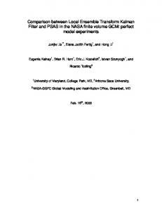
A set of 4.3 million temperature profiles and moored time series and 1.9 million salinity profiles spanning 1979–2003 was obtained from the World Ocean Database 2005 (Boyer et al., 2006). This profile data coverage is concentrated along shipping routes in the Northern Hemisphere and in some coastal regions. Temperature observations are also concentrated in the tropical Pacific while salinity observations are most prevalent in the North Atlantic and Indian Oceans. Salinity observation coverage increases rapidly throughout the experiment period due to the introduction of the Argo float network. This data underwent minor additional quality control and was then binned into daily 1◦ × 1◦ horizontal bins and linearly interpolated onto the model vertical levels (Fig. 1). We use validation data from two stations: the ALOHA station of the Hawaiian Ocean Time-series (Karl and Lukas, 1996) and Station S of the Bermuda Atlantic Time-series Study (Steinberg et al., 2001). The hydrography at Station S consists of a seasonally varying, up to 200 m-thick surface layer whose properties are controlled by local conditions superimposed on a roughly 200–400 m depth layer of www.nonlin-processes-geophys.net/20/1031/2013/


1033

relaxation to Levitus and Boyer (1994) climatological temperature and salinity at higher latitudes. We make no attempt ,-./-01230-" to model cryospheric or deep-water formation processes ex%#!!" 41567628" plicitly. A weak relaxation of the global temperature and salinity fields to climatological values with a 5 yr timescale is %!!!" included in order to reduce weak forecast bias in deep water $#!!" masses. Horizontal friction and diffusion coefficients have a constant value of 6 × 107 cm s−2 . Vertical friction and dif$!!!" fusion are Richardson number dependent with a maximum value of 3 cm s−2 . No explicit treatment of model bias was #!!" performed. Surface momentum and thermal forcing is provided by !" $'$'()" $'$'(*" $'$'(+" $'$'((" $'$'!!" $'$'!$" $'$'!%" $'$'!&" the NCEP/NCAR reanalysis of Kalnay et al. (1996) while Figure 1. Temperature and Salinity super-observation counts from Jan 1996 to Jan 2004. Eachsurface salinity is represented with a monthly climatology Fig. 1. Temperature and Salinity super-observation counts from Janfrom Levitus and Boyer (1994). Surface forcing fields are lindata represents a single day’sEach Argo and XBT profile data used for data assimilation, uarypoint 1996 to January 2004. data point represents a single day’s early interpolated from monthly averages. The Free Run was Argo and XBT profile data used for data assimilation, after horizonafter horizontal binning and interpolation to the model’s vertical levels. started from a state of rest with climatological temperature tal binning and interpolation to the model’s vertical levels. and salinity and run from years 1970 to 2004. Differences between the observations and the Free Run were calculated 2 quasi-uniform 18 ◦ C mode water (Joyce and Robins, 1996; for 1996–2003. These give a point of reference for the backPhillips and Joyce, 2007). The upper layer experiences shalground and analysis errors in the experiments. We assume Mean Obs Error 0ï500m low1.5depths, and reduced salinity in boreal summer the main source of forecast error in the ocean model comes Freewarming Run SODAcorresponding B and fall, and cooling, salinification, and deepfrom the surface forcing. For this study, we focus on wind SODA A 1winter and spring (annual ranges of temperening in late stress error, though we acknowledge additional sources of LETKF B 1 1 ature andLETKF salinity near-surface are 6 ◦ C and 0.15 psu). Susurface forcing error are important as well. In order to introA perimposed on this seasonal cycle temperature and salinity duce wind error with realistic spatial scales and seasonality RIP1 B0 of 0.5 the upper m undergo year-to-year fluctuations on the into the stress of the ith ensemble member, τ i , perturbations RIP1 200 B1 RIP1◦A1 order of 0.5 C and 0.05 psu, with cool temperatures in the were constructed by selecting stresses from the same month mid-1990s followed by1999a warming trend,2002 and substantially in different, randomly selected years from the entire NCEP 0 1996 1997 1998 2000 2001 2003 2004 reduced salinities for several Date years in the late 1990s. Below reanalysis period (a similar approach was used by Zhang et this layer the mode water thickness and salinity varies as a al., 2007). Thus τ i (tk ) is the weighted combination at time Figure 2. 12-month moving average of global temperature (ºC) RMSD O-B and O-A in the function of the intensity of winter storm activity, which was tk , 1 top 500 m for Standard-LETKF , and LETKF-RIP1. The background data reduced inFree-Run, the lateSODA, 1990s and early 2000s. For observed zonal velocities, we use the Acoustic τ i (tk ) = (1 − αw τ (tk ) + αw τ i (tk + m · 12 mo) (1) 23 Doppler Current Profile (ADCP) data that are part of the TAO/TRITON array located in the equatorial Pacific. The for some random integer n 6= 0. αw is the weighting that deavailable data during the experiment period from 1997–2003 termines the proportion of the historical perturbation used. are located on the equator at 165◦ E, 170◦ W, 140◦ W, and For the experiments reported here we used αw = 0.1. A simi110◦ W. Volume transports were estimated in the model as lar approach was used to generate the initial ensemble, using the integral of the velocity over a vertical cross section the historical Free Run data set as a basis with a weighting of each current, from the surface to 700 m depth for the coefficient equal to 0.5. Gulf Stream and Kuroshio Current, and from the surface to Our benchmark data assimilation experiment uses SODA 2400 m depth for the Agulhas Current. The model estimates (Carton et al., 2000a, b; Carton and Giese, 2008). SODA are compared to observations of volume transport as reported aggregates an extended (±45 day) window of observations, by Richardson (1985), Imawaki et al. (2001), and Bryden et with observations weighted by a Gaussian taper function al. (2005). While the major western boundary currents are centered at the analysis time. SODA specifies an empirical not well resolved in this model, the relative impacts of the anisotropic background error covariance that depends on latdifferent assimilation methods on the general circulation are itude, depth and dynamic height (see Carton et al., 2000a for noted. details). The vertical background error covariance is assumed Forecasts are made using an ocean model based on the to be large within the mixed layer, and decreases at deeper Geophysical Fluid Dynamics Laboratory (GFDL) Modular levels where the ocean is well mixed. Observation error is Ocean Model 2.2 (Pacanowski, 1996). The model resolution assumed to be uncorrelated white noise with an amplitude is 1◦ ×0.58◦ ×20 levels in the tropics, expanding to a uniform equal to 20 % of the zero lag model background error vari1◦ × 1◦ × 20 levels in mid-latitude for a total of 936 000 grid ance for temperature (T ), and 40 % for salinity (S), as specpoints. The basin domain extends from 62◦ S–62◦ N with a ified by Carton et al. (2000a). The salinity observation error &!!!"

1 2 3

Temperature RMSD (ºC)

4

5 6 7

www.nonlin-processes-geophys.net/20/1031/2013/

Nonlin. Processes Geophys., 20, 1031–1046, 2013

1034


values are effectively taken from the climatological T /S relationship to be consistent with the estimated temperature observation error values. SODA uses the two-stage Incremental Analysis Update (IAU) time filter of Bloom et al. (1996) to avoid generation of spurious gravity waves. After performing the analysis on the 5-day forecast, a 10-day forecast is performed in which the analysis increment is gradually introduced as a restoring force into the predictive equations for temperature and salinity. The second data assimilation algorithm we use is LETKF, a computationally efficient ensemble Kalman filter designed by Hunt et al. (2007) that uses the localization method of Ott et al. (2004) and a transformation between background and analysis ensemble perturbations similar to Bishop et al. (2001), Wang et al. (2003) and Ott et al. (2004). The algorithm uses an ensemble of numerical forecast model runs to estimate the background error covariance and assimilates observations at the time they occur rather than aggregating them at a fixed analysis time. A variable localization radius is used in LETKF to model the reduction of the radius of deformation with increasing latitude. LETKF’s estimates of observation error are taken from the SODA assimilation system. The separation of ensemble members in the state space should occur because of a combination of internal fluid instabilities and variations in surface forcing. The impacts of internal instabilities are greatly reduced because of our choice of non-eddy resolving resolution and associated physical parameterization errors. Additionally, limitations on the size of the ensemble further reduce the ensemble variance. We adjust for this missing error variance (1) in the model by adding perturbations to the wind field (as described above), and (2) in the data assimilation procedure through an adaptive error covariance inflation scheme developed by Miyoshi (2011). Miyoshi’s scheme has been applied to adjust inflation to automatically balance the background error with the estimated observation error. Occasionally, the ensemble spread becomes under-dispersive, meaning that the background error covariance estimate is small, while the mean state is “far” from the observations (with respect to the observation error). In these cases the inflation is automatically increased and the ensemble spread increases as a direct result. The ensemble spread continues to increase over multiple analysis cycles until the background error covariance is large enough that the observations begin to impact the analysis again. A parameter for adaptive inflation σb allows the inflation to be smoothed in time to achieve a larger effective sample size of observations. Miyoshi’s original method assumed that the spatial structure of the observing system remains constant in time. When applied to the oceanographic problem for which the observing system is constantly changing, Miyoshi’s approach has a tendency to increase background covariance in areas where observational coverage declines over time. Here, whenever observation coverage declines we relax inflation values back Nonlin. Processes Geophys., 20, 1031–1046, 2013

to the initial conditions in order to improve its performance for the sparse observation network. For the experiments described here, this relaxation was only applied in areas where the analysis spread for temperature was greater than 2 ◦ C. The final data assimilation algorithm is LETKF-RIP, utilizing the iterative dual-pass RIP procedure introduced by Kalnay and Yang (2010) and Yang et al. (2012a). RIP applies the weights computed for the end of the LETKF analysis cycle to the ensemble members at the beginning of the cycle, and the forecast and analysis steps are subsequently repeated. The result is a gradual correction to the background ensemble mean. Each repetition is based on the same set of observations, but initiates the dynamical model from different initial conditions. While this procedure could be repeated several times, it is only repeated once per analysis cycle in this study. Both the standard LETKF and LETKF-RIP use a 5 day analysis cycle so the background and analysis times correspond with SODA. Both ensemble methods use a 40member ensemble in all experiments reported here. LETKF implements localization by choosing observations around each model grid point subject to a cutoff radius. It then applies a Gaussian localization function to the estimated observation errors in this radius. The localization is parameterized by the σ -radius, which is the distance corresponding to one standard deviation of the Gaussian localization function. We report results from two parameter settings in LETKF, indicated by superscripts (if no superscript is used the statements apply to both). The first uses a horizontal σ -radius at the equator of about 300 km with a cutoff at 1100 km (denoted LETKF1 and LETKF-RIP1 ), and the second uses a σ -radius of 1100 km with a cutoff at about 4000 km (denoted LETKF2 and LETKF-RIP2 ). Both decrease linearly to an 80 km σ -radius with cutoff at 300 km at the ±60◦ latitude. The change in localization exhibited a nonlinear effect on the inflation values computed with the adaptive inflation algorithm, thus a smaller time-scaling factor σb = 0.0001 was used with the larger localization radius, versus σb = 0.001 for the smaller radius. In the vertical, a σ radius of about 80 m with a cutoff of 300 m was used. We will focus primarily on the results from LETKF1 and LETKFRIP1 , but include LETKF2 and LETKF-RIP2 for comparison.

3

Results

The following experiments are compared: A Free Run of the model with no data assimilation applied, SODA, LETKF1,2 and LETKF-RIP1,2 . We assess the performance of these data assimilation systems by first examining the consistency of statistical assumptions used in formulating the assimilation algorithms. In particular we focus on the root mean square deviation (RMSD) statistic of observation-minusbackground (O–B) and observation-minus-analysis (O–A) differences evaluated at the observation locations and times. www.nonlin-processes-geophys.net/20/1031/2013/

2

6 Each observations, they are directly comparable and show improvement by RIP. Because SODA Figure 1. Temperature and Salinity super-observation counts from Jan 1996 to Jan 2004.

3

7 uses a long window of observations, it is more appropriate to compare the background data point represents a single day’s Argo and XBT profile data used for data assimilation,

4

SODA-B versus RIP-B1 and the analysis SODA-A versus LETKF-A and RIP-A1. afterG. horizontal andThe interpolation to the model’stransform vertical levels. Kalman 8filter S. Pennybinning et al.: local ensemble 1035

0.7 0.6

Mean Obs Error 0ï500m Free Run RIP1 B0 SODA B

0.5

SODA A

1.5

1

0.5

Mean Obs Error 0ï500m Free Run SODA B SODA A

Salinity RMSD (psu)

Temperature RMSD (ºC)

2

LETKF1 B LETKF1 A RIP1 B0

5 6 7

0.4

RIP1 B1 RIP1 A1

1

LETKF A

0.3 0.2

1

RIP B1

0.1

RIP1 A1 0 1996

1

LETKF B

1997

1998

1999

2000 Date

2001

2002

2003

2004

0 1996

1997

1998

1999

2000 Date

2001

2002

2003

2004

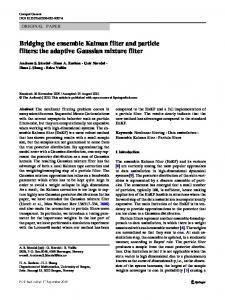
9 10in the Figure 3. 12-month moving average of global salinity (psu) RMSD O-B and O-A in the top Figure 2. 12-month moving average of global temperature (ºC) RMSD O-B and◦O-A

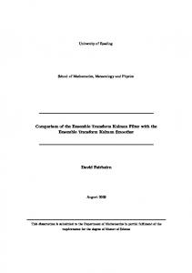
Fig. 2. A 12-month moving average of global temperature ( C) Fig. 3. A 12-month moving average of global salinity (psu) RMSD 1 RMSD O–B and O–A inStandard-LETKF the top 500 1m for Free Run, SODA, 11 data 500 m for Free-Run, SODA, and LETKF-RIP . The background 1 O–B and O–A in the Standard-LETKF top 500 m for1, Free Run, SODA, Standard-data are top 500 m for Free-Run, SODA, , and LETKF-RIP . The background 1 1 Standard-LETKF1 , and LETKF-RIP1 . The background data are LETKF , and LETKF-RIP . The background data are shown with 12 shown with dashed lines, and the analysis data with solid lines. In the legend, the suffix ‘B’ shown with dashed lines, and the analysis data with solid lines. In dashed lines, and the analysis data with solid lines. In the legend, 23 the legend, the suffix “B” signifies background, while “A” signifies13 signifies background, while ‘A’background, signifies analysis. For the RIPsignifies methods, ‘B0’ is the the suffix “B” signifies while “A” analysis. analysis. For the RIP methods, “B0” is the background of the iniFor the RIP methods, “B0” is the background of the initial iteration of the initial iteration of LETKF while ‘B1’ and ‘A1’ are the background and tial iteration of LETKF while “B1” and “A1” are the background14 background of LETKF while “B1” and “A1” are the background and analysis and analysis after the 1st iteration of RIP. The mean temperature15 analysis after1st the iteration 1st iterationof of RIP. mean salinity observation error in theerror top 500 m is after the RIP.The The mean salinity observation observation error in the top 500 m is shown with a dashed gray line. in the top 500 m is shown with a dashed gray line. Comparisons with a dashed gray line. As with the temperature RMSD in Figure 2, cases LETKF-B As cases LETKF-B and RIP-B0 have not used “future” observa-16 shown between the background SODA-B versus RIP-B1 and the analysis tions, they are directly comparable and show improvement by RIP. SODA-A versus LETKF-A and RIP-A1 show improvement by RIP. 24 Because SODA uses a long window of observations, it is more appropriate to compare the background SODA-B versus RIP-B1 and the analysis SODA-A versus LETKF-A and RIP-A1. 3.1 RMSD

For all methods other than SODA, the (O–B) RMSD are computed with observations that have not been used at all by the assimilation up to that time, thus these observations may be considered withheld for the purpose of comparison. The (O–A) RMSD at the corresponding time indicates the relative impact of the assimilation method. Adaptive inflation values are provided for additional perspective on the performance of the LETKF-based approaches. An increase in RMSD was noted as the ensemble size was reduced from 40 to 20 members, though results were qualitatively similar. To evaluate the analyses, we present comparisons to independent observations. We examine the relationship between observed and analysis temperature and salinity in the northern subtropical gyres through comparison to observed time series at Station S (30.6◦ N, 63.5◦ W) in the western subtropical North Atlantic and the Hawaii Ocean Time-series site (24.8◦ N, 158.0◦ W) near Oahu, Hawaii in the subtropical North Pacific. We examine zonal velocity anomalies using Tropical Atmosphere Ocean (TAO/TRITON) moorings in the equatorial Pacific (at 165◦ E, 170◦ W, 140◦ W and 110◦ W). Both observation and model data for the stations and moorings have been smoothed with a monthly average prior to this comparison. We also compare volume transport in selected major western boundary currents to observed values.


The aggregate RMSD for the final three years of the experiment period are shown for temperature (Table 1) and salinity (Table 2). Globally, LETKF and LETKF-RIP substantially improve the temperature fields over the SODA baseline. As can be seen in Fig. 2, the (O–B) temperature RMSD for LETKF1 and LETKF-RIP1 both fall below the SODA (O–B) baseline. The LETKF-RIP1 temperature (O–A) RMSD falls below the estimated observation error over a year before the standard LETKF analysis, while the SODA baseline never reaches this level. Throughout the experiment period, across all regions, the temperature fields for LETKF-RIP are as good or better than LETKF. LETKF-RIP takes advantage of the large estimated observation error (e.g. with a mean 0.67 psu in the top 500 m, as specified by SODA) and increases salinity RMSD in some regions to facilitate greater improvements in temperature. However, as shown in Fig. 3, by the end of the experiment period the salinity (O–B) RMSD for both LETKF1 and LETKF-RIP1 have fallen below the SODA baseline. The LETKF-RIP1 salinity (O–A) RMSD falls below the SODA baseline early in the experiment period, and this occurs over a year before the crossover by the standard LETKF1 analysis. Recall from Fig. 1 that there is an order of magnitude fewer salinity observations than temperature observations. For the salinity RMSD calculations, a small number of outlier observations from the Gulf Stream that caused a spike in RMSD (for both the Free Run and SODA) in the first two years of the experiment period were removed, though they Nonlin. Processes Geophys., 20, 1031–1046, 2013

1036


Table 1. Mean (observation-background) temperature RMS deviations (◦ C) for each method from January 2001–December 2003 listed globally, regionally, and by vertical level. Free Run

SODA

LETKF1

LETKF-RIP1

LETKF2

LETKF-RIP2

Global

2.03

1.23

1.03

1.01

1.23

1.17

N Pacific Eq Pacific S Pacific N Atlantic Eq Atlantic S Atlantic Indian

2.17 2.19 1.43 1.63 1.94 1.86 1.61

1.47 1.18 0.98 1.12 1.18 1.66 1.17

1.35 0.89 0.96 0.99 0.94 1.06 1.12

1.30 0.89 0.94 0.96 0.92 0.81 1.09

1.57 1.05 1.21 1.28 1.15 1.39 1.32

1.50 1.00 1.12 1.19 1.09 1.36 1.27

Global SFC Global 100 m Global 500 m

1.91 2.19 1.15

1.03 1.37 0.68

0.95 1.12 0.67

0.91 1.12 0.63

1.20 1.26 0.88

1.13 1.10 0.82

Table 2. Mean (observation-background) salinity RMS deviations (psu) or each method from January 2001–December 2003 listed globally, regionally, and by vertical level. Free Run

SODA

LETKF1

LETKF-RIP1

LETKF2

LETKF-RIP2

Global

0.34

0.26

0.26

0.26

0.31

0.31

N Pacific Eq Pacific S Pacific N Atlantic Eq Atlantic S Atlantic Indian

0.29 0.25 0.19 0.34 0.35 0.23 0.30

0.14 0.20 0.18 0.30 0.29 0.11 0.18

0.12 0.24 0.20 0.25 0.25 0.21 0.16

0.19 0.26 0.24 0.25 0.24 0.18 0.15

0.36 0.29 0.16 0.32 0.30 0.20 0.30

0.31 0.30 0.17 0.31 0.30 0.19 0.25

Global SFC Global 100 m Global 500 m

0.34 0.34 0.23

0.27 0.27 0.21

0.31 0.24 0.14

0.30 0.26 0.13

0.33 0.31 0.20

0.34 0.30 0.20

were used in the analyses. While the estimated observation error profiles were used from published results derived for the second half of the 20th century, the results in Fig. 3 indicate that a more sophisticated estimation of observation errors, varying not only by depth but also geographically and temporally, may further improve the analyses, particularly with the increase in quantity and accuracy of in situ salinity observations due to the Argo system. In Figs. 2 and 3 we show RMSD for both the background and analysis fields for SODA and LETKF1 . Because RIP is an iterative method, we show the background for the first (B0) and last (B1) iterations of LETKF-RIP1 , as well as the final analysis (A1). We note that the background fields for LETKF1 -B and RIP1 -B0 can be fairly compared since they do not use future observations, relative to the analysis time. Because SODA uses a long window of observations extending both into the past and future relative to the analysis time, it is more appropriate to compare the background field SODA-B with RIP1 -B1 and the analysis field SODAA with LETKF1 -A and RIP1 -A1. Figure 2 shows that the Nonlin. Processes Geophys., 20, 1031–1046, 2013

RIP-B0 RMSD with the temperature observations is significantly smaller than the corresponding LETKF-B during the spin up of the first four years, indicating that, in agreement with Kalnay and Yang (2010), RIP is particularly helpful during the spin up. During the last 3 yr included in Table 1, the advantage of RIP over the standard LETKF for temperatures is smaller but still positive. Both for salinity and for temperatures, the forecast from RIP-B1, started from the previous analysis updated with RIP is about as accurate as the analysis of the standard LETKF, and the LETKF-RIP analysis is significantly more accurate in RMSD, indicating that RIP succeeded in improving the quality of the previous analysis. We note that for reanalysis, the improvement of the previous analysis can be performed with the “no-cost smoother” of Kalnay et al., 2007; Yang et al., 2009, without incurring in the main computational cost of RIP, which is the re-forecasting of the ensemble.



1037

Table 3. Adaptive inflation values averaged per region. Values are reported at the end of the experiment period (approximately 1 January 2004). Larger adaptive inflation indicates model deficiencies in representing observed features. Adaptive inflation values are small in the southern oceans due to low data availability. Percent Inflation LETKF1

LETKF-RIP1

LETKF2

LETKF-RIP2

14.1 36.6 4.2 19.3 28.3 2.8 9.5 24.6 38.6

9.1 24.2 2.6 12.2 18.1 1.8 6.6 13.6 22.0

5.7 16.4 1.1 6.7 11.2 0.4 3.2 9.5 20.6

4.2 12.6 0.9 4.6 8.0 0.3 2.5 6.8 14.8

N Pacific Eq Pacific S Pacific N Atlantic Eq Atlantic S Atlantic Indian Gulf Stream Kuroshio

Table 4. Mean and standard deviation of volume transports for the Gulf Stream (off Cape Hatteras, 35◦ N, 0–700 m), Kuroshio Current (off Shikoku Island, ASUKA Line, 0–700 m), and Agulhas Current (off Port Edward, 33◦ S, 0–2400 m) from 1997 to 2003. Mean Volume Transport in Sverdrups (Sv), and (standard deviation)

Gulf Stream Kuroshio Agulhas

Free Run

SODA

LETKF1 LETKFRIP1

LETKF2 LETKFRIP2

Observed

28.8 (1.7) 34.1 (1.9) 77.5 (22.7)

46.2 (21.1) 56.7 (16.7) 78.3 (23.3)

38.0 (7.4) 44.7 (11.0) 76.8 (22.7)

32.4 (2.0) 40.1 (3.0) 77.4 (22.7)

60* (55) 42** (1.3) 69.7*** (21.5)

41.5 (10.1) 46.5 (14.0) 76.4 (22.6)

34.0 (2.5) 42.1 (3.9) 77.5 (22.8)

* Richardson (1985); ** Imawaki et al. (2001); *** Bryden et al. (2005).

3.2

Adaptive inflation parameter by region

As discussed in Sect. 2, inflation is needed to artificially enhance growth of the ensemble spread due to the viscous nature of the 1 × 1◦ model grid resolution. The adaptive inflation procedure increases inflation for areas in which the model error is estimated to be too small based on comparison with local observations. In a well-observed region, smaller values of inflation indicate a more appropriate ensemble in approximating the background covariance given the observation errors, as described by the diagnostic equations of Desroziers et al. (2005) and Li et al. (2009). Average inflation values for LETKF and LETKF-RIP are given for each region in Table 3. In general, the inflation values are larger in the western boundary currents and in the equatorial regions of the Atlantic and Pacific oceans. However, because the adaptive inflation calculation can only be performed when observations are present, it is noted that adaptive inflation is roughly proportional to the number of observations available in each region over the duration of the experiment period. The adaptive inflation values for LETKF-RIP are less than that for LETKF. This indicates a reduced need for inflation with the RIP method. Both inflation and RIP provide a means www.nonlin-processes-geophys.net/20/1031/2013/

to increase the effect of specific observations on the analysis. While adaptive inflation builds a long-term “memory” of geographic areas where the model consistently disagrees with observations, RIP reforms the initial ensemble to immediately increase the impact of observations in areas where the model uncertainty is largest. 3.3 Comparisons with independent observations at station S and Aloha Next we present comparisons of the analyses against independent time series of temperature and salinity at two subtropical locations in the North Atlantic and North Pacific. Our comparison of the Free Run and assimilation experiments at Station S shows that the Free Run has a difficult time representing the mean vertical structure of temperature (Fig. 4) or salinity (Fig. 5). In particular, it is over 3 ◦ C too warm in the upper 200 m and 3 ◦ C too cold in the depth range 200–400 m, implying that it is too strongly stratified, and is also too fresh by up to 0.5 psu. All of the assimilation methods reduce this mean stratification error. After assimilation the salinity analyses are no longer uniformly fresh, but develop a pattern of salty and Nonlin. Processes Geophys., 20, 1031–1046, 2013

2

background SODA-B versus RIP-B1 and the analysis SODA-A versus LETKF-A and RIP-A1

3

also show improvement by RIP.

1038


Free Run

SODA

LETKF1

LETKF-RIP1

LETKF2

LETKF-RIP2

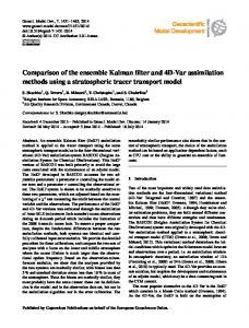
4 Fig. 4. Temperature analysis minus bottle temperature measurement (◦ C) at Station S (Bermuda; (30.55–63.5)) from January 1997 to December 2003 for the top 500 m. From top to bottom: Free Run, SODA, LETKF1 , LETKF-RIP1 , LETKF2 , and LETKF-RIP2 . Red shows that 4. Temperature temperature measurement at Station the analysis 5 is tooFigure warm, and blue too cold, analysis comparedminus to the bottle independent observation. White gaps(ºC) indicate missingS observation data. 6

(Bermuda; (30.55,-63.5)) from Jan. 1997 to Dec. 2003 for the top 500 m. From top to bottom:

7

1 1 2 2 Free Run, Free SODA, Run LETKF , LETKF-RIP , LETKF , and LETKF-RIP . Red shows that the

8

analysis is too warm, and blue too cold, compared to the independent observation. White gaps

9

indicate missing observation data.

SODA

LETKF1

LETKF-RIP1

25 LETKF2

LETKF-RIP2

1 analysis minus bottle measurement (psu) at Station S (Bermuda; (30.55–63.5)) from January 1997 to December 2003 for the Fig. 5. Salinity top 500 m. From top to bottom: Free Run, SODA, LETKF1 , LETKF-RIP1 , LETKF2 , and LETKF-RIP2 . 2

Figure 5. Salinity analysis minus bottle measurement (psu) at Station S (Bermuda; (30.55,-

3

63.5)) from Jan. 1997 to Dec. 2003 for the top 500 m. From top to bottom: Free Run, SODA,

1 1 2 4 LETKF , LETKF-RIP , LETKF , and LETKF-RIP2. Nonlin. Processes Geophys., 20, 1031–1046, 2013

5



1039

Free Run

SODA

LETKF1

LETKF-RIP1

LETKF2

LETKF-RIP2

Fig. 6. Temperature analysis minus bottle measurement (◦ C) at Aloha Station (24.75–158.0) from January 1997 to December 2003 for the 1 top 500 m. From top to bottom: Free Run, SODA, LETKF1 , LETKF-RIP1 , LETKF2 , and LETKF-RIP2 .

2

Figure 6. Temperature analysis minus bottle measurement (ºC) at Aloha Station (24.75,-

3

158.0) from Jan. 1997 to Dec. 2003 for the top 500 m. From top to bottom: Free Run, SODA,

4

LETKF1, LETKF-RIP1, LETKF2, and LETKF-RIP2. Free Run

SODA

LETKF1

LETKF-RIP1

LETKF2

LETKF-RIP2

27

1 analysis minus bottle measurement (psu) at Aloha Station (24.75–158.0) from Januar 1997 to December 2003 for the top Fig. 7. Salinity 500 m. From top to bottom: Free Run, SODA, LETKF1 , LETKF-RIP1 , LETKF2 , LETKF-RIP2 . 2

Figure 7. Salinity analysis minus bottle measurement (psu) at Aloha Station (24.75,-158.0)

3

from Jan. 1997 to Dec. 2003 for the top 500 m. From top to bottom: Free Run, SODA,

4 LETKF1, LETKF-RIP1, LETKF2, LETKF-RIP2. www.nonlin-processes-geophys.net/20/1031/2013/ 5


1040

S. G. Penny et al.: The local ensemble transform Kalman filter Station S Mean Salinity RMSD

0

100

100

Depth (m)

Depth (m)

Station S Mean Temperature RMSD

0

200 300

1

300 400

400 500 0

200

0.5

1

1.5

RMSD (ºC)

2

500 0

2.5

0

100

100

200 300 400

2

500 0

0.4

0.6

RMSD (psu)

0.8

1

ALOHA Station Mean Salinity RMSD

0

Depth (m)

Depth (m)

ALOHA Station Mean Temperature RMSD

0.2

200 300 400

0.5

1

1.5

RMSD (ºC)

2

2.5

500 0

0.2

0.4

0.6

RMSD (psu)

0.8

1

3 and Figure 8. Mean temperature and salinitybottle (analysis minus independent measurements) Fig. 8. Mean temperature salinity (analysis minus independent measurements) RMSD atbottle Station S and Aloha Station corresponding to Figs. 4–7. Results are shown for the Free Run (solid grey), SODA (green), LETKF1 (blue), and LETKF-RIP1 (purple), with the observation RMSD(dashed at Station S and Aloha Station corresponding to Figures 4-7. Results are shown for the error profile shown for4reference grey). 5

Free Run (solid grey), SODA (green), LETKF1 (blue), and LETKF-RIP1 (purple), with the

1 1 2 fresh anomalies that6 areobservation trapped near surface. LETKF-RIP error the profile shown LETKF for reference (dashed grey). over LETKF , but worsened by LETKF-RIP 2 seems to still be adjusting mean temperatures throughout over LETKF . the early years of the experiment and thus are still too cold At Station Aloha in the subtropical North Pacific, the upbetween 200–400 m,7 whereas in SODA they are too warm. per 400 m contains a warm salty layer at 0–200 m with temThis corrective warming occurs more gradually in LETKF peratures of 18◦ −23 ◦ C and salinities 34.9–35.2 psu, drop8 but is accelerated by LETKF-RIP. All analyses show erroping to 14 ◦ C and 34.1 psu by 400 m depth. The seasonal cyneously warm surface temperatures in winter. In most cases, cle at this location is relatively weak. Salinity in this upper LETKF-RIP reduces the error compared to LETKF, though layer typically exhibits a subsurface maximum reflecting its there is a slight increase in errors in the summer of 2000 by origin through subduction along the subtropical front. DurLETKF-RIP1 . Both methods seem to improve the warm wining our period of interest conditions were anomalously dry, ter anomalies versus SODA. While LETKF1 does this by leading to heavier than normal surface water and more extenallowing freshwater anomalies at the surface, the effect is sive exchanges throughout the upper 200 m (Lukas, 2001). mitigated by LETKF-RIP. The summer of 2002 is unusual The Free Run at this location has temperatures that are too in all three experiments in showing anomalously cool wacool by several degrees and salinities that are too fresh by ter throughout the upper 400 m relative to observed condi0.3 psu (more consistent with salinities earlier in the decade). tions, which were themselves anomalously cool with deep Again, the analyses all show a reduction in the temperature penetration of the winter mixed layer. During the anoma(Fig. 6) and salinity deviations (Fig. 7) from observations. In 29 lous conditions of summer 2002, all three assimilation exall experiments, temperatures remain too cold in the upper 2 periments exhibit elevated surface salinities, while SODA 300 m. SODA, LETKF and LETKF-RIP2 remain too fresh has anomalously low salinity below 200 m. In some cases, in the upper 200–300 m. This fresh bias is corrected starting LETKF-RIP reduces the salinity errors exhibited by LETKF, in 2000 by LETKF1 , and to a greater degree LETKF-RIP1 , e.g. below 200 m in 1997–1998, throughout 0–400 m from with some slight overshooting. However, as in the case for 1999–2001. The anomalously high surface salinities in sumStation S, LETKF1 and LETKF-RIP1 analysis errors have mer 2002 are reduced by LETKF-RIP, though this correction more variation in time than the other methods. This is exappears to have caused fresh anomalies in the subsequent pected, as SODA uses a rolling window of observations that winter months for LETKF-RIP1 . In other cases, LETKF-RIP extends well beyond the analysis cycle and is implemented increases the salinity errors, e.g. the autumn months of 1997, via a forcing term (via IAU). Both LETKF2 and LETKF2000, 2002 and 2003. In winter 2002, errors are improved by RIP2 exhibit a more gradual adjustment due to the larger




1041

Observed

Free Run

SODA

LETKF1

LETKF-RIP1

LETKF2

LETKF-RIP2

1 averaged zonal velocity at (0◦ N, 165◦ E) for observations and analyses from January 1997 to December 2003 from 30 to Fig. 9. Monthly 270 m, with time mean removed. From top to bottom: Observed ADCP data, Free Run, SODA, LETKF1 , LETKF-RIP1 , LETKF2 , LETKF2 Figure 9. Monthly averaged zonal velocity at (0N, 165E) for observations and analyses from RIP2 . 3 Jan. 1997 to Dec. 2003 from 30 to 270 m, with time mean removed. From top to bottom: spatial localization and the more gradual time smoothing pamodel, all of the methods underestimate the intensity of the 1 2 4 forObserved ADCP data, Free Run, SODA, LETKF1observed , LETKF-RIP LETKF2Therefore, , LETKF-RIP . rameter used adaptive inflation. zonal ,velocity. we remove the time mean The time mean (A–O) RMSD are shown for the Free Run, of each field and examine the monthly mean observed and SODA, LETKF1 and LETKF-RIP1 , relative to the observaanalyzed zonal velocity anomalies. Due to the large obsertion error profile. At both stations, the mean temperature devation window used in its analysis cycle, SODA appears viations are reduced by all methods. For Station S, LETKFto average out much of the small-scale temporal variability. RIP1 gives the greatest improvement in the top 200 m, folIn contrast, the ensemble methods exhibit some features on lowed by LETKF1 and SODA. From 200 to 500 m SODA smaller temporal scales. give results closest to the observation error profile, followed At 165◦ E (Fig. 8), a strong positive anomaly occurs by LETKF-RIP1 and LETKF1 . LETKF-RIP1 and LETKF1 throughout much of 1998. This feature is captured in part by have larger salinity RMSD at Station S in the upper 270 m, all methods, but is strongest in LETKF2 and LETKF-RIP2 . A negative anomaly that exists weakly in the Free Run in early closer to the estimated observation error profile. While be2002 appears to be represented most accurately by LETKFlow 270 m, the RMSD is smallest with LETKF-RIP1 , then LETKF1 and SODA, the latter being closest to the estimated RIP1,2 . At 170◦ W (Fig. 9), the overall anomaly pattern that alternates between positive and negative appears to be observation error. At Aloha Station all methods give approximately equal RMSD, though LETKF-RIP1 is lower overall. represented most accurately by LETKF-RIP1 . The positive 30 2 and LETKFThe salinity RMSD at this station are lowest with SODA and anomaly of 1998 is best captured by LETKF RIP2 . At 140◦ W (Fig. 10), SODA best represents the strong closest to the estimated observation error with LETKF-RIP1 . positive anomalies, though all of the methods strengthen the 3.4 Comparison with independent observations signal compared to the Free Run. LETKF2 has a slight repof velocity resentation of the positive anomaly that occurs just after the strong negative anomaly at the start of 1998. While absent We next compare to the observed zonal velocity profiles in in the SODA result, some of the weaker signals throughout the equatorial Pacific. Due to the coarse resolution of the



1042


Observed

Free Run

SODA

LETKF1

LETKF-RIP1

LETKF2

LETKF-RIP2

Fig. 10. Monthly averaged zonal velocity at (0◦ N, 170◦ W) for observations and analyses from January 1997 to December 2003 from 1 30 to 270 m, with time mean removed. From top to bottom: observed ADCP data, Free Run, SODA, LETKF1 , LETKF-RIP1 , LETKF2 , LETKF-RIP22 . Figure 10. Monthly averaged zonal velocity at (0N, 170W) for observations and analyses

3 from Jan. 1997 to Dec. 2003 from 30 to 270 m, with time mean removed. From top to bottom: level and heat content. The transports in the Gulf Stream and the experiment seem to be present in LETKF1 and LETKF1 are increased toward2.the observed values. RIP2 . At 110 (Fig. 11),ADCP the analysis signal corresponding 4 ◦W Observed data, Free Run, SODA, LETKF1Kuroshio , LETKF-RIP , LETKF2slightly , LETKF-RIP 1 The transport in the Agulhas is relatively unchanged commost to the observed signal appears to come from LETKF . pared to the observed and modeled variance. All of the methods have a negative anomaly at the surface that conflict with the observed signal, though SODA has the largest error. A number of observed positive anomalies are 4 Conclusions present in the Free Run and strengthened in the LETKF1 1 and LETKF-RIP analyses. SODA generates some spurious We have performed a comparison of the Local Ensemble positive anomalies throughout 2001 and 2002. LETKF1 and Transform Kalman Filter (LETKF) to a benchmark ocean asLETKF-RIP1 best capture the negative anomy at the end of similation system (SODA) using an identical global ocean 2002, while none of the methods adequately capture the almodel with identical observed temperature and salinity proternating positive and negative anomalies of 2003. file data set, initial conditions, and surface forcing. Two versions of LETKF were examined: the standard LETKF and 3.5 Volume transport in select western boundary LETKF-RIP, which uses the “running-in-place” (RIP) algocurrents rithm of Kalnay and Yang (2010) and Yang et al. (2012a,b). The results from each experiment were evaluated through Volume transports for the Gulf Stream, Kuroshio Current, 31 two approaches: (1) through comparison of the background and Agulhas Current are given in Table 4 as compared with field to the (not yet assimilated) observations of temperapublished observed values. All assimilation methods imture and salinity, and (2) through comparisons of the analproved transport toward observed levels when compared to yses to independent observations that included ocean station the Free Run baseline. The increased transport in the matime series in the North Pacific and North Atlantic subtropijor ocean basins, combined with a geostrophic balance as cal gyres, ADCP zonal velocity in the equatorial Pacific, and imposed by the model, implies an increased density gradimajor western boundary transports. ent within the basin and thus an increased anomaly of sea Nonlin. Processes Geophys., 20, 1031–1046, 2013



1043

Observed

Free Run

SODA

LETKF1

LETKF-RIP1

LETKF2

LETKF-RIP2

1 averaged zonal velocity at (0◦ N, 140◦ W) for observations and analyses from January 1997 to December 2003 from Fig. 11. Monthly 30 to 270 m, with time mean removed. From top to bottom: observed ADCP data, Free Run, SODA, LETKF1 , LETKF-RIP1 , LETKF2 , Figure 11. Monthly averaged zonal velocity at (0N, 140W) for observations and analyses LETKF-RIP22 . 3 from Jan. 1997 to Dec. 2003 from 30 to 270 m, with time mean removed. From top to bottom: Examination of temperature observation-minussubstantial biases of both temperature and salinity. These bi1 1 2 Observed shows ADCP data, Free Run, SODA, LETKFases , LETKF-RIP , LETKF LETKF-RIP2methods. . background 4 differences a reduction of errors were reduced by all, assimilation At Aloha a compared to the SODA baseline when using both LETKF cool, fresh bias remains in the high salinity upper 200 m, and LETKF-RIP, with the latter showing the greatest impact while a slight warm bias with elevated salinity is generally especially during the first four years of spin up. Globally, present between 200–400 m. The time series at Aloha is notemperature observation-minus-background differences table for cool anomalies in 1998–1999, and for a period of were smaller for LETKF-RIP than for SODA while salinity enhanced salinity beginning in the late 1990s where salinremained relatively unchanged compared the magnitude of ities exceeded 35.1 psu. These anomalies were weak in the estimated observation errors. We emphasize that both the Free Run, but better reproduced in the assimilation experiLETKF and LETKF-RIP background fields, which did not ments. During the years of the high salinity anomaly SODA use future data relative to the analysis time and whose RMS has salinity errors below 0.4 psu. LETKF-RIP shows much deviations were computed against observations that were not smaller average salinity errors, but with stronger year-to-year yet assimilated, achieved lower RMSD than SODA which variability. did use future data. Regionally the same results were found At Station S the Free Run also exhibits large biases in temfor temperature, while salinity RMSD was typically smaller perature and salinity, with too warm temperatures in the upin well-observed areas and larger in poorly observed areas. per 200 m, too cold temperatures below, and 32too fresh everyThe reduction in background error implies a corresponding where. The three assimilation experiments all reduced these improvement of the prior analysis, however additional mean biases, though all three have a residual seasonal bias comparisons were made to independent observed data to in near-surface temperature (too warm in winter, too cold assess the analyses themselves. in summer) likely reflecting errors in surface heating. AsIn order to evaluate the performance of the experiments similation substantially reduced the fresh bias in all three in the subtropical gyres the analyses were compared against experiments. Both LETKF1 and LETKF-RIP1 exhibit more withheld ocean station time series at Aloha near Hawaii, and year-to-year variations in salinity error than SODA, while Station S near Bermuda. At these stations the Free Run has LETKF2 and LETKF-RIP2 exhibit somewhat less, indicating



1044


Observed

Free Run

SODA

LETKF1

LETKF-RIP1

LETKF2

LETKF-RIP2

1 Fig. 12. Monthly averaged zonal velocity at (0◦ N, 110◦ W) for observations and analyses from January 1997 to December 2003 from 30 to 270 m, with time mean removed. From top to bottom: observed ADCP data, Free Run, SODA, LETKF1 , LETKF-RIP1 , LETKF2 , LETKF-RIP22 . Figure 12. Monthly averaged zonal velocity at (0N, 110W) for observations and analyses 3 from Jan. 1997 to Dec. 2003 from 30 to 270 m, with time mean removed. From top to bottom: that the localization and inflation parameters can be tuned This LETKF system has been implemented at the National 1 2 4 rapidly Observed ADCPadjusts data, Free Run, SODA, LETKF1Centers , LETKF-RIP , LETKF2, LETKF-RIP to control how LETKF to available observafor Environmental Prediction .(NCEP) with the options. erational GFDL ocean model that is currently used by the Due to model resolution, the modeled zonal velocities at Global Ocean Data Assimilation System (GODAS), which the equator5were much weaker than observed. After removis a component of NCEP’s Coupled Forecast System (CFS). ing the time mean, comparisons to observed zonal velocities The LETKF algorithm will form the ensemble component in the equatorial Pacific still showed that many of the obof a hybrid ocean data assimilation system that is being deserved anomalies were either weak or not present in the Free veloped for use by NCEP. For the purpose of reanalysis, the Run. However, all of the assimilation methods improved the practically cost-free RIP step applying the LETKF weights pattern of anomalies, typically strengthening both the posiobtained at the end of each assimilation window to the entive and negative anomalies to better coincide with the obsemble at the beginning of the window may be used to imserved anomalies. prove the previous analysis and thus smooth the overall time This study has a number of limitations. The model, choevolution of the analyzed fields. In addition, this LETKF sen for its computational efficiency, does not resolve the system will be used to assimilate the ocean component of ocean mesoscale. The lack of mesoscale processes likely a strongly coupled data assimilation system that is currently contributes to the presence of large mean biases. The exbeing designed by the University of Maryland for India’s Na33 periments are limited to a seven-year period, which is insuftional Monsoon Mission. ficient to examine the impact of differences in assimilation on longer time-scale processes. While we made great efforts Acknowledgements. We gratefully acknowledge: the Laboratory to make a fair comparison between methods, differences in for Microbial Oceanography within the School of Ocean and Earth practical implementation made a truly exact comparison imScience and Technology at the University of Hawaii at Manoa possible. which maintains the Aloha time series, the Bermuda Biological Station for Research which maintains Station S, and the National Oceanographic Data Center which maintains global hydrographic



S. G. Penny et al.: The local ensemble transform Kalman filter data. J. A. Carton, G. A. Chepurin and S. G. Penny acknowledge support by the National Science Foundation (OCE0752209). E. Kalnay acknowledges support from the National Aeronautical and Space Administration (NNX08AD40G, NNX11AH39G, NNX11AL25G) and India’s National Monsoon Mission. K. Ide and T. Miyoshi acknowledge support from the National Oceanic and Atmospheric Administration (NA09OAR4310178) and the Office of Naval Research (N000141010557, N000140910418). Edited by: G. Desroziers Reviewed by: two anonymous referees

References Bishop, C. H., Etherton, B. J., and Majumdar, S. J.: Adaptive Sampling with Ensemble Transform Kalman Filter, Part I: Theoretical Aspects, Mon. Weather Rev., 129, 420–436, 2001. Bloom, S. C., Takacs, L. L., da Silva, A. M., and Ledvina, D.: Data Assimilation using Incremental Analysis Updates, Mon. Weather Rev., 124, 1256–1271, 1996. Boyer, T. P., Antonov, J. I., Garcia, H., Johnson, D. R., Locarnini, R. A., Mishonov, A. V., Pitcher, T., Baranova, O. K., and Smolyar, I.: World Ocean Database 2005, Chapter 1: Introduction, NOAA Atlas NESDIS 60, Ed. S. Levitus, US Government Printing Office, Washington, DC, 182 pp., DVD, 2006. Brusdal, K., Brankart, J. M., Halberstadt, G., Evensen, G., Brasseur, P., Van Leeuwen, P. J., Dombrowsky, E., and Verron, J.: A demonstration of ensemble based assimilation methods with a layered OGCM from the perspective of operational ocean forecasting systems, J. Mar. Syst/, 40–41, 253–289, 2003. Bryden, H. L., Beal, L. M., and Duncan, L. M.: Structure and Transport of the Agulhas Current and Its Temporal Variability, J. Oceanogr., 61, 479–492, 2005. Carton, J. A. and Giese, B. S.: A Reanalysis of Ocean Climate Using Simple Ocean Data Assimilation (SODA), Mon. Weather Rev., 136, 2999–3016, 2008. Carton, J. A. and Santorelli, A.: Global Decadal Upper-Ocean Heat Content as Viewed in Nine Analyses, J. Climate, 21, 6015–6035, 2008. Carton, J. A., Chepurin, G., Cao, X., and Giese, B.: A Simple Ocean Data Assimilation Analysis of the Global Upper Ocean 1950–95 Part I: Methodology, J. Phys. Oceanogr., 30, 294–309, 2000a. Carton, J. A., Chepurin, G., Cao, X., and Giese, B.: A Simple Ocean Data Assimilation Analysis of the Global Upper Ocean 1950–95 Part II: Results, J. Phys. Oceanogr., 30, 311–326, 2000b. Cummings, J., Bertino, L., Brasseur, P., Fukumori, I., Kamachi, M., Martin, M. J., Mogensen, K., Oke, P., Testut, C. E., Verron, J., and Weaver, A.: Ocean data assimilation systems for GODAE, Oceanography, 22, 96–109, 2009. Desroziers G., Berre, L., Chapnik, B., and Poli, P.: Diagnosis of observation, background and analysis error statistics in observation space, Q. J. R. Meteorol. Soc., 131, 3385–3396, 2005. Evensen, G.: Sequential data assimilation with a nonlinear quasigeostrophic model using Monte Carlo methods to forecast error statistics, J. Geophys. Res., 99, 10143–10162, 1994. Fukumori, I., Benveniste, J., Wunsch, C., and Haidovogel, D. B.: Assimilation of sea surface topography into an ocean circulation model using a steady-state smoother, J. Phys. Oceanogr., 23, 1831–1855, 1993.


1045

Hunt, B. R., Kostelich, E. J., and Szunyogh, I.: Efficient Data Assimilation for Spatiotemporal Chaos: A Local Ensemble Transform Kalman Filter, Phys. D, 230, 112–126, 2007. Imawaki, S., Uchida, H., Ichikawa, H., Fukasawa, M., Umatani, S., and the ASUKA Group: Satellite altimeter monitoring the Kuroshio transport south of Japan, Geophys. Res. Lett., 28, 17– 20, 2001. Joyce, M. T. and Robins, P.: The Long-Term Hydrographic Record at Bermuda. J. Climate, 9, 3121–3131, 1996. Kalnay, E.: Atmospheric Modeling, Data Assimilation and Predictability, Cambridge University Press, Chapter 5, 2003. Kalnay, E. and Yang, S.-C.: Accelerating the spin-up of Ensemble Kalman Filtering, Q. J. R. Meteor. Soc., 136, 1644–1651, 2010. Kalnay, E., Kanamitsu, M., Kistler, R., Collins, W., Deaven, D., Gandin, L., Iredell, M., Saha, S., White, G., Woollen, J., Zhu, Y., Chelliah, M., Ebisuzaki, W., Higgins, W., Janowiak, J., Mo, K. C., Ropelewski, C., Wang, J., Leetmaa, A., Reynolds, R., Jenne, R., and Joseph, D.: The NCEP/NCAR 40-year reanalysis project, Bull. Am. Meteorol. Soc., 77, 437–471, 1996. Kalnay, E., Li, H., Miyoshi, T., Yang, S.-C., and Ballabrera-Poy J.: 4-D-Var or ensemble Kalman filter?, Tellus A, 59, 758–773, 2007. Karl, D. M. and Lukas, R.: The Hawaiian Ocean Time-series program: Background, rationale and field implementation, Deep Sea Res. II, 43, 129–156, 1996. Keppenne, C. L., Rienecker, M. M., Jacob, J. P., and Kovach, R.: Error covariance modeling in the GMAO ocean ensemble Kalman filter, Mon. Weather Rev., 136, 2964–2982, 2008. Levitus, S. and Boyer, T.: World Ocean Atlas 1994, vol. 4, Temperature, NOAA Atlas NESDIS, 129 pp., NOAA, Silver Spring, MD, 1994. Li, H., Kalnay, E., and Miyoshi, T.: Simultaneous estimation of covariance inflation and observation errors within an ensemble Kalman filter, Q. J. R. Meteor. Soc., 135, 523–533, 2009. Lukas, R.: Freshening of the upper thermocline in the North Pacific subtropical gyre associated with decadal changes of rainfall, Geophys. Res. Lett., 28, 3485–3488, 2001. Miyoshi, T.: The Gaussian Approach to Adaptive Covariance Inflation and its Implementation with the Local Ensemble Transform Kalman Filter, Mon. Weather Rev., 139, 1519–1535, 2011. Ott, E., Hunt, B. R., Szunyogh, I., Zimin, A. V., Kostelich, E. J., Corazza, M., Kalnay, E., Patil, D. J., and Yorke, J. A.: A Local Ensemble Kalman Filter for Atmospheric Data Assimilation, Tellus, 56A, 415–428, 2004. Pacanowski, R. C.: MOM2 Version 2.0 (Beta) Documentation, Users Guide and Reference Manual, GFDL Ocean Technical Report 3.2, Geophysical Fluid Dynamics Laboratory/NOAA, Princeton, N.J., 08542, 1996. Penny, S. G.: Data Assimilation of the Global Ocean using the 4D Local Ensemble Transform Kalman Filter and the Modular Ocean Model. Doctoral Dissertation, Applied Mathematics and Scientific Computation, University of Maryland, College Park, MD, 2011. Pham, D. T., Verron, J., and Roubaud, M. C.: A singular evolutive extended Kalman filter for data assimilation in oceanography, J. Mar. Syst., 16, 323–340, 1998. Phillips, H. E. and Joyce, M. T.: Bermuda’s Tale of Two Time Series: Hydrostation S and BATS, J. Phys. Oceanogr., 37, 554–571, 2007.


1046


Richardson, P. L.: Average velocity and transport of the Gulf Stream near 55W, J. Mar. Res., 43, 83–111, 1985. Steinberg, D. K., Carlson, C. A., Bates, N. R., Johnson, R. J., Michaels, A. F., and Knap, A. H.: Overview of the US JGOFS Bermuda Atlantic Time-series Study (BATS): a decade-scale look at ocean biology and biogeochemistry, Deep Sea Res. II, 48, 1405–1447, 2001. Wan, L., Zhu, J., Bertino, L., and Wang, H.: Initial ensemble generation and validation for ocean data assimilation using HYCOM in the Pacific, Ocean Dynam., 58, 81–99, doi:10.1007/s10236008-0133-x, 2008. Wan, L., Bertino, L., and Zhu, J.: Assimilating altimetry data into a HYCOM model of the Pacific: Ensemble Optimal Interpolation versus Ensemble Kalman Filter, J. Atmos. Ocean. Technol., 27, 753–765, 2010. Wang, X. and Bishop, C. H.: A Comparison of Breeding and Ensemble Transform Kalman Filter Ensemble Forecast Schemes, J. Atmos. Sci., 60, 1140–1158, 2003. Xue, Y., Balmaseda, M. A., Boyer, T., Ferry, N., Good, S., Ishikawa, I., Kumar, A., Rienecker, M., Rosati, A. J., and Yin, Y.: A Comparative Analysis of Upper-Ocean Heat Content Variability from an Ensemble of Operational Ocean Reanalyses, J. Climate, 25, 6905–6929, doi:10.1175/JCLI-D-11-00542.1, 2012.


Yang, S.-C., Lin, K.-J., Miyoshi, T., and Kalnay, E.: Improving the spin-up of regional EnKF for typhoon assimilation and forecasting with Typhoon Sinlaku (2008), Tellus A, 65, 20804, doi:10.3402/tellusa.v65i0.20804, 2013. Yang, S.-C., Corazza, M., Carrassi, A., Kalnay, E., and Miyoshi, T.: Comparison of ensemble-based and variational-based data assimilation schemes in a quasi-geostrophic model, Mon. Weather Rev., 137, 693–709, 2009. Yang, S.-C., Kalnay, E., and Hunt, B. R.: Handling nonlinearity in Ensemble Kalman Filter: Experiments with the threevariable Lorenz model, Mon. Weather Rev., 240, 2628–2646, doi:10.1175/MWR-D-11-00313.1, 2012a. Yang, S.-C., Kalnay, E., and Miyoshi, T.: Improving EnKF spinup for typhoon assimilation and prediction, Weather Forecast., 27, 878–897, 2012b. Zhang, S. and Rosati, A.: An Inflated Ensemble Filter for Ocean Data Assimilation with a Biased Coupled GCM, Mon. Weather Rev., 138, 3905–3931, 2010. Zhang, S., Harrison, M. J., Rosati, A., and Wittenberg, A.: System design and evaluation of coupled ensemble data assimilation for global oceanic climate studies, Mon. Weather Rev., 135, 3541– 3564, 2007.
