Abstract- This paper studies a M/G/1 queueing system with vacations, in which the sojourn time of the server at the queue is controlled by a timer. We consider ...
IEEE TRANSACTIONS ON COMMUNICATIONS, VOL. 42, NO. 21314, FEBRUARYIMARCHIAPRIL 1994
1846
The
Queueing System with Vacations and Timer-Controlled Service Jhitti Chiarawongse, Mandyam M. Srinivasan and Toby J. Teorey
Abstract- This paper studies a M/G/1 queueing system with vacations, in which the sojourn time of the server at the queue is controlled by a timer. We consider three policies for setting the timer value: time-limited (TL), cycletime-limited (CL) and cycle-time-limited with accumulated lateness (CLL). When the server arrives at the queue, the timer is set to a certain value depending on the policy employed. The server serves the waiting customers until either the system becomes empty, or the timer expires, whichever occurs first. In the latter case, the server completes the service on the customer being served, then takes a vacation. Customers are not served during the vacation. If the system is empty upon the server's return from a vacation, another vacation begins immediately. Such a queueing system finds applications in the performance analysis of local area network protocols such as the IEEE 802.4 (token bus) and the Fiber Distributed Data Interface (FDDI), in which the vacation would correspond to the time the token is away at other stations. Using the matrix-analytic approach, we compute the probability distribution of the number of customers in the system at an arbitrary point in time, and the distribution of the time the server spends at the queue before he takes a vacation.
Keywords-
M / G / l queueing system, matrix analytic techniques, FDDI, Timer Controlled Service
I. INTRODUCTION In this paper, we consider a M/G/1 queueing system with vacations, in which the sojourn time of the server at the queue is controlled by a timer. When the server arrives at the queue, the timer is set to a certain value according to the policy employed. The server serves the customers until either the system becomes empty (i.e., the service mechanism is ezhaustive) or the timer expires. In the latter case, the server completes the service on the customer currently being served, then takes a vacation. In other words, the service is non-preemptive. Customers are not served during the vacation. If the system is empty upon the server's return from a vacation, another vacation begins immediately. It may be observed that we are considering a multiple vacation model [l]. The time between two successive visits to the queue by the server is termed the cycle time. We consider three policies for setting the timer value: time-limited (TL), cycle-timelimited (CL),and cycle-time-limited with accumulated lateness (CLL). Paper approved by Imrich Chlamtac, t h e Editor for Computer Networks of the IEEE Communications Society. Manuscript received July 10, 1991; revised January 15, 1992; and September 14, 1992. Jhitti Chiarawongse is with t h e Center for Information Technology Integration, T h e University of Michigan, Ann Arbor, Michigan. Mandyam M. Srinivasan is with the Management Science Program, T h e University of Tennessee, Knoxville, Tennessee. Toby J . Teorey is with the Electrical Engineering Department, T h e University of Michigan, Ann Arbor, Michigan.
IEEE Log Number 9401586.
Under the T L policy, every time the server visits the queue, the timer will be set to a constant value called the server holding time (SHT). Hence, the sojourn time of the server at the queue is bounded from above by the sum of S H T and the maximum possible service time of a customer. Under the CL policy, the timer is set to the difference between a constant parameter called target cycle time ( T C T )and the most recently measured cycle time (CT).If the difference is non-positive, the server does not serve any customers during this visit and begins another vacation immediately. The timer therefore regulates the cycle time by allowing service only when the most recently measured cycle time is within a prespecified value TCT. Under the CLL policy, let T(n)denote the timer value which is set when the server visits the queue for the nth time (the nth cycle). Define the lateness on the nth cycle, L("), as max(O,-T(n)). with this definition for lateness, ~ ( ~ fis l obtained as TCT - CT - L(n).Initially, L(O) = 0. It may be observed that the CLL policy differs from the CL policy only when the lateness occurs. Queueing systems with vacations have found wide applications in the modeling and analysis of computer communication networks and several other engineering systems in which a single server attends to one or more workstations. Modeling such systems as single-server queues with vacations allows one to analyze each workstation in relative isolation since the time the server (token) is attending to the other stations in the system may be modeled as a vacation. Excellent surveys of vacation and polling models, and their use in modeling real-world engineering systems, are made by Doshi [l] and Takagi [2]. The queueing system employing the CLL policy finds applications, for example, in the FDDI [3,4] and the mken bus protocols. The vacation and the TCT used in the model with CLL policy would correspond to the time the token is away at the other stations, and the Target Token Rotation Time (TTRT), respectively, in the FDDI protocol. In the FDDI protocol, the time the token is allowed to be held by a station depends on the previous Token Rotation Time ( T R T ) values. The TRT is the time taken by the token to complete one visit of all the
stations on the network. The analysis of this protocol presents considerable difficulties: such a complicated real-time algorithm often requires modeling the actual mechanism in terms we consider in this of simpler models. The vacation paper can be used, for example, to analyze the FDDI protocol for performance measures such as the waiting time (the timc interval between the instant the packet arrives at the queue arL2;' the instant it is completely transmitted) at a station generati
0090-6778/94$04,000 1994 IEEE
)
ClIHRAWONGSE er nl.. THE M/G/I QUEUEING SYSTEM
1847
asynchronous traffic with a single priority level, if all other stations generate only synchronous traffic. Hence, our model would also serve as a building black for a mote detailed analysis of this protocol.
“timed-service” system in which the time the token spends at the station is limited (the IC-limited service mechanism would provide exact results for such a system if the service times were deterministic). The IC-limited service mechanism does not appear to be a good approximation for the FDDI protocol since it does not consider the dependence of the token holding 11. PREVIOUS WORK time at a station on the previous TRT values. There is very limited work to date on single server queueing systems with vacations and timer-controlledservice. h u n g 111. ANALYSIS and Eisenberg [q,[6] analyze a M/G/1 queueing system with Customers (packets) arrive at the queue according to a Poisvacations where the timer is set according to the TI, policy. In son process with rate A. Let a,(w) denote the probability of v their analysis, if the timer expires during a service on a cusarrivals in time 7, i.e., a,(r) = e-XT ( ~ r ) ~ / for v ! v, 2 0. The tomer, the server immediately leaves on a vacation, and returns service time for a customer is an independent, and identically to complete the interrupted service. They consider both gaied distributed (iid) integer-valued random variable, S , following a time-limited service [5] as well as n o n - g a t e d time-limited sergeneral distribution with finite support. We denote P{S = w } vice [6], and derive a functional equation which characterizes by s , w E {1,2,. . . , S, , } for some finite S m n , . The vathe amount of work in the system at a polling instant. Using a numerical technique, they derive the mean response time for cation time is an iid integer-valued random variable, V, which follows a general distribution with finite support. We denote a customer. LaMaire [7]analyzes a M / G / l vacation model where a P{ V = w} by w, ,w E { 1,2, . . . , V,,, 1 for some finite V,,. The approach we follow is based on the matrix-analytic service discipline called E-limited with limit variation is used. technique developed by Neuts [18]. Consider the imbedded According to this discipline, the server provides service until Markov chain where the imbedding point is either the depareither the system is emptied or a randomly chosen limit of I ture instant of a customer, or the end of a vacation [8]. We customers have been served. The model is used to analyze, approximately, the behavior of a single station in the FDDI refer to the time interval between two imbedding points as an network. Lee [8] analyzes a M / G / l / N queueing system with i m b e d d i n g i n t e r v a l . Note that the imbedding interval only vacations and k-limited service where the server can serve upto takes on integer values since the service times and vacation k customers during each visit. The queue length and busy times are integer-valued. Let Zi denote the time at the ith imbedding instant. The state period distributions, and the blocking probability are obtained. It is to be noted that the k-limited service system can be used of the system at time Zi is denoted by Xi. The state X i is a to approximately model the queueing system which uses the triple (N,Tl,T2)where N denotes the number of customers in the system, TI is either the elapsed time since the arrival TL policy; see, for example, [9]. As far as the performance analysis of timed token protocols of the server or, in case the server arrives late (CL and CLL such as the FDDI protocol is concemed, again there m few policies only), the amount of lateness, and T2 is a limit on theoretical results. Takagi [lo] obtains the average TRT and the time the server is allowed to serve customers during the the mean waiting times experienced by the customers at the current visit period. For the TL policy, T2is always the server stations for the special case of a symmetricnetwork with single holding time SHT. For the CL and CLL policy, T2 is the message buffers. For the FDDI protocol, some properties of difference between the target cycle time TCT and the most the TRT have been obtained by Johnson [lll, and Sevcik recently measured cycle time CT. If the server arrives late, and Johnson [121: (1) the average TRT does not exceed the i.e., if this difference is negative, then T2 is set to zero. Let TTRT, and (2) the maximum TRT does not exceed twice [ Q ( w ) l ( u , t , , t a ) , ( v l , t : , t : = ) the value of TTRT. The maximum throughput for a FDDI P{X,.+I = (v’,t;,i;),zi+l = WlXi = (V,tl,t2)}. protocol with one priority level is given by Dykeman and Bux Assuming that the states of the system are lexicographically [131. Bux [14] presents a survey of analytic models for the ordered Q(w) is of the form (also refer Neuts 1181) protocol. A number of approximate analytic schemes have been proposed in the past to evaluate the performance measures for the FDDI protocol such as the average TRT, and the mean waiting times experienced by customers at the different stations. Tangemann and Sauer [15] model the FDDI network \ i *.. approximately as a polling system with timer-controlled gated service and nonzero switchover time, where the timer value is We note here that the matrix & ( w ) is the discrete-time anaset based on the previous cycle time. They provide an approximate analysis for this polling system, and obtain queue length log of the Semi-Markov kemel in the continuous-timeMarkov renewal process (see [19], page 314). distributions and the mean waiting times of the packets. The elements in the ith row of the matrix Q(w) represent Some papers 1163, [171 have suggested that the polling systransitions from states with i - 1customers to some other state. tem with k-limited service may serve as an approximation to the FDDI protocol (at least to a limited extent). However, ‘Under the lexicographical order, ( i , j , k ) < ( i ’ , j ‘ , k ’ ) iff i < i’, or the le-limited service mechanism would, at best, approximate a d = i’ and j < j ’ , or i = d’ and j = j‘ and k < k’.
- zi
’,
)
IEEE TRANSACTIONS ON COMMUHICATIONS, VOL 42, NO 21314, FEBRUARYMARCWAPRIL 1994
1848
For example, elements in the first row correspond to transitions where I'(t1,w) is defined by equation (3). The matrix A,(w) from states with zero customers to other states. In particular, is used to define Q(w) if there is at least one customer in the the element Bo (w) represents transitions from a state with zero system at the start of the imbedding period. If tl < t 2 at the customers to another state with zero customers. Similarly, the start of the imbedding period and if one or more customers element Bz(w) corresponds to transitions from a state with are present in the system at this time, then the next imbedding o customers to another state with 2 customers. Let a- = period is a service period. In this case, A, (w) gives the probam a ( - @ , 0) and @+ = max(@,0). Each element B,(w) is a bility that there are v arrivals during the service which lasts w units of time with probability sw= P { S = w}. On the other matrix whose elements are: hand, if t l 2 t2 at the start of an imbedding period with one or more customers present in the system, then the server has (2) to go on a vacation. The matrix A,(w)in this case represents the probability that there are v - 1 arrivals during the vacation where I'(t1, w) is specified by the policy as given below: which lasts w units of time with probability ,w = P {V = w}. q t 1 , w) = In either case, if there are k customers at the start of the imbedding period, then the number of customers at the end of the (0, SHTh for T L , imbedding period is k + v - 1 customers. for C L , (0, (TCT - (tl W > ) + > > Define A, and B, as ((TCT- (tl w))-, (TCT - (tl w ) ) + ) , forCLL.
+
+
+
(3) To understand equations (2) and (3), note first that since there are no customers in the system at the start of the imbedding interval, the imbedding interval is clearly a vacation. In equation (2), [B1/(w)](tl,tz)(t~ ,$;) is the probability of a transititon from the state ( O , t l , t ~ to ) the state ( v , t i , t $ )when the imbedding interval is of length w (the interval being a vacation during which there are exactly v arrivals). The equation (3) specifies the feasible values for ti and t$ based on the following reasoning. Since the server begins a new cycle at the end of the imbedding interval, in the case of the T L and CL policies, the only feasible value for ti is 0. (Note that TI is the elapsed time since the start of the current cycle.) For the CLL policy, we keep track of the lateness, L . Recall that ti represents the elapsed time since the start of the current cycle. Hence, for the CLL policy we first compute L = TCT - (tl w) and set ti = L, if L > 0 (otherwise, ti = 0). For the T L policy, T2 is always equal to the server holding time S H T , Le., t; = SHT. For both the CL and the CLL policies, if the server arrived late, we set Tz = t i = 0; otherwise t; = TCT - (tl w) and the server begins to serve customers. Let 7 denote the set of all admissible timer states. Define the following two sets 7['1 and 7LV1 as follows:
w=1 00
w=l
The transition probability matrix for the imbedded Markov chain is M
Since A, and B, can be computed in a straightforwardmanner, we can determine &. Let x = (xo,XI,. . .) denote the steady-sate probability vector for the state of the system at the imbedding instant where each element xn is, in turn,a vector of z ( , ) ~ ~ , for ~ ~ all ) admissible values of tl and t 2 . To obtain x, we need to solve the system of equations x = xQ, where Q is given by equation (7). Since we can determine A, and B, for all v, from the structure of the matrix Q, x can be computed by employing the matrix-analytic method [18] as follows. Define a matrix G ( ' ) ( k ; w ) ,> ~ 0, in which the elements denote the joint probability of going 7 P I = {(tl,fZ) E 7 : tl < t 2 } [G(')(k41( t l , t z ) ( t ; , t ; ) from state ( n r , t l , t 2 ) to the state (n,ti,t/2)in exactly k I["]= { ( t l , t 2 ) E 7 : tl 2t z } . trdnsitions and 'UI units of time, without encountering any other Note that 711 ' is the set of admissible timer states in which state with n customers. We note that these probabilities are not the timer has not expired, Le. the server is allowed to serve dependent on the value of n. Define the following generating a new customer, if one is present. On the other hand, I["]functions is the set of admissible timer states in which the server is not allowed to serve a new customei but has to depart on a vacation immediately. k=l w = l Similar to B,(w), each element A,(w) is a matrix whose elements are: &(s) = Av(w)sW, v = 0 , 1 , 2 , . . . ,
+
+
+
M
M
00
[A, (W)l(t1
, t z ) ( t iJ ; )
s w a,(w>,
~,a,-~(w), 0,
w=l
= (tl,t2)E (tl,tz) E ?-["]I otherwise,
00
+
(tilt;) = (tl w,t2), (ti,t$)= q t l , w ) ,
B,(S)
= CB,(w)sW,
v = 0 , 1 , 2 , ...
W=l
For notational ease, let G(k; w) denote the matrix G(l)(k;w), and analogously let z s) denote ')( z , s). It can be shown (4)
e(
CHIARAWONGSE et al.: THE M/G/I QUEUEING SYSTEM
1849
that &r)(t,s)= [ ~ ( z , s ) ] ' We . can now express G ( k ; w )in terms of G(")(k;w ) as follows:
00
q z ,s) = t
&(s)
[qt,s)] " .
(8)
u20
0 0 0 0
G=
G(k;tu).
(9)
k=l w = l
From equations (8) and (9), we obtain
__
w
G=
+
Note that ]'[a dV]= 1. Using equations (14), (1% and (16), the inner product np can be expressed as
The above inquality can be interpreted as follows: if the system is nonempty, the mean number of customers who arrive during an imbedding interval (service or vacation) must be
of &-simply states that the mean number of arrivals during a vacation period must be finite. If the imbedded Markov chain Q is positive recurrent, the matrix G can be computed using successive iterations as follows; 00
CA,C".
G, =
XA,G;-,,for r 2 I,
u=o
u=o
where the matrix Go can be any stochastic mjatrix. Let k denote the matrix whose elements M(tl,t2)(t;,g rep 00 resent the mean number of transitions required to go from state A=CAu, (11) (n 1,t l , t z ) to state (n,ti, t i ) , again without encountering V=O any other state with n customers. We have as the normalized left eigenvector of
Define the stochastic matrix A as
+
and define the vector A, Le., ?r satisfies
?F
?FA=x,
Te=
1.
(12)
Define the vector fi as
Note that if the matrix A is irreducible, the vector ?r is unique and positive. The vector T is the invariant probability of the matrix A. Define the vector p as
I
ji = M e .
(21)
To understand fi, suppose the values of TI and T2 at an imbedding point are t l and t 2 respectively. The term f i ( t l , t 2 ) denotes the mean number of transitions required to reduce the u=l number of customers in the system by one, from this imbedding If the matrix A is irreducible, it has been proved [18] that the point. Note, from equations (8), (lo), (20) that $f can be matrix G is stochastic if and only if p = T,B 2 1. Moreover, obtained from m u-1 if the matrix G is irreducible, the imbedded Markov chain Q is positive recurrent if and only if p < 1, and the matrix u=l k=O VB, is finite. we present below an intuitive meaning to the conditions for the positive recurrence of Q. Let g denote the normalized left eigenvector of G. It can Let a[s](a[']) denote the mean number of arrivals during be shown that fi can be obtained from the following equation: a service (vacation) period. From equation (13), ji = ( I - G + eg) [ I - A + (e - ,B) g]-' e. (23) 00
We are now in a position to determine XO. Define the ma-
trix K, whose elements K(fl,t2)(*t ,*:) represent the probability
Define dS]and dv]as follows: (15)
of going from state (O,tl,tZ) to the state (O,ti,tl,) without encountering any other intermediate state with zero customers. We can easily show that the transform of K, for It1 5 1,Is1 5 1
is k ( Z , s)
= zBo(s) +
00
zB',(s)GV(z,s). I/=
1
1850
IEEE TRANSACTIONS ON COMMUNICATIONS, VOL. 42, NO. U3l4, FEBRUARYJMARCHIAPRIL 1994
From the above equation we get K =
B,,+CB,G~
(24)
u=1
Let IC denote the left eigenvector of I 0.99, then stop. Compute the matrix G iteratively using equation (19). Compute vector g . Compute the vector 6 using equation (23). Compute the matrix K using equation (24) and the vector K using equation (25). Compute the vector k using equation (26). Compute the vector xo. Iteratively compute the vectors xi, i 2 1 using equation (27).
IV. COMPUTATIONAL EXPERIENCE We developed a C program to compute the performance measures for the models employing the CL and CLL policies. The program was executed on the IBM Risc System 6000 Model 520. The execution time required to obtain all performance measures of interest ranged from a few minutes to several hours depending on the size of the model. We present some computational results below.
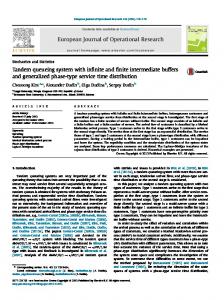
Example 1 We consider a system in which the service time, S , of each customer is a discrete random variable with sa = P { S = 8 ) as follows: s1 = 0.4; s2 = 0.2; sg = 0.1; sg = 0.3. 4. The vacation consists of two parts: the first part is a constant 5. time of 10 units and the second part is distributed according to a binomial distribution with parameters n = 12 and p = 0.25. The arrival process is Poisson with rate 0.1. 6. We study the behavior of this system for different values of the Target Cycle Time ( T C T ) , for the CL and the CLL Once we obtain the vector x, we can readily extract the policies. Fig. 1 through 3 present the mean waiting times and steady state distribution of the number of customers present the values of p = ?r,B for different TCT values. It can be observed from Fig. 1 and 2 that as the TCT is rein the system immediately after a customer is served and departs, as follows. Define the random variable ( as the indicator duced, both p and the mean waiting times go up. The increase function of the imbedding point which is a service completion, in p is fairly linear with decreasing TCT values. However, the mean waiting times display a marked increase as p nears unity. i.e., As discussed earlier, note that p is not equal to the offered load 1 if the imbedding point is a service completion, on the server, unless we let TCT approach infinity. Clearly, F = { 0 if the imbedding point is a vacation completion. as seen from the graphs, p is determined by the TCT. The graphs also indicate that for a given TCT value, the Define w,, n = 0 , 1 , . . . , as the steady state probability that values of p for the two policies are reasonably close to one there are n customers in the system immediately after a cusanother. However, as we continue to reduce TCT, there is tomer departs the system. Hence, a marked difference between the two mean waiting times, as the system begins to saturate. Fig. 3 presents the behavior of the mean waiting time for different values of p, under the two 3.
CHIARAWONGSE rr ul.: T H E M f G f l QUEUEING SYSTEM
1851
.
70
..
60-
6050
a
CL CLL
40. 30
20
22
24
26
28
30
-
32
34
-
0.6
0.7
TCT
0.8
P=lrs
Fig. 1; E[waiting time] as function of TCT for Example 1.
Fig. 3: Plot of p vs E[waiting time] for Example 1.
% I II
CL
0.8
20
1 .o
0.9
a
22
24
26
28
30
32
34
TCT
20
22
24
26
28
30
CLL
32
:
TCT
Fig. 2: p as a function of TCT for Example 1.
Fig. 4: E[queue length] at start of vacation in Example 1.
policies. Note that the different values of p are generated by the different TCTs. Fig. 4 presents the mean queue length at the instant the server begins a vacation, for different TCTs. Again, the mean queue lengths for the CL and the CLL policies are close to one another until the system begins to saturate, at which point the differences become markedly large. Fig. 5 presents the distribution of the queue length at the start of a vacation, for a TCT value of 22. Note, from Fig. 1 and 2, that the system is approaching saturation at this TCT value. Fig. 6 presents the distribution of the visit period of the server for a TCT value of 22. This distribution is of interest in modeling a system with multiple stations since it could be used to capture the distribution of the “vacation” the server takes from a given station in the multiple station system. As TCT increases, the size of the resulting model increases. For example, with TCT equal to 32, the dimension of each
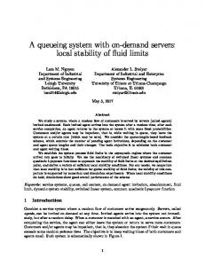
matrix A, and B v , v 2 0, was 357 by 357. With a stopping tolerance of 1E - 09, the resulting models required about 13 hours to execute. For large TCT values, however, it may be observed that the behavior of a model using either the CL or CLL policy would approach that of a standard exhaustive service vacation model. Hence, one may consider adopting the exhaustive service approximation for such cases. The FDDI Media Access Protocol As we have mentioned earlier, our CLL model can be used to analyze the FDDI protocol for performance measures such as the response time for asynchronous traffic with a single priority level at a station on the network when other stations generate only synchronous traffic. In order to validate the accuracy of our model in such a situation, we simulated a FDDI system with 13 stations and compared the results with those obtained from the M / G / l analytic model.
IEEE TRANSACTIONS ON COMMUNICAnONS, VOL. 42, NO. 21314, FEBRUARYMARCHIAPRIL 1994
1852
0.3
a0 II
CL
I
L,
4&
Simulation
O2
0.1
L
0.0 0 1 2 3 4 5 6
7 8 910111213141516171819202122 QueueLength
Fig. 5: Queue length distribution at start of vacation in Example 1.
0 1
2 3 4 5 6 7 8 9 10 11 12 13 14 15 16
Queue Length Fig. 7: Queue length distributions at Station 1 at the departure epochs of asynchronous packets for Example 2
15,000,000 time slots after a warm up period of 50,000 time slots. With an arrival rate of 0.1 packets/slot, approximately TCT = 22 1,500,000 packets thus passed through the system during the duration of the simulation. The above system was analyzed by modeling Station 1 as 0.2 a M / G / l queueing system with server vacations, which emF 9 ploys the CLL service discipline. The distribution of the vacas a n CL I tion period, which corresponds to the server’s switching time CLL and the service times of the synchronous packets at other stations, was approximatedby the vacation time distribution used 0.1 in Example 1. The mean sojourn times of asynchronous packets obtained from simulation and the matrix-analytic method were 17.560 and 16.139 slots, respectively. This gives a relative error of 0.0 approximately 8% compared to the simulation result. Compar0 1 2 3 4 5 6 7 8 9 101112131415 ison of the queue length distribution at the departure epochs Visit Period of the asynchronous packets are shown in Fig. 7. (Note that, by Burke’s Theorem, the queue length distribution seen by Fig. 6: Distribution of the visit period for Example 1. a departing customer is the same as that seen by an arrival customer which, by PASTA, is the same as the steady state distribution of the number of customers present in the system.) Example 2 In this example, we consider a FDDI system It can be observed that there is a close match between the two with 13 stations. Station 1 generates only asynchronous packdistributions. ets according to an independent Poisson process with rate 0.1 packetshlot. The service time at Station 1 is an independent and identically distributed discrete random variable, S , with Systems with Continuous Service Time and Vacathe same distribution as in Example 1, i.e. SI = 0 . 4 ; s ~ = tion Time Distributions 0 . 2 ; s 3 = 0 . 1 ; s 4 = 0 . 3 w h e r e s ~ = P { S = i } ,i = 1,2,3,4. We have developed a matrix analytic method which exactly The infinite buffer space for asynchronous packets is assumed analyzes the M/G/1 queueing systems with vacations where at Station 1. Stations 2-13 only generate synchronous pack- service time and vacation time distributions are discrete with ets. At each of these stations, a packet is generated every 16.9 finite supports. The model can also be used to analyze sysslots with probability 0.25, independent of packet generations tems with continuous distributions if these distributions can be at other stations. Each synchronous packet requires a service approximated by (bounded) discrete distributions fairly accutime equal to one slot. A single buffer space is reserved for rately. We experimented with several approaches and found synchronous packets at each station. Those packets which ar- that a discrete distribution which had the same first two morive and find the buffer occupied are lost. The cycle time limit, ments as the continuous distribution gave best results in terms TCT, is assumed to be 25 slots. The simulation was run for of closeness of fit. 0.3
CHIARAWONGSE rt al.: THE M/G/I QUEUEING SYSTEM
1853
We briefly describe how we obtain the probability mass function (pmf),P k , of a discrete random variable X, given the cumulative distribution function (cmf),F x , of a continuous random variable X , such that E [ X ] = E [ X ]and E [ X 2 ] = E [ X 2 ] . We first choose a value z such that P{X 5 z} 2 0.95. Let k = 1x1, and choose a slot size, A, such that we obtain a desirable number, n , of equally spaced points (slots) in the range (0, A]. We now determine a set of n unknowns, p i , i = 1 , 2 , . . . ~ nwhere , pi = P , which satisfy the following linear constraints.
Table 1: Discrete service time distributions with the same first two moments as their continuous counterpart for the data presented in Example 3
Distribution 1 Service Time I Probability 1 I 0.6467
I
n
c p ;
= 1.0,
i=l n
(b)
Distribution 2
i=l n
i=l
pi
2 0, v i .
(32)
Note that if n is large enough, there will always be more than one set of pi’s which satisfy the above set of linear constraints. Although, we do not have a conclusive way to select the best distribution from such a set, we observed, from several experiments, that all of them yield relatively similar results. Example 3 presents some of these results.
Service Time
Probability 0.2500 0.1875
Example 3 Consider an M / G / l queueing system with arrival
rate 0.1 customers/slot. The service time, S, is exponentially distributed with mean 2.3 slots. The vacation time, V, consists of two parts: the first part V,, is constant with duration 10 slots, the second part, V,, is exponentially distributed with mean 3 slots. The service discipline employed is CLL in which the cycle time limit, TCT, is 25 slots. Using the approach described above, we obtained several discrete distributions for Table 2 Discrete vacation time distributions with the same the service time, S, and the vacation time, V = V, Ve. first two moments as their continuous counterpart for the data We present three pmf’s for the discrete service time S, and presented in Example 3 two pmf‘s for the discrete vacation time V in Tables 1 and 2 respectively. Using different combinations of the discrete service time and Distribution 1 vacation time pmf’s given in Tables 1 and 2, we solved the reVacation Time I Probability sulting model numerically by the matrix-analytic method. We 0.5625 denote the model with the kth service time distribution from 0.2500 Table 1 and the Ith vacation time distribution from Table 2 0.1875 as System Al. The following four models were solved: System 11, System 21, System 31, and System 22. The results were compared with those obtained from the simulation of the system with continuous service and vacation time distribuI Distribution 2 tions. The simulation was run for 15,000,000 time slots after Vacation Time Probability a warm up period of 50,000 time slots. With an arrival rate of 0.1 customers/slot, approximately 1,500,000 customers passed 0.6806 through the system during the duration of the simulation. 0.0972 The following mean sojourn times of customers were obtained from the simulation and the analysis:
+
Simulation 20.691
System11 System21 System31 System22 21.701
21.796
22.354
21.672
~
1854
IEEE TRANSACTIONS ON COMMUNICATIONS, VOL. 42, NO. 21314, FEBRUARYMARCHIAPRIL 1994
1
0.3
0
0.2
3
53
BBB Simulation
E
0 system31 0.1
0.0 0 1 2 3 4 5 6 7 8 9 1011121314151617
0 1 2 3 4 5 6 7 8 91011121314151617
QueueLength
Queue Length
Fig. 8: Queue length distributions seen by a departing customer for Example 3. The matrix-analytic model uses service time distribution 1 from Table 1 and vacation time distribution 1 from Table 2
Fig. 9: Queue length distributions seen by a departing customer for Example 3. The matrix-analytic model uses service time distribution 3 from Table 1 and vacation time distribution 1 from Table 2
The relative error percentage of the numerical results range from 5% to 8% based on comparison with the simulation result. Two comparisons of the queue length distributions seen by a departing customer obtained from the analysis and from the simulation are shown in Fig. 8 and 9. Only two such comparisons are displayed since the queue length distributions from the other systems being analyzed were almost identical. It can be seen from the results that the system with the continuous service and vacation time distributions, presented in this example, is approximated and analyzed quite accurately, by our analytic model.
tivation behind such an extension is that in the FDDI protocol the TRT is known to be bounded. Hence, the time the token spends at a station and the time it is on the vacation immediately following this, are correlated. The proposed extension can be used to model this correlation more accurately.
V. CONCLUSIONS We have analyzed a M / G / l queueing system with vacations in which the sojourn time of the server at the queue is controlled by a timer. The service time of a customer and the vacation time of the server were allowed to only take on integer values. We identified an imbedded Markov chain at the completion instance of either a service or a vacation. Using the matrix-analytic approach, the model was solved to obtain the distributions for the number of customers present in the system at an arbitrary point in time, the time the server spends at the queue in each cycle, as well as the number of customers at the beginning of a vacation. Our model can also be used to approximately analyze the system with continuous service and vacation time distributions. By substituting the continuous service and vacation time distributions with discrete distributions obtained by matching the first two moments of these distributions, we can obtain fairly accurate approximation results. A straightforward extension to the queueing models we presented for the CL and CLL policies would be to allow the distribution of the server's vacation time to depend on the time the server spends at the queue just prior to the vacation. The mo-
tems, Ed. H. Takagi, Elsevier Science Publishers B.V. (NorthHolland), 1990. [3] F.E. Ross. FDDI - a tutorial. IEEE Communications Magazine, vol. 24, pp. 10-17, May 1986. [4] F.E. Ross. An overview of FDDI: The fiber distributed data interface. IEEE Journal on Selected Areas in Communications, vol. 7, pp. 1043-1051, Sept. 1989. [5] K.K. Leung and M. Eisenberg. A single-server queue with vacations and gated time-limited service. IEEE Transactions on Communications, vol. COM-38, pp. 1454-1462, Sept. 1990. [SI K.K. Leung and M. Eisenberg. A single-server queue with vacations and non-gated time-limited service. Performance Evaluation, vol. 12, pp. 115-125, Apr. 1991. [7] R.O. LaMaire. An M/G/f vacation model of an FDDI station. IEEE Journal on Selected Areas in Communications, vol. 9, pp. 257-264, Feb. 1991. [8] T.T. Lee. M / G / l / N queue with vacation time and limited service discipline. Performance Eualuation, vol. 9, pp. 181-190, June 1989. 191 K. Ghana. Performance modeling of token-passing networks with timLout mechanisms. Ph.D. Dissertation; Rensielaer Polytechnic Institute, Troy, NY, 1990. [lo] H. Takagi. Effects of the target token rotation time on the performance of a timed-token protocol. Performance '90 E&. P.J.B. King, I. Mitrani, and R.J. Pooley, Elsevier Science P u b lishers B.V. (North-Holland), pp. 363-370, Sept. 1990. [11] M.J. Johnson. Proof that timing requirements of the FDDI token ring protocol are satisfied. IEEE Transactions on Communications, vol. COM-35, pp. 620-625, June 1987.
REFERENCES [l] B. Doshi. Queueing systems with vacations: A survey. Queueing Systems, vol. 1,pp. 29-66, June 1986. [2] H. Takagi. Queueing analysis of polling models: an update. Stochastic Analysis of Computer and Commzlnication Sys-
-
1
CHIARAWONGSE et al.: THE M/G/l QUEUEING SYSTEM 1855
[12] K.C. Sevcik and M.J. Johnson. Cycle time properties of the FDDI token ring protocol. IEEE Transactions on Software Engineering, vol. SE-13, pp. 376-385, Mar. 1987. [13] D. Dykeman and W. Bux. Analysis and tuning of the FDDI medium access protocol. IEEE Journal on Selected Areas in Communications, vol. 6 , pp. 997-1010, July 1988. [141 W. Bux. Token-ring local-area networks and their performance. Proceedings of the IEEE, vol. 77, pp. 238-256, Feb. 1988. [15] M. T a n g e m a m and K. Sauer. Performance analysis of the timed token protocol of FDDI and FDDI-II. IEEE Journal on Selected Areas i n Communications, vol. 9, pp. 271-278, Feb. 1991, [16] K. Chang and D. Sandhu.Mean waiting time approximations in cyclic-server multiqueue systems with exhaustive limited service policy. PTOC.IEEE INFOCOM ’91, pp. 1168-1177, Apr. 1991. [17] S.W. F h a n n and Y.Wang. Analysis of cyclic service systems with limited service: bounds and approximations. PeTformance Evaluation, vol. 9,pp. 35-54, Nov. 1988. [18] M.F. Neuts. StTUCtUTed stochastic matrices of M / G / 1 type and their applications. Marcel Dekker, New York, 1989. [19] E. Cinlar. Introduction t o Stochastic PTOCCSSCS. Prentice-Hall, New Jersey, 1975. [ZO] V. Ramswami. A stable recursion for the steady state vector in Markov chains of M/G/1 type. Stochastic Models, vol. 4, no. 1, pp. 183-188, 1988. [21] R.B.Cooper. Introduction to Queueang Theory, 2nd ed. NorthHolland, New York, 1981. [22] R.W. WOW. Poisson arrivals see time averages. Operations Research, vol. 30, pp. 223-231, Mar.-Apr. 1982.
Jhitti Chiarawongse obtained his Ph.D. in Computer Science and Engineering from the University of Michigan in 1992. His current interests are analytical performance models for local and wide area computer networks. Mandyam M. Srinivasan is an Associate Professor in the Management Science Program at the University of Tennessee, Knoxville, TN. He received the Master of Technology degree from the Indian Institute of Technology, Madras, India, a Post-Graduate Diploma in Management (MBA) from the Indian Institute of Management, Bangalore, India, and a Ph.D. in Industrial Engineering and Management Sciences from Northwestern University. Dr. Srinivasan’s current research interests are in performance evaluation of computer networks and flexible manufacturing systems. He is a member of The Institute of Management Sciences and the Operations Research Society of America. He is an Associate Editor for the International Journal of Flexible Manufacturing System, and serves on the Editorial Review Board of Production and Operations Management.
Toby J. Teorey received the B S. (1964) and M.S. (1965) degrees in Electrical Engineering from the Universlty of Anzona, and the Ph D. (1972) in Computer Sciences from the University of Wlsconsm. He is currently Professor of EECS and Associate Chair for Computer Sclences and Engineering at the Unlverslty of Michlgan. He is author of two books on database deslgn, the most recent entitled Darabase Modeling and Design. Fundamental Principles , Morgan Kaufmann Pubhshers, 1994 (2nd Edition) Professor Teorey’s current research interests are object data modeling, dlstnbuted databases and dtrectortes, and network performance tools He directed the development of NetMod, a tool for network capacity planning and performance prediction that runs in the Macintosh HyperCard and PC Windows environments.