The metron model: elements of a unified deterministic theory of fields

arXiv:quant-ph/9606033v2 6 Aug 1996

The metron model: elements of a unified deterministic theory of fields and particles K. Hasselmann February 9, 2008

Contents 1

The Metron Concept 1.1 1.2 1.3 1.4

2

. . . .

. . . .

. . . .

. . . .

. . . .

. . . .

. . . .

. . . .

. . . .

Introduction . . . . . . . . . Identification of fields . . . Lagrangians . . . . . . . . . The Maxwell-Dirac-Einstein Particle interactions . . . .

. . . . . . . . . . . . . . . . . . . . . Lagrangian . . . . . . .

. . . . .

. . . . .

. . . . .

. . . . .

. . . . .

. . . . .

. . . . .

. . . . .

. . . . .

. . . . .

. . . . .

. . . . .

. . . . .

. . . . .

. . . . .

. . . . .

. . . . . .

. . . . . .

. . . . . .

. . . . . .

. . . . . .

. . . . . .

. . . . . .

. . . . . .

. . . . . .

. . . . . .

. . . . . .

. . . . . .

. . . . . .

. . . . . .

. . . . . .

. . . . . .

. . . . . .

Introduction . . . . . . . . Strong interactions . . . . Electroweak interactions . Invariance properties . . . Summary and conclusions

. . . . .

. . . . .

. . . . .

. . . . .

. . . . .

. . . . .

. . . . .

. . . . .

. . . . .

. . . . .

. . . . .

. . . . .

. . . . .

. . . . .

. . . . .

. . . . .

. . . . .

38 38 43 49 53

65

Introduction . . . . . . . . . . . . . . . Time-reversal symmetry . . . . . . . . The radiation condition . . . . . . . . The EPR paradox and Bell’s theorem Bragg scattering . . . . . . . . . . . . Atomic spectra . . . . . . . . . . . . .

The Standard Model 4.1 4.2 4.3 4.4 4.5

7 13 17 23

35

Quantum Phenomena 3.1 3.2 3.3 3.4 3.5 3.6

4

Introduction . . . . . . . . . . . . . . . . . . . . . . . Specific properties of the metron model . . . . . . . Development and implications of the metron concept The mode-trapping mechanism . . . . . . . . . . . .

The Maxwell-Dirac-Einstein System 2.1 2.2 2.3 2.4 2.5

3

3

68 68 73 84 88 94

109 . . . . .

. . . . .

. . . . .

. . . . .

1

. . . . .

. . . . .

. . . . .

113 114 126 137 141

The metron model: elements of a unified deterministic theory of fields and particles Part 1

The Metron Concept K. Hasselmann February 9, 2008

ABSTRACT In the first part of this four-part paper, the framework of a unified deterministic theory of fields and particles is presented. The model is based on a single set of field equations, Einstein’s vacuum equations for a higher-dimensional metric space. The extra space is not compactified, for example by assuming a spherical topology with very high extra-space curvature, the metric being represented as a perturbation superimposed on a flat-space background metric. It is proposed that the equations contain nonlinear soliton-type solutions, termed metrons, which are strongly localized in physical space, while carrying far fields which are independent of or periodic with respect to extra space and time. The solutions are generated through the mutual interaction between an inhomogeneous mean field (e.g. a gravitational or electromagnetic field), which acts as a wave guide, and a wave field, which is periodic in extra (harmonic) space and is trapped in the wave guide. The modetrapping mechanism is demonstrated for a simplified Lagrangian which reproduces the basic nonlinear properties of the gravitational Lagrangian while suppressing its tensor complexities. The more difficult task of computing metron solutions for the higher-dimensional gravitational system is not attempted in this paper. The model is strictly symmetrical with respect to time reversal. Thus Bell’s basic theorem on the non-existence of deterministic hidden-variable theories, which is based on the existence of an arrow of time, is not applicable. Time-reversal symmetry, Bell’s theorem and the metron interpretation of the EPR experiment are discussed in more detail in Part 3. Since the Einstein vacuum equations contain no physical constants, all particle properties (mass, charge, spin etc.) and physical constants (the gravitational constant, Planck’s constant, the electroweak and strong coupling coefficients, the parmeters of the Standard Model, etc.) are inferred from the properties of the metron solutions. The paradoxes of wave-particle duality are explained by the dual nature of the metron solutions. The localized, strongly nonlinear core regions of the solutions embody the corpuscular properties, while the metron far fields, including a periodic standing-wave de Broglie field, are responsible for the wave-like interference phenomena. The existence of discrete atomic spectra is explained by resonant interactions between the eigensolutions of the Maxwell-Dirac field equations and the orbiting electrons. Thus the metron picture of the atomic system represents an amalgam of QED (at the tree level) and Bohr’s original orbital theory. The principal properties of the Standard Model are reproduced assuming a four-or five-dimensional harmonic-space background metric. The Standard Model gauge symmetries are explained as a special case of the diffeomorphic gauge symmetries of the Einstein equations. Details are given in Parts 2 and 4.

Keywords: metron — unified theory — wave-particle duality — higher-dimensional gravity — solitons — Maxwell-Dirac-Einstein system — Standard Model — EPR paradox — Bell’s theorem — arrow of time

4

´ ´ RESUM E Dans la premi`ere partie de ce travail est ´elabor´e le cadre d’une th´eorie unifi´ee d´eterministe des champs et particules. Cette th´eorie s’appuie sur un ensemble unique d’´equations de champs: les ´equations d’Einstein du vide dans un espace `a dimensions au-del` a de quatre. Les dimensions additionnelles ne sont pas compactifi´ees par cons´equence d’une tr`es grande courbure de l’espace suppl´ementaire. La m´etrique est repr´esent´ee par une perturbation superpos´ee sur la m´etrique de fond de l’espace plat. Des solutions non-lin´eaires de type soliton appel´ee m´etrons, sont propos´ees pour ces ´equations. Elles apparaissent de fa¸con locale dans le domaine spatial et de fa¸con p´eriodique dans les dimensions suppl´ementaires ainsi que dans le domaine temporel. Les solutions r´esultent d’une interaction mutuelle entre un champ moyen inhomog`ene (par exemple un champ gravitationnel ou un champ ´electromagn´etique) agissant comme guide d’onde et un champ ondulatoire p´eriodique dans l’espace suppl´ementaire, dit espace harmonique captur´e dans le guide d’onde. Le m´ecanisme de capture de modes de champs est d´ecrit `a l’aide d’un Lagrangien simplifi´e, qui n´eammoins reproduit les propri´et´es fondamentales non-lin´eaires du Lagrangien de gravitation tout en supprimant la complexit´e des structures des tenseurs. Le but de ce travail se limite aux calculs des solutions au syst`eme de gravitation `a basse dimension, et non aux calculs plus compliqu´es des solutions du syst`eme complet de gravitation ` a haute dimension Le mod`ele est strictement sym´etrique au sein du domaine temporel. Ainsi le th´eor`eme fondamental de Bell, qui s’appuie sur l’existence d’une fl`eche du temps et qui ´etablit la non-existence d’une th´eorie d´eterministe `a variables cach´ees, n’est pas valable. La sym´etrie d’inversion temporelle, le th´eor`eme de Bell et l’interpretation de m´etron de l’exp´erience d’Einstein, Podolsky et Rosen (EPR) seront ´etudi´es en d´etail dans la troixi`eme partie. Puisque les ´equations d’Einstein du vide ne poss`edent pas de constantes de physique, on d´eduit toutes les propri´et´es de particules (masse, charge, spin, etc.) ainsi que les constantes de physique (constante de gravitation, constante de Planck, les coefficients de couplage des forces fortes et des forces faibles, les param`etres du mod`ele standard, etc.) ` a partir des propri´et´es des solutions de m´etron. Les paradoxes de la dualit´e onde - corpuscule s’expliquent par la nature duale des solutions de m´etron. Les r´egions localis´ees, fortement non-lin´eaires du noyeau des solutions, poss`edent les propri´et´es corpusculaires, tandis que les champs de m´etron `a distance, y compris un champ p´eriodique d’onde stationnaire de de Broglie , sont responsables de l’aspect ondulatoire des ph´enom`enes d’interf´erence. L’existence de spectres atomiques discrets s’explique par les interactions r´esonantes des les solutions propres des ´equations de champs de Maxwell-Dirac et des ´electrons tournoyants. Ainsi l’aspect de m´etron d’un syst`eme atomique repr´esente-t-il un amalgame entre la QED (si l’on exclut de la s´erie de perturbation les diagrammes de Feynman qui contiennent des boucles) et la th´eorie quantique originelle des orbites de Bohr. Les propri´et´es principales du mod`ele standard sont reproduites, ´etant donn´ee une m´etrique de fond de l’espace harmonique ` a quatre ou cinq dimensions. Les sym´etries de jauge du mod`ele

5

standard sont ici des cas particuliers des sym´etries de jauge diff´eomorphiques des ´equations d’Einstein (cf. parties 2-3-4).

Mots cl´ es: m´etron — th´eorie unifi´ee — dualit´e onde-corpuscule — th´eorie de gravitation `a haute dimension — solitons — syst`eme de Maxwell-Dirac-Einstein — mod`ele standard — paradoxe d’EPR — th´eor`eme de Bell — fl`eche du temps

6

1.1

Introduction

Quantum indeterminacy versus classical objectivity Despite the impressive achievements of quantum theory, the discusssion on the conceptual foundations of the theory has never completely abated ever since the theory was first conceived nearly seventy years ago [1]. The debate has revolved around a number of unusual and somewhat disturbing features of the theory: the limitation to a purely statistical description of microphysical systems already at the fundamental level of the basic equations; the associated inability of describing individual microphysical ‘events’ or assigning physical ‘objects’ to the mathematical quantities appearing in the basic equations; the imprecise demarkation between the quantum physical system and the macrophysical system described by classical physical observables; and the concept of a measurement process which induces a sudden collapse in the quantum physical state vector. These difficulties, together with the problem of divergences, have not only been a continual source of concern in the development of quantum field theory, but have also presented an obstacle to the unification of quantum field theory with the general relativistic theory of gravitation, which, in its elegantly simple foundation on the postulate of invariance with respect to coordinate transformations, is free of these conceptual intricacies. Ultimately, the quantum theoretical controversy between deterministic ‘realism’ and probabilistic ‘positivism’ reduces to the pivotal question: have we no choice but to resort to a fundamentally statistical description of nature at the microphysical level, or is it conceivable that a deterministic theory can be constructed which provides an objective description of individual microphysical events? The alternative viewpoints can be illustrated by the example of the Bragg scattering of a monochromatic beam of particles at a periodic lattice. Quantum theory predicts the mean intensities of the scattered beams in the various discrete Bragg scattering directions, but is unable to ‘describe’ what actually happens when an individual particle is scattered. Yet for a sufficiently low-intensity particle beam, it is perfectly possible to uniquely reconstruct (to adequate accuracy within the Heisenberg uncertainty constraints) the path of an individual particle, which can be registered when it leaves the particle source, must pass through the (small) lattice target and is detected again at a later time, after it has been scattered into some particular Bragg direction, by some (also small) element of a counter array. Quantum theory nevertheless continues to describe such an individual event by a scattering wave function which contains all the possible Bragg beams up to the instant when the location of the scattered particle is actually measured, at which instant the wave function is suddenly collapsed to a new state function describing the localized particle state. The Copenhagen interpretation of a sudden collapse can be replaced by the more modern representation of a continuous evolution of the state function during the measurement process, but this does not change the quantum theoretical picture of a single particle scattering into a number of separate beams prior to the measurement process. In contrast, a deterministic particle theory should be able to mathematically describe (although not necessarily predict) such an individual scattering event in terms of the same

7

‘objective’ particle picture which an experimental physicist would normally use to describe the event. We come back to this example later. The basic paradigm of quantum theory is that the experimental finding of both wave-like and corpuscular phenomena at the microphysical level is fundamentally irreconcilable within the framework of classical ‘objective’ physics. The quantum theoretical solution is to ignore all corpuscular properties at the basic level of the dynamical system equations, which describe only nonlinearly interacting wave fields. To establish the connection to the dual nature of observed microphysical phenomena, a suitable statistical interpretation of the wave-field computations is then introduced. This enables the wave-dynamical computations to be related to either waves or particles, depending on the experimental situation. However, the ‘objective’ simultaneous ‘existence’ of both waves and particles is denied. In the following we question this paradigm. It is argued that the dual existence of both wave-like and corpuscular properties does not necessarily contradict ‘objective’ physics in the classical sense. We develop the basic elements of a theory of fields and particles which explicitly incorporates both waves and particles as objective phenomena in a conceptually simple manner. The widely held view that such theories are inherently incompatible with the experimental evidence, as exemplified by Bell’s theorem, is shown to be invalid for the present model.

The metron approach The model contains two basic elements: (i) it is shown that the apparent waveparticle duality conflict can be resolved in terms of a rather simple soliton-wave picture which exhibits both wave-like features, represented by a periodic far field of the soliton, and particle features, associated with the strongly nonlinear core region of the soliton; and (ii) a specific soliton model is developed which unifies gravity with the other forces of nature. The model is based on a single simple fundamental equation, Einstein’s gravitational field equation in a higher-(eight- or nine- )dimensional matter-free space, without a cosmological term: RLM = 0 (1.1) where RLM is the Ricci curvature tensor. Apart from the trivial flat-space solution, Einstein’s vacuum equations have solutions, such as gravitational waves, for which the Ricci contraction of the Riemann curvature tensor but not the full curvature tensor itself vanishes. We postulate that the higher-dimensional equations possess also nonlinear soliton-type wave solutions, referred to in the following as metrons. The determination of the metron solutions themselves is a major computational task and is not attempted in this four-part paper. However, after summarizing the principle concepts and properties of the metron model in the first three sections of Part 1, we present in Section 1.4 some explicit computations of solitons of the same nonlinear structure as the proposed metron solution for a simpler nonlinear system which exhibits the same features as the gravitational equations without their tensor complexities. The main purpose of this exploratory paper, developed in Parts 2-4, is to demonstrate that the equations (1.1) have an extremely rich nonlinear structure which encompasses all the principal interactions of quantum field theory and can be 8

used as the foundation of a unified deterministic theory of fields and particles. This is shown for electromagnetic interactions, i.e. for the Maxwell-Dirac-Einstein system, in Part 2 and for all forces, including weak and strong interactions, in the discussion of the Standard Model in Part 4. Based on the analysis of the Maxwell-DiracEinstein System, Part 3 addresses basic issues of microphysics and quantum theory, such as irreversibility, the EPR parodox, Bell’s theorem, wave-particle duality and the origin of discrete atomic spectra. We note that matter is not included as a separate external source term in (1.1). Mass and other particle properties are derived instead as properties of the solutions of the field equations themselves [2]. The physical spacetime components of the Ricci tensor contain not only the Ricci tensor for the four-dimensional gravitational field but in addition (strongly nonlinear, localized) terms arising from the contraction of the extra-space components of the Riemann tensor. It will be shown that these yield the standard energy-momentum tensor which appears as external source term in classical four-dimensional gravitational theory. Electromagnetic forces and weak and strong interactions are represented by the further extra-space or mixed physical spacetime-extra-space components of the Ricci tensor. These can similarly be decomposed into linear or weakly nonlinear far-field contributions and strongly nonlinear localized terms, the latter representing in this case the currents arising from electric charges and weak and strong interactions. Thus all forces follow, as in classical general relativity, from the curvature of space. However, the curvature is not produced by prescribed mass fields, but is a self-generated feature of the nonlinear field equations (1.1) themselves. Moreover, in contrast to the standard field theoretical approach, the coupling constants and symmetries are not postulated in the basic field equations, but follow from the specific geometrical properties of the metron solutions. The basic equations are free of physical constants, and the only postulated symmetry is the invariance of the field equations with respect to coordinate transformations. The choice of (1.1) as the fundamental set of equations follows naturally from three considerations: 1. In order to develop a unified description of all forces we wish to adopt Einstein’s successful and elegant approach of identifying forces with curvature in space. Since the metric of four-dimensional spacetime is already fully needed to describe classical gravity, the inclusion of additional forces represented by metric fields requires an extension of space to higher dimension. 2. We wish ultimately to explain the particle spectrum, including the particle masses. This can clearly not be achieved by a theory in which mass is postulated to exist from the outset. The mass-dependent source term in the Einstein equation must therefore be omitted, the properties of mass (and other particle properties) being derived from the solutions of the nonlinear Einstein vacuum equations themselves. 3. The equations should be consistent with the principle of maximal simplicity.

9

The present approach clearly lies outside the main stream of modern unification schemes. Rather than trying to unify gravity and quantum theory by quantizing gravity [3], we attempt to apply the concepts of (higher-dimensional) gravity theory to explain quantum effects. Thus our starting point is the Kaluza-Klein approach of the twenties rather than the super-gravity and super-symmetry theories of the eighties. The theory contains a number of common elements with previous attempts to develop a classical description of microphysical phenomena. As in Bohm [4] and de Broglie [5], wave-like and particle-like properties are not regarded as contradictory and mutually exclusive phenomena, but as simultaneously existing ‘objective’ realities in a classical, deterministic sense. However, in contrast to the de Broglie-Bohm pilot wave theory, waves and particles are not treated as separate entities, but appear rather as the near and far field expressions of the same physical object: a finite particle, or ‘metron’. The description of particles as objects of finite extent is clearly reminiscent of the early attempts of Lorentz [6] to develop a theory of the electron as a finite-sized charge distribution. The present particle model differs from that of Lorentz in containing more space dimensions and more fields. The particles consist of a localized, strongly nonlinear core and a set of linear far fields which, in the particle rest frame, are either time independent (gravitational, electromagnetic and neutrino fields) or periodic in time (de Broglie waves). A transitional weak interaction region bridges the strongly nonlinear core and linear far field regions. The core is the origin of the corpuscular properties of matter, while the periodic de Broglie far fields give rise to the wave-like interference phenomena. The de Broglie far field represents a trapped standing-wave field, so that radiative damping does not occur. These properties apply to physical spacetime. With respect to the extra-space dimensions, the metron fields are multi-periodic: they consist of a superposition of a finite number of fundamental periodic components and their higher-harmonic interaction combinations (including zero-wavenumber fields). Different Fourier components are identified with the different constituents (partons) of elementary particles, which will be related in Part 4 to the partons of the Standard Model. All interaction fields are regarded as perturbations superimposed on an ndimensional background metric ηLM = diag (1, 1, 1, −1, · · · , ±1, · · ·). In contrast to most modern Kaluza-Klein theories, the extra space is not compactified by assuming a spherical topololgy with a background metric of very large curvature. The concept of periodic fields with respect to extra-space dimensions goes back to the original Kaluza-Klein papers [7] and is revived in recent string theories [8]. To emphasize the role of periodicities in extra-space and the fact that the present extra-space is more closely related to the periodic extra-space dimensions of string theory than the usual curvature-compactified extra-space of higher-dimensional gravity, we shall refer to extra space in the following as harmonic space. The assumption that all fields can be treated as perturbations with respect to a flat background metric implies that the description is local with respect to cosmological scales. The manner in which this local description is embedded in a cosmological model of n-dimensional space is not discussed. Similarly, the origin of the distinction in the structure of the perturbation fields with respect to physical 10

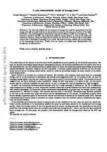
Ph ica ys lS pa ce

nic rmo

ce

Spa

Ha

ica

ys

Ph e

ce

pa

lS

pac

S onic

m

Har

Figure 1.1: Schematic diagram of trapped-mode (upper panel) and wave-guide (lower panel) components constituting a metron particle spacetime and harmonic space - a fundamental question of Kaluza-Klein theories which is usually deferred to cosmology - is not considered. It is simply noted that in a higher-dimensional space with the assumed background metric ηLM , trapped-mode particle-like solutions of (1.1) which are locally concentrated in the three dimensions of physical space and periodic with respect to the remaining dimensions can be expected to exist. The geometrical distinction between the locally concentrated and periodic properties of the metron solution defines the local physical spacetime and harmonic-space orientation. The vielbein can in general be a function of spacetime: different particles at different locations can have different vielbeins with respect to a non-local coordinate system. The changes in vielbein orientation are the origin of forces between particles (see also item 4 below) [9]. These general metron properties are inferred from the nonlinearity of the field equations (1.1). It is postulated (and demonstrated for a simpler prototype system) that the equations can support nonlinear soliton-type solutions in the form of wave modes trapped within a wave guide. The wave modes themselves generate the wave guide in which they propagate (cf. Fig. 1.1). The basic mechanism is a mutual interaction between the wave modes and the mean metric field which governs the wave propagation properties. The wave-guide and trapped modes are uniform in harmonic space and time but inhomogeneous with respect to physical space, the fields increasing to large values within the particle core and falling off exponentially 11

(in accordance with a trapped mode) or as 1/r (corresponding to a free wave) away from the core region. The mean ‘radiation stresses’ or currents arising from quadratic and higher-order wave-wave interactions are therefore inhomogeneous in physical space and distort the mean metric field in which the modes propagate. This produces a wave guide which refracts and traps the waves in the neighbourhood of the particle core. The increase of the trapped-mode amplitudes towards the particle core is in turn the origin of the inhomogeneous radiation stresses required to maintain the wave-guide. The mechanism is demonstrated for a prototype nonlinear Lagrangian obtained by projection of the full gravitational Lagrangian onto a finite set of modes. The reduced Lagrangian captures the basic nonlinear properties of the complete gravitational Lagrangian while ignoring its tensor complexities. As pointed out, the computation of metron solutions for the full gravitational equations is considerably more difficult and will not be attempted here.

Bell’s theorem and time-reversal symmetry A deterministic particle model with these properties clearly falls in the class of hidden-variable models and must therefore contend with the widely held view that hidden-variable theories are generically incompatible with quantum theory and experiment. Although von Neumann’s [10] celebrated proof that all hidden-variable theories are necessarily inconsistent with quantum theory has been shown by Bell [11] to rest on invalid assumptions, Bell’s [12] own well-known theorem on the EinsteinPodolsky-Rosen paradox [13] is generally cited as an irrefutable argument against hidden-variable theories. Bell showed that any hidden-variable interpretation of the EPR-Bohm experiment, in which a two-particle state with zero net angular momentum decays into two separate particles of opposite spin orientation, must satisfy an inequality relation regarding the correlations of the spins of the final particle states, measured in two arbitrary directions, which is in conflict with the quantum theoretical result and experiment. However, an essential assumption of Bell’s theorem, already emphasized by Bell, is forward causality, or the existence of an arrow of time. Although seemingly self-evident in the context of the EPR experiment, forward causality is in fact incompatible with time symmetry, which is a fundamental property of all basic (deterministic) equations of classical physics. Time-reversal symmetry is also a basic feature of the metron model. Bell’s theorem is therefore not applicable to the metron model, and it will be shown that the EPR paradox can indeed be readily resolved in the metron picture without violating the experimental findings. We shall adopt the classical view that an arrow of time does not appear at the basic level of microphysical phenomena but only at the aggregrated level of macrophysics: irreversibility arises through the introduction of time asymmetrical statistical hypotheses, such as the Boltzmann-Gibbs assumption that fine-grained structure properties can be neglected when going forwards in time, but not when reconstructing the past. While this view is generally accepted for classical wave-wave interactions or non-relativistic local particle interactions (collisions), the question of the time-symmetry of non-local interactions between particles mediated by fields 12

which propagate - as required for Lorentz invariance - at finite speed has been the subject of some debate. The problem is to explain the observed irreversible radiative damping of charged particles under non-uniform acceleration. Ritz [14] believed that this could be recovered only by introducing the auxilliary axiom that the electromagnetic field of a charged point particle is given by the retarded potential. Einstein [15], Tetrode [16] and others argued, however, that one should retain time symmetry by choosing the time-symmetrical Green function, consisting of half the sum of the retarded and advanced potentials. Einstein explained the observed radiative damping by the time-asymmetrical statistical properties of other particles with which the radiating particle interacts [17]. According to this view, an electromagnetically isolated charged particle would not emit radiation. The time-symmetrical theory of elecromagnetically interacting point particles has been developed further by Tetrode [16], Frenkel [18], Fokker [19], Dirac [20], Wheeler and Feynman [21], [22] and others, leading to the prevalent view that the classical electromagnetic coupling of particles interacting at a distance should in fact be described by time-symmetrical potentials. Radiation damping is explained by the time-asymmetrical statistical properties of a distant perfect absorber [21]. Alternatively, one can invoke the time asymmetry of the large-scale cosmological properties of an absorbing universe [23]. We shall similarly describe deterministic interactions between particles by timesymmetrical potentials, interpreting irreversibility as a statistical phenomenon (the cosmological interpretation is not at our disposal, since we have limited ourselves to a locally flat sub-region of the universe – although it could be argued that local statistical time-asymmetry can be justified ultimately only by cosmology [24]. However, in contrast to classical theories for point particles, we are not forced to take an axiomatic stance on this question. The only basic equations of the present theory are the (time symmetrical) set of equations (1.1). As solutions of these equations we can in principle admit particle states which have either time-symmetrical or time-asymmetrical far fields. It will be shown that the time-symmetrical particle solutions are closed in the sense that they conserve 4-momentum within a finite set of interacting particles, while the time-asymmetrical solutions are open, losing (or gaining) 4-momentum through radiation to (or from) space. It will be shown further, following the arguments of Wheeler and Feynman [21], that the open solutions of a finite set of interacting particles correspond to the closed solutions of an extended system including a distant ensemble of perfectly absorbing particles. Thus our option of describing particle coupling always in terms of time-symmetrical closed interactions, introducing an additional perfect absorber if required, is a matter of conceptual convenience rather than necessity. Depending on the system, interactions between particles can be described either in closed or open form. It will be argued that for the EPR experiment the closed rather than the open interaction description is appropriate.

1.2

Specific properties of the metron model

Starting from the basic assumption of the existence of trapped modes of the ndimensional gravitational equations, we develop in the following the framework of a

13

unified, deterministic, time-symmetric theory of fields and particles which is characterized by the following properties [25]. 1. All fields and particles are derived from the matter-free full-space gravitational equations (1.1) without introduction of additional fermion, boson or other mixed fields (in contrast to most modern higher-dimensional gravity theories [26]). Bosons and fermions are identified with particular components of the full-space gravitational metric. The theory is thus a pure higher-dimensional extension of Kaluza-Klein theory [7]. 2. The theory is developed by expansion of (1.1) about a flat space background metric ηLM = diag (1, 1, 1, −1, · · · , ±1, · · ·). Thus the harmonic space is not compactified. For much of the analysis concerned with the Maxwell-DiracEinstein system, the space dimension n (> 4) and the structure of ηLM in harmonic space need not be specified. However, in order to represent fermion fields in accordance with the standard Dirac Lagrangian, the dimension of harmonic space must be at least four. The Maxwell-Dirac-Einstein Lagrangian can then be recovered for a background harmonic-space metric of suitable signature. The principal features of electroweak and strong interactions, as summarized by the Standard Model, can also be obtained with a minimal four-dimensional harmonic-space representation, but a closer correspondence can be established if an additional dimension is introduced (see item 13 below). 3. The theory contains no universal physical constants or particle parameters. The only information on the structure of the physical world introduced at the axiomatic level is in the form of the gravitational equations (which in the matter-free form (1.1) contain no physical constants), in the dimension of space, and in the signs of the normalized background metric. The normalization of the background metric defines the length scales of physical space, time and the relative length scales of harmonic space. Once the reference length scale has been specified, for example in terms of the length scale of some reference particle, all other particle length and time scales, masses, spins and magnetic moments, Planck’s constant, the elementary charge, the gravitational constant and other coupling constants are determined by the intrinsic geometrical properties of the metron solutions [27]. The metron theory must therefore be able to explain, among other properties, the force hierarchy, including, in particular, the extremely small relative magnitude of gravitational forces. Although detailed metron solutions will not be presented in this paper, it will be shown that gravitational coupling is indeed an exceptionally weak higher-order nonlinear property of the metron solutions. 4. The only fundamental symmetry of the theory is the invariance with respect to regular coordinate transformations (diffeomorphisms). All other symmetries, such as the gauge symmetries of the Standard Model, follow from this very general gauge symmetry and the internal geometrical symmetries of the metron solutions. Thus, in contrast to the standard quantum-theoretical approach, specific symmetries are not introduced into the basic field equations, 14

but are derived from the specific geometrical properties of the solutions of the field equations. The geometry of the metron solution for a given particle defines a canonical local coordinate system in harmonic space at the location of the particle. This is the coordinate system for which the harmonic wavenumber vectors associated with the various periodicities of the metron solution are oriented in specific harmonic-space directions assigned to the individual forces. The gauge symmetries express the property that these local vielbeins can in general be functions of physical spacetime. As in the special case of classical gravitation, the connections describing the variations of the vielbeins in physical spacetime determine the forces between particles. 5. Consistent with the general philosophy of attributing specific symmetries to the solutions of the field equations rather than the field equations themselves, parity violation is explained as a spatial-reflection asymmetry of certain subcomponents of the metron solution, not as a reflection asymmetry of the weakinteraction sector of the basic Lagrangian. The phenomenon of parity violation is thus removed from the fundamental level of the field equations and – just as circularly polarized light or left-handed molecules – is not in conflict with our intuitive expectation that physics should be invariant with respect to spatial reflections [28]. Although not discussed, the phenomenon of CP violation in kaon decay can be similarly interpreted as a symmetry-breaking property of the metron solutions rather than of the basic Lagrangian. 6. All metron particles have finite mass. This is shown to be proportional to the metron rest-frame frequency in accordance with de Broglie’s relation. Finitemass particles support periodic (de Broglie) far fields. These are the origin of the wave-like interference properties of microphysical phenomena. The classical view that periodic far fields necessarily lead to irreversible radiative damping is invalid on the microphysical scale, where time symmetry prevails, the de Broglie far fields representing undamped trapped standing waves. 7. All far fields originate in individual metrons, or are generated by nonlinear interactions between fields in the vicinity of metrons. Free radiation fields without an associated metron source do not occur. The fields of individual particles are time-symmetrical (no net ingoing or outgoing radiation). Outgoing radiation fields, as mentioned above, are explained by interactions with a non-time- symmetrical statistical ensemble of absorbing particles. 8. Zero-mass particles (photons, neutrinos - assuming their rest mass is indeed zero) are not regarded as particles in the metron picture but as far fields in the classical sense. They derive their particle-like properties from the discrete transitions between discrete particle states which they mediate [29]. 9. The distinction between Einstein-Bose and Fermi-Dirac statistics for elementary particles – which plays a fundamental role in quantum field theory, where it is founded on the different commutation/anti-commutation relations for bosons and fermions – follows in the metron model simply from the distinction between finite-mass fermion particles, which as real particles cannot be 15

superimposed locally and therefore automatically comply with Pauli’s exclusion principle, and massless boson fields, which, as classical fields, can be superimposed without restriction. Exceptions from these categories, however, are the neutrino, which is a fermion but, according to the metron model, a field, and should therefore not underly the exclusion principle, and the finitemass electroweak bosons, which cannot be superimposed. The implications of these exceptions need to be explored further. 10. The theory, if meaningful, should encounter no divergence problems: the full set of all nonlinear interactions should yield finite, singularity-free particle states. The historical basis for this anticipation is not encouraging. Most nonlinear-interaction Lagrangians which have been considered in elementary particle physics have led to divergence problems, many of which could not be ‘repaired’ by renormalization methods. The nonlinear gravitational equations in four-dimensional spacetime (with mass source terms) are also prone to generate fields which are not globally regular (e.g. the Schwarzschild solution) - although it is encouraging that Christodoulou and Klainerman [30] have recently shown that Minkowski space is at least stable to small perturbations. 11. In contrast to quantum field theory, which is essentially a theory of fields, the metron model has both a field content, represented by the particle far fields, and a genuine particle content, represented by the strongly nonlinear core regions of the fields. This is the principal difference between quantum field theory and the metron model. Quantum field theory ‘resolves’ the paradox of wave-particle duality by in effect ignoring corpuscular properties in the basic dynamical field equations, which are pure wave equations. The connection to particles is established subsequently through an appropriate statistical formalism. Since particles do not appear explicitly in the theory, the concept of a ‘particle’ is not defined. In the metron model, on the other hand, both particles and fields are well defined ‘objects’ which can be identified with particular features of the solutions of the basic field equations. The particle content of the metron model yields the particle constants, coupling coefficients and (dimensionless) physical constants. The field content is formally equivalent (to lowest interaction order at the tree level) to the quantum field equations and therefore reproduces most of the basic results of quantum field theory. None the less, interactions between the corpuscular features (contained in the core regions) and field properties (represented by the far-field regions) of the metron model can be expected to yield different results from standard quantum field theory at higher order, for example in the computation of scattering and interaction cross-sections and branching ratios. These could provide a critical test of the theory (in addition, of course, to the derivation of the particle properties and dimensionless physical constants from the metron solutions). 12. In the metron picture it is meaningful to consider conceptually the simultaneous position and momentum of an objectively existing metron particle. Nevertheless, Heisenberg’s uncertainty principle is satisfied in the sense that metron particles are of finite extent and support de Broglie fields whose wavenum16

ber widths and spatial extent are in accordance with the Heisenberg relation. Moreover, it is in general not possible to devise an experiment in which an initial statistical distribution of metron particles with a joint momentum-position probabilty distribution satisfying the Heisenberg inequality relation is modified in such a way that the Heisenberg inequality relation is subsequently violated. Thus although the Heisenberg uncertainty principle applies formally only to the field content of the metron model, the traditional explanation of the uncertainty principle in classical particle terminology applies also to the metron model: it is not possible to accurately measure conjugate particle properties because of the interaction of the measurement device with the object being measured. 13. The principal features of the Standard Model can be reproduced assuming a suitable geometrical structure of the metron solutions and a four-dimensional harmonic space with background metric of suitable signature. A closer correspondence can be achieved, however, if an additional dimension is introduced. Nevertheless, despite the close structural similarity of the metron model with the Standard Model, small differences exist. In particular, the Standard Model interactions represent only a sub-set of all possible interactions in the gravitational system. Thus from the metron viewpoint the Standard Model appears only as a first approximation of the fully nonlinear system. A theory with these properties must clearly rest ultimately on the demonstration that the n-dimensional gravitational field equations do indeed support stable, selftrapping wave-guide type soliton solutions. The metron solutions must furthermore reproduce all known elementary particles and their interaction cross-sections and yield all physical constants. It is also clear that the development of such a complete theory, involving the numerical solution of the highly complex nonlinear n-dimensional gravitational equations, is not a minor undertaking. Before embarking seriously on this task, it therefore appears appropriate to consider first a number of general implications of the proposed alternative view of microphysical phenomena. This is the principal purpose of this first four-part paper. In short, we focus here on the feasibility of developing a model with the properties listed above rather than on the detailed structure of the model itself. Perhaps it would therefore be more appropriate to speak of the metron program rather than the metron model. Nevertheless, in the process of analyzing the basic concepts of the metron model, it will be found that most of the basic properties listed above can indeed be explicitly derived, although some of the stated features of the model must necessarily remain speculative at this stage.

1.3

Development and implications of the metron concept

The principal differences between the metron and quantum field theoretical view of microphysics are summarized in Table 1.1. The four parts of the paper are structured 17

in accordance with the phenomena listed in the table, the last column of the table indicating the sections in which the various concepts are discussed. Before commencing with a more detailed analysis of the metron concept in Parts 2-4, we first investigate in the remaining sections of Part 1 whether the basic premise of the theory, namely that the nonlinear gravitational field equations in a higherdimensional space can support self-trapping wave-guide modes, appears reasonable. It is demonstrated that trapped-mode solutions do indeed exist for nonlinear Lagrangians in n-dimensional space. Solutions are computed to lowest interaction order for a prototype nonlinear Lagrangian whose general structure follows from the gravitational Lagrangian by projection of the fields onto a reduced set of modes. Depending on the form of the coupling, the wave-guide can support trapped wave modes which fall off exponentially within a short distance outside the core (representing a model for quark and gluon fields or weak-interaction bosons) or far fields which decrease aymptotically as 1/r (gravitational and electromagnetic fields) or at a very weak exponential rate (de Broglie fields). Not resolved is the problem of the discreteness of the particle spectrum. The trapped-mode solutions found for the simplified Lagrangian generally represent a continuum. Additional considerations, such as stability, need to be invoked to reduce the solutions to a discrete set. We regard this as the major open problem of the metron approach at this point. Included in the question of discreteness is the problem of uniqueness. It must be shown that different particle states at different locations are not only discrete but also identical. A trivial continuum of solutions always exists because of the invariance of eq. (1.1) with respect to an arbitrary common change of the coordinate scales (without changing the fields – this follows from the homogeneity of the field equations with respect to the derivatives and is independent of the invariance with respect to diffeomorphisms). It must therefore be shown that all solutions exhibit the same spatial scaling (which can then be used to define a universal unit of length). This requires some form of multi-particle interaction leading, presumably, to some collective stability criterion. An alternative philosophy is to simply postulate (in analogy with string theory) that all solutions of the n-dimensional gravity equations in our world are periodic, with different but universal periodicities represented by different harmonic wavenumber vectors. The wavenumber components define the coupling coefficients of the electroweak and strong forces. The coupling coefficients can then no longer be regarded as derived quantities of the metron model, but appear rather as empirical universal constants (gravitational forces, however, will still be derived as higher order nonlinear metron properties). Which of the two views is more appropriate must await more detailed stability investigations (cf.[9]). In Part 2 the metron picture of the Maxwell-Dirac-Einstein system is developed. Assuming that trapped-mode solutions of the n-dimensioal gravitational equations exist, and that they are indeed discrete and unique, we address first the question whether it is possible to derive the basic boson spin-one and fermion half-odd-integerspin fields of standard quantum field theory from the tensor fields of the gravitational metric. In most higher-dimensional gravity theories, boson and fermion fields (as well as a large number of auxiliary mixed fields) are simply introduced as additional fields. In Sections 2.1, 2.3 it is shown that for a metron solution composed of fields 18

Phenomenon particles fields

Lagrangians

physical constants Bell’s theorem wave-particle duality atomic spectra absorption and emission divergences

Standard Model

gauge symmetries

particle interactions

QFT

Metron model trapped mode solutions defined statistically of field equations defined statistically in form nonlinear particle conjunction with parti- core, experienced as farfields cles by system state inferred from n-dimenderived from postulated sional gravitational Lagauge symmetries grangian derived from metron solutions with postulated postulated periodicities violates time symmetry of both theories, not applicable to reversible microphysical phenomena statistical interpretation; explained by periodic de non-existence of ‘objec- Broglie far fields of ‘objective’ particles tive’ fields and particles same as QED at loweigensolutions of est order augmented by Maxwell-Dirac system Bohr-orbiting electrons secular (resonant) persimilar formalism for turbations of system classical fields state renormalization ? (should not arise) general structure reprosummarizes parti- duced for given symcle spectrum, 19 empiri- metries of metron solutions; parameters detercal parameters mined by solutions inferred from geometrical symmetries of metron solutions and invariance postulated with respect to coordinate transformations not discussed, similarity to S-matrix formalism anticipated from analogy S-matrix formalism with optical absorption and emission

Sections 1.4, 2.5 2.4, 4

2.4, 4

2.5, 4 3.4 3.5, 3.6

3.6

3.6 –

4

2.4, 4.4

3.6

Table 1.1: Relation between metron and quantum field theoretical picture of microphysical phenomena 19

which are periodic in harmonic space, the familiar free-field equations for bosons and fermions can be extracted directly from the gravitational field equations. Assuming a suitable background harmonic-space metric with dimension of at least four and a periodicity of the fermion fields characterized by a single harmonic wavenumber vector k = (k5 , 0, 0, · · ·), say, the standard fermion-electromagnetic interaction Lagrangian for these fields is then derived using simple covariance arguments; an analogous form follows for the fermion-gravitational interaction Lagrangian. The U (1) gauge invariance of the Maxwell-Dirac-Einstein system is derived from the invariance of the metron solutions with respect to arbitrary spacetime-dependent translations in the x5 -direction. Progressing from the standard interaction Lagrangians for weak field-field interactions derived in Sections 2.3, 2.4, Section 2.5 considers the coupling between particles. This is described by the interactions of the fields in the nonlinear particle-core regions with the far fields of other particles. The classical Tetrode-Wheeler-Feynman description of point-particle interactions at a distance for electromagnetic and, by extension, gravitational interactions is recovered. In the process, the analysis yields expressions for the particle mass and charge, the gravitational constant, Planck’s constant and de Broglie’s relation. Similarly, all particle properties and physical constants are derived as functions of the metron solution. The exceedingly small ratio of gravitational to electromagnetic forces is explained by the metron geometry: coupling through the gravitational mass is found to be a higher-order nonlinear process than the coupling through the electromagnetic charge. The analysis of electromagnetic interactions in Part 2 can be generalized to weak and strong interactions by considering fermion fields with periodicities characterized by wavenumber vectors oriented in other directions than the electromagnetic direction k = (k5 , 0, 0, · · ·). However, before extending the analysis to the metron interpretation of the Standard Model in Part 4, we address first in Part 3 some of the conceptual questions raised by quantum theory, together with the basic waveparticle duality paradoxes of microphysics which originally lead to the formulation of the theory. These must be resolved now from the alternative viewpoint of the metron model. Since the problems involve only atomic-scale phenomena and are independent of the weak and strong interactions operating on nuclear scales, they can be addressed already using only the metron picture of the Maxwell-Dirac-Einstein system developed in Part 2. We first consider the interrelated questions of time- reversal symmetry (Section 3.2), forward causality, the origin of the arrow of time (Section 3.3), the EinsteinPodolsky-Rosen paradox and Bell’s theorem (Section 3.4). It is shown that conservation of 4-momentum within a finite set of interacting particles requires a timesymmetrical representation of the particle far fields. Following Einstein [15] and Wheeler and Feynman [21], the empirical finding of time-asymmetrical outgoing radiation is explained by the interaction of the radiating particle with an infinite distant particle ensemble. This acts as a perfect absorber for the retarded potential of the particle and cancels the advanced field of the particle. The time-asymmetry of the absorber interaction (which was not explained in detail by Wheeler and Feynman) is attributed to classical Boltzmann-Gibbs-type irreversible interactions within a random ensemble of particles. Noting that the distant absorber plays no role in 20

the EPR experiment and that the forward causality assumption of Bell’s theorem is therefore not satisfied by the time- symmetrical metron model, the EPR experiment can then be readily interpreted in the metron picture. The remaining sections of Part 3 address the problem of wave-particle duality. The resolution of the wave-particle duality conflict in the metron picture is illustrated by two examples: the Bragg scattering of a particle beam at a periodic lattice (Section 3.5) and atomic spectra (Section 3.6). In both cases the corpuscular phenomena follow from the existence of a particle core, while interference and other wave-like phenomena are explained by the periodic de Broglie far fields of the particles. The fact that in the case of Bragg scattering the far-field interference patterns impress their signature also on the particle fluxes is explained by resonant interactions between the scattered far fields and the oscillating particle cores. Wave-trajectory resonance leads to the capture of the scattered particles in a set of discrete trajectories corresponding to the Bragg resonance scattering directions. Resonant interactions between scattered waves and particle trajectories explain also the existence of discrete atomic states. The scattered waves are generated in this case by interactions of the de Broglie far field of the orbiting electron with the nucleus. The scattered-wave equations are identical to the standard coupled Maxwell-Dirac field equations, but contain also a forcing term representing the interaction of the orbiting electron with the nucleus. For a discrete set of orbits for which the forcing frequency of the orbiting electron is equal to the frequency of an eigenmode of the Dirac-electromagnetic equations, resonance occurs. The resonant interaction between the orbiting electron and the Dirac eigenmode results in a trapping of the electron in the resonant orbit. Associated with the trapping is an interaction current which balances the radiative damping of the orbiting electron. For the simplest case of a circular orbit, it can be shown that the trapping condition is identical to the Bohr orbital quantum conditions. The metron model thus yields an interesting amalgam of quantum electrodynamics (at the tree level) with the original Bohr orbital theory. In Part 4, finally, the analysis is extended to include weak and strong interactions. In order to recover the U (1) × SU (2) × SU (3) symmetry of the Standard Model, specific properties of the metron solutions and the harmonic-space background metric must be invoked. The harmonic-space background metric must be at least four-dimensional, but can have various signatures. However, as pointed out, a closer correspondence between the metron and Standard Model can be achieved if an additional dimension is introduced, and we shall accordingly assume as prototype harmonic metric ηAB = diag (1, 1, 1, 1, −1) or diag (1, 1, 1, 1, 1). The first two harmonic-space dimensions define the electroweak interaction plane, periodicities with respect to the first and second dimensions being associated with the electromagnetic forces and weak interactions, respectively. Periodicities with respect to the third and fourth dimension (the ‘color’ plane) define the strong-interactions, while the fifth harmonic dimension is needed, together with the other harmonic dimensions, to establish appropriate polarization relations between the tensor components of the metric field and the spinor components of the fermion fields in accordance with the Maxwell-Dirac-Einstein Lagrangian. For a suitable wavenumber configu21

ration, the metron solutions can be shown to reproduce the principal properties of the Standard Model, although differences remain in the details of the coupling. The Higgs mechanism is explained as a higher-order interaction, but is invoked only to explain the boson masses, the fermion masses being attributed to the mode-trapping mechanism. The gauge symmetries of the Standard Model are explained by the invariance of the metron model with respect to a class of coordinate transformations in which the local harmonic vielbeins defined by the orientations of the harmonic wavenumber vectors are varied as functions of spacetime. The general correspondence between the metron model and the Standard Model is established by considering in the metron model only the boson fields generated by the sub-set of quadratic difference interactions between pairs of fermion fields. Quadratic sum interactions and higher-order interactions are excluded. From the metron viewpoint, the Standard Model appears therefore only as a truncated first approximation of the full nonlinear n-dimensional gravitational system. The paper is summarized, finally, in Section 4.5. We conclude that, although the existence of a discrete, unique set of metron solutions of the n-dimensional gravitational equations (1.1) has yet to be demonstrated, the general properties of metron solutions, if they do indeed exist, appear to capture most of the salient features of elementary particle and atomic physics. The correspondence between quantum field and metron theory is attributed primarily to the wave-like properties of the metron solutions. The field content of the metron model yields naturally the statistical properties of microphysical phenomena, which are recovered also by a quantum theoretical description. The corpuscular metron features, on the other hand, which are essential for a deterministic description of individual particle interactions, have no counterpart in the quantum field picture, which for this reason is in principle incapable of describing individual microphysical events. The deterministic description of the strongly nonlinear interior core region of particles in the metron model also yields all particle properties, coupling constants and universal physical constants as functions of the metron solutions. A quantitative test of the predictions of the metron model must await numerical computations of specific metron solutions. The purpose of this first analysis was not to compute numbers, but rather to present an alternative view of microphysical phenomena which appears able, in principle, to overcome the conceptual difficulties of standard quantum field theory while at the same time offering a framework for a unified theory. It is hoped that the general picture which has emerged, together with the identification of the principal properties of metron solutions needed to explain the Standard Model, will motivate attempts to carry out such computations.

22

space full n-dimensional space three dimensional physical space four dimensional physical spacetime (n − 4) dimensional harmonic space

components xL xi xλ xA

vector X = (x1 , x2 , · · · , xn ) x = (x1 , x2 , x3 ) x = (x1 , x2 , x3 , x4 ) x = (x5 , x6 , · · · , xn )

Table 1.2: Index and coordinate notation

1.4

The mode-trapping mechanism

Metron partons The basic premise of the metron model is that the higher-dimensional matter-free nonlinear gravitational equations support trapped wave-guide mode solutions. Before preceding further with the implications of the model, we therefore first investigate this assumption. Although we shall not attempt to construct explicit metron solutions of the full gravitational equations in this paper, the basic nonlinear modetrapping mechanism can be illustrated for a simplified nonlinear Lagrangian of the same structure as the gravitational Lagrangian. The simplified Lagrangian can be regarded as derived from the gravitational Lagrangian by projecting the metric field onto the modes of the metron solution. Anticipating a few general properties of the metron solutions, one obtains in this way a Lagrangian which retains the basic nonlinear interaction structure of the gravitational Lagrangian while omitting its detailed tensor complexities. We assume that in a suitably defined coordinate system in a small region of the universe (e.g. our galaxy), the metric field gLM of a metron solution can be represented as a superposition gLM = ηLM +

X

(p)

gLM

(1.2)

p

of periodic ‘parton’ fields (p)

(p)

gLM := gˆLM (x) exp(iS p ) + compl. conj.,

(1.3)

where the phase functions (p)

S p := kA xA (p)

(1.4) (p)

have constant harmonic wavenumber vectors kA and the amplitudes gˆLM (x) are functions of physical spacetime x only. The index and coordinate notation used here and in the following is defined in Table 1.2. Non-tensor indices, which are excluded from the summation convention, are placed in parentheses when occurring together with tensor indices. (p) For small perturbations, |gLM | ≪ 1, the parton components satisfy the linearized higher-dimensional gravitational equations [31] (p)

∂N ∂ N gLM = 0,

23

(1.5)

or, in terms of the parton amplitudes, the Klein-Gordon equations 



(p)

2−ω ˆ p2 gˆLM = 0,

where

(1.6)

(p)

A ω ˆ p2 := kA k(p) .

(1.7)

Tensor indices are raised or lowered in (1.5), (1.7) and in the following using the full metric gLM and its inverse gLM , but to lowest order the full metric can be replaced by the background metric ηLM when applied to perturbation fields (the non-tensor index (p) is shifted at will for notational convenience). It should be noted that the perturbations of the contravariant metric tensor take an opposite sign, the relation (1.2) becoming gLM = η LM −

X p

LM g(p) + ···

(1.8)

(p)

In the following sections, the parton metric fields gˆLM exp(iS p ) will be identified with (p) standard boson and fermion fields, the parton amplitudes gˆLM (x) being represented in the general form (p) (p) gˆLM = PLM ϕp , (1.9) (p)

where the first factor PLM represents a constant polarization tensor and the second factor ϕp = ϕp (x) a mode amplitude function which satisfies the Klein-Gordon equation (1.6) to lowest (linear) approximation.

A prototype Lagrangian The extension to the general nonlinear case is obtained by substituting the expression (1.9) into the gravitational Lagrangian (cf. Part 2) and averaging over harmonic space. For suitably normalized ϕp , one obtains then a Lagrangian of the general form "

i 1 1X h ˆ p2 ϕp ϕ−p σp ∂λ ϕp ∂ λ ϕ−p + ω L(· · · , ϕp , · · ·) = − 2 2 p

+

#

1 X 1 X Kpqr ϕp ϕq ϕr + Kpqrs ϕp ϕq ϕr ϕs + · · · , (1.10) 3 p,q,r 4 p,q,r,s

where σp = ±1 and Kpqr , · · · denote (complex) coupling coefficients. The first term in the sum represents the Lagrangian associated with the linear Klein-Gordon equation, while the remaining terms represent the interactions, expanded in powers of the mode amplitudes. Negative indices have been introduced to denote the complex (−p) (p) conjugate terms ϕ−p = ϕ∗p , with kA = −kA , the summations extending over both index signs [32]. The coupling coefficients are symmetrical in the indices, satisfy the reality condi∗ tions Kpqr = K−p−q−r , · · · and (since the gravitational Lagrangian is homogeneous of second degree in the derivatives) are quadratic in the wavenumber components (for 24

simplicity, physical spacetime derivatives ∂λ ϕp are neglected in the coupling terms). Note that in contrast to the standard procedure in quantum field theory, the coupling coefficients are not postulated a priori, but follow from the basic gravitational Lagrangian and the assumed structure (1.9) of the parton solution. The diagonal form assumed for the quadratic free-field Lagrangian implies that different partons have different wavenumbers. In later specific applications to the gravitational Lagrangian, the sign σp will generally be positive, but it can in principle also be negative for a non-Euclidean background harmonic-space metric. The averaging of the Lagrangian over harmonic space implies that the coupling coefficients vanish unless the sum of the interacting wavenumbers is zero, Kpq···s = 0

if

p q s kA + kA + · · · + kA 6= 0.

(1.11)

Variation of the Lagrangian with respect to ϕ−p yields the coupled field equations 



ˆ p2 ϕp = σp 22 − ω

X

Kqr−p ϕq ϕr +

q,r

X

q,r,s

Kqrs−p ϕq ϕr ϕs + · · · .

(1.12)

The Lagrangian (1.10) and field equations (1.12) are equivalent to the original gravitational Lagrangian and field equations (1.1) if the set of all parton fields p is (p) complete, i.e. if an arbitrary tensor amplitude function gˆLM of an arbitrary periodic metric field can be represented in the form (1.9). The field equations (1.12) represent in this case a transformation of the original field equations from the tensor (p) components gˆLM to the alternative set of base functions ϕp . In practice, however, the parton fields will not form a complete set. In fact, an important characterisic of the metron solutions considered later in Parts 2 and 4 is that the parton constituents consist of only a discrete set of Fourier components, and that each individual parton has special polarization properties involving only a sub-set of metric tensor components. Thus the field equations (1.12) must be regarded as a strongly truncated version of the full gravitational field equations: they describe the interactions only between a particular sub-set of all possible metric field components, namely those associated with the partons of the metron solutions.

Special solutions The simplest example of mode trapping occurs for the case of the quadratic interaction between a single mean field ϕ0 and a single periodic field ϕ1 , ϕ−1 (with ϕ−1 = ϕ∗1 ). The field equations (1.12) reduce in this case to the coupled equations (taking σp = 1) h i ∇2 + κ2 ϕ1 = 0, (1.13)

where

κ2 := ω 2 − ω ˆ2 + ǫ · ω ˆ 2 ϕ0

(1.14)

∇2 ϕ0 = −ǫˆ ω 2 | ϕ1 |2 ,

(1.15)

ǫ := −2 K10−1 ω ˆ −2 .

(1.16)

and with the coupling coefficient

25

Equations (1.13) - (1.16) are seen to have the right signature for self-sustained wave trapping, independent of the sign of the coupling coefficient ǫ. For example, for the case of spherical symmetry, ϕ0,1 (x) = ϕ0,1 (r), with r = | x |, ϕ0 has the same sign as ǫ for all r and has a maximum absolute value at r = 0. Thus if ω is chosen to lie in the interval ω ˆ (1 − ǫ · ϕ0 (0))1/2 < ω < ω ˆ, (1.17)

κ2 will be positive (corresponding to an oscillatory behaviour of ϕ1 ) in a finite region around r = 0 and negative (corresponding to an exponential fall-off) for large r, as required for a trapped mode. For the spherically symmetric case, mutually consistent mean-field and trappedwave solutions can be constructed for a prescribed value of ω ˆ by iteration. Given (n) (n) a mean field ϕ0 at the n’th iteration level, the associated wave field ϕ1 and (n) eigenvalue ω for some given eigenmode (the lowest, say) is obtained by solving (n+1) the wave equation (1.13), (1.14). The mean field ϕ0 at the next iteration level (n) n + 1 is then obtained by solving the Poisson equation (1.15) for given ϕ1 , and so (n) on. The amplitude of the eigenfunction ϕ1 , which is not determined by the linear equation (1.13), can be fixed by specifying the physical scale of the wave guide, for example by requiring κ2(n+1) to cross zero at some given r = r0 . The iteration procedure converges to a unique solution for a given eigenmode (cf. Fig.1.2). Other solutions with different values r0′ := r0 /λ of the zero-crossing point can be obtained by the scale transformation r ′ := r/λ ϕ′0,1 ω

′2

(1.18)

2

:= λ ϕ0,1 2

(1.19) 2

:= ω ˆ −λ



2

ω ˆ −ω

2



,

(1.20)

where the values of λ are restricted by the condition ω ′2 ≥ 0 to the interval 

0 ≤ λ ≤ 1 − ω 2 /ˆ ω2

−1/2

.

(1.21)

Thus for a given eigenmode order there exists a one-parameter family of solutions dependent on the nonlinearity scale parameter λ. The upper limit of the interval (1.21) corresponds to the strongest permissible nonlinearity, yielding a maximum mode amplitude, minimum zero-crossing point and zero frequency, while the linear case, with ω ′ = ω ˆ , is recovered in the limit λ → 0, or r0′ → ∞. An extension of the analysis to include higher-order interactions and higher harmonics of the basic field ϕ1 modifies the solutions and nonlinear dispersion relation, but does not affect the basic one-parameter structure of the solution. The model can be readily generalized to an ensemble of trapped modes ϕp , ϕq , ϕr , where p, q, r, · · · denote combined indices representing different sub-parton components and different trapped-mode orders of a given trapped-mode branch, and/or a number of different mean fields ϕa , ϕb , ϕc , · · ·. If it is assumed that there exists no combination of indices p, q, r, · · · for which the coupling conditions p q r kA + kA + kA + ··· = 0

26

(1.22)

Figure 1.2: Functions κ2 , ϕ0 and ϕ1 for first and third trapped-mode solution of equations (1.13)-(1.16) are satisfied, the modes interact only through the mean fields, which they jointly generate. The coupled set of normal-mode and mean-field equations (1.13) - (1.16) becomes in this case (to lowest quadratic order, and ignoring again higher harmonics) h

i

∇2 + κ2p ϕp = 0,

where

ˆ p2 + κ2p := ωp2 − ω and ∇2 ϕa = −

X p

X

ǫap ω ˆ p2 ϕa

(1.23)

(1.24)

a

ǫap ω ˆ p2 |ϕp |2

(1.25)

with ǫap := −2 σp Kpa−p ω ˆ p−2 .

27

(1.26)

The solution can be constructed by iteration in the same way as in the singlemode case. For n modes, the solution depends in general on n free parameters (in p ), which can be related as addition to the n specified mode wavenumber vectors kA before to the mode nonlinearity parameters. A more appropriate model, however, is one in which the partons can interact directly, i.e. in which the resonance condition (1.22) is satisfied for certain parton sub-sets. This will be discussed in more detail (but without presenting solutions) in the context of the Standard Model in Part 4.

Periodic far fields The periodic trapped modes in the simplified models considered above were characterized by exponentially decreasing amplitudes for large distances from the particle kernel. However, the metron interpretation of classical wave-interference effects in particle experiments, discussed later in Sections 3.5 and 3.6, depends critically on the assumption that the metron solution contains also periodic far fields (de Broglie fields) which extend over distances large compared with the wavelength of the field and are thus able to produce resonant interference phenomena. This requires either that the exponential fall-off is very weak or that the fields are asymptotically free, i.e. fall off as 1/r for large r. We discuss both possibilities. Asymptotically free fields represent a relevant model for massless fermions (neutrinos), while for finite-mass particles a weak exponential fall-off appears to be a more appropriate description (cf. Parts 2 and 4). Asymptotically free fields In the above models, asymptotically free wave fields appear only in the linear limit, in which the amplitudes tend to zero. (The mean field, in contrast, always decreases asymptotically as 1/r.) In fact, an asymptotic finite-amplitude 1/r behaviour in the trapped mode would lead to a divergence in the response of the mean field to the quadratic current term in eqs. (1.15), (1.25). Although one can consider a suitable limiting process yielding a finite mean-field forcing in which the cubic coupling coefficient approaches zero as the trapped-mode solution approaches the free-wave limit (cf. Section 4.3), one can also obtain finite-amplitude trapped-mode solutions with asymptotic free-wave properties more directly by assuming that the lowest-order interaction term is of higher order than cubic. Consider, for example, the two-mode, fifth-order Lagrangian   1n 1 ∇ϕ−1 ∇ϕ1 + ω ˆ 12 − ω12 ϕ−1 ϕ1 (1.27) L(ϕ0 , ϕ1 , ϕ2 ) = − ∇ϕ0 ∇ϕ0 − 4 2 o + ∇ϕ−2 ∇ϕ2 + (ˆ ω22 − ω22 )ϕ−2 ϕ2 − ǫ1 ω ˆ 12 |ϕ1 |2 ϕ0 − η2 ω ˆ 22 |ϕ2 |4 ϕ0

with coupling coefficients ǫ1 , η2 . The (ϕ0 , ϕ1 ) interaction sector corresponds to the simplest model, eqs. (1.13) - (1.15), discussed above, while in the (ϕ0 , ϕ2 ) interaction sector the cubic interaction term is replaced now by a fifth-order term.

28

The eigenmode equations for ϕ1 are given by eqs. (1.13), (1.14), as before, while for ϕ2 the corresponding equations become h

i

∇2 + κ22 ϕ2 = 0,

(1.28)

κ22 := ω22 − ω ˆ 22 + 2 η2 ω ˆ 22 ϕ0 |ϕ2 |2 .

(1.29)

where

The mean field generated by the two modes is given again by a Poisson equation, ∇2 ϕ0 = −ǫ1 ω ˆ 2 |ϕ1 |2 − η2 ω ˆ 22 |ϕ2 |4 .

(1.30)

If η2 and ǫ1 have the same sign, the coupled system can support particular solutions in which ϕ1 decreases exponentially for large r while ϕ2 is given by the limiting trapped-mode solution ω2 = ω ˆ 2 , which approaches the free-wave solution ϕ2 exp(iω2 t)/r for large r. Weakly trapped modes The parameter λ determining the degree of nonlinearity of the wave-guide mode solutions in the simple model discussed above could be chosen arbitrarily. However, if the model is extended to include higher-order interactions, the trapping strength can be determined by stability arguments. For a model containing both quadratic and cubic interactions, for example, the total energy of the coupled wave modewave guide system will generally be some non-monotonic function E(λ). There will therefore exist some value λm for which E(λ) is a minimum, which represents the most stable state. The value λm depends on the form and relative strengths of the coupling. Models can be readily constructed for which the nonlinearity parameter λm for the minimal energy solution can be made arbitrarily small. Solutions with very small but finite λ are relevant for charged finite-mass particles, for which the total charge of the particle is given by an integral over the square of the particle field. Extensive far fields must be postulated for these particles to produce the observed interference phenomena, but the integrals diverge at infinity if the fields are assumed to be asymptotically free in the limit λ → 0 (cf. Parts 2,4)

Open questions Although the general analysis outlined above illustrates the basic mechanism by which exponentially decreasing or asymptotically free-wave modes can be trapped in a self-generated wave-guide, a number of questions remain. The first concerns convergence. Are the higher-order coupling terms, beyond the lowest-order interactions considered here, finite, i.e. do the relevant interaction integrals converge? And if this is the case, does the resultant interaction series converge? A second question refers to stability. Are the trapped-mode solutions stable with respect to small perturbations, for example through far-field interactions with other particles?

29

A third fundamental problem concerns the discreteness of the observed particle spectrum. The solutions found above represent a continuum containing an arbitrary harmonic-space frequency ω ˆ and a free nonlinearity parameter for each trapped mode. To reduce the continuum to a discrete spectrum, additional considerations must be introduced. The problem is possibly related to the second question: stability arguments could lead to the identification of a discrete sub-set of most stable (minimal-energy) solutions, into which all other solutions of the continuum would then drift under the influence of small external perturbations. This argument could explain also the existence of the particular solutions mentioned above containing asymptotically free or only very weakly trapped modes. A fourth, equally fundamental question concerns the uniqueness of the solutions. Even if it can be shown that the solutions are discrete, a given set of solutions is determined always only up to an arbitrary coordinate-scale factor. It must be shown that all coordinate-scale factors of otherwise identical particles are the same. This problem may again be related to the previous two: stable discrete particle states could arise through a collective self-organization mechanism. Suppose that the universe is indeed composed of only a finite number of particle types with identical coordinate scales. In this case the superposition of the oscillatory far-fields of all particles will produce a net oscillatory background metric field characterized by a finite set of discrete wavenumbers in harmonic space and discrete frequencies in time (the latter would be slightly Doppler broadened by random motions). If there existed now for some reason a particle from the available continuum of trapped-mode solutions which did not correspond to the assumed discrete spectrum, the state of the particle (nonlinearity parameters, frequency and harmonic wavenumber scale) would in general be free to drift under the influence of small external perturbation forces until it encountered a harmonic-space wavenumber and frequency corresponding to one of the discrete particles. At this point it would interact in resonance with the background field. This could produce a stabilizing force, causing the particle to lock into the background field, so that it would stop drifting and be converted to a member of the discrete spectrum. The mechanism is described in more detail in the context of particle-field interactions in Sections 3.5 and 3.6. Alternatively, if a satisfactory explanation of the discreteness and uniqueness of the particle spectrum cannot be found, one could simply postulate – in analogy with string theory – that all solutions of the higher-dimensional gravity equations in our world exhibit given discrete periodicities with respect to the harmonic-space dimensions. At the present level of analysis, however, these considerations must remain speculative. The open questions can be meaningfully addressed only within the context of a more detailed analysis of the trapped-mode solutions of the full n-dimensional gravitational equations, which is not attempted in the present paper.

30

Notes and References [1] J.S. Bell, Speakable and Unspeakable in Quantum Mechanics, Collected Papers on Quantum Philosophy (Cambr.Univ.Press, 1987). 212 pp ; R.P. Feynman, R.P., Intern. J.Theor. Phys. 21, 467 (1982). [2] It has been pointed out by a reviewer and by Rudolf Haag, personal communication, that Einstein also considered this possibility. (Reviewer’s comment: ‘Einstein likened the source terms in his field equations to ”plywood” in contrast to the ”marble” of ... the curvature tensor’.) [3] M.A. Markov, V.A. Berezin and V.P. Frolor, Quantum Gravity, World Scientific, 1991, 702 pp.; A. Ashtekar, New Perspektives in Canonical Gravity (Bibliopolis, Naples, 1988) 324 pp. [4] D. Bohm, Phys.Rev. 85, 166, 180 (1952) [5] L. de Broglie, Une tentativ`e d’interpretation causale et non lin´eaire de la m´echanique ondulataire: la th´eorie de la double solution (Gauthier-Villars, Paris, 1956) 297pp. [6] H.A. Lorentz, Elektronentheorie, Enzykl. math. Wiss., 5, Heft 1, Leipzig (1904). [7] Th. Kaluza, Akad.Wiss.Berlin, 966 (1921).; O. Klein, O., Z.Phys., 37, 895 (1926). [8] M.B. Green, J.H.Schwarz and E.Witten, Superstring Theory, vols. 1 and 2, Camb.Monogr. Math.Phys. (Cambr.Univ.Press, 1987) 470 pp and 596 pp ; D. L¨ ust and Theisen, Lectures on String Theory, Lecture Notes in Physics, 346, Springer, Berlin (1989) 346 pp [9] It has been pointed out by Wolfang Kundt (personal communication) that the distinction between particle properties in physical spacetime and harmonic space can be expressed more elegantly in the mathematical language of metric fibre bundles. In this formalism metron space would be represented as the 8- or 9-dimensional metric bundle, with 4-dimensional spacetime as the base and 4- or 5-dimensional field-particle space as the fibre. Rudolf Haag (personal communication) has similarly pointed out that the n-dimensional-gravity and fibre-bundle formalisms are essentially equivalent when extra-space is treated

31

differently from physical spacetime. However, whereas in n-dimensional gravity the coupling coefficients will be shown to be determined by the harmonic wavenumbers of the metron solutions, in the fibre-bundle representation the coupling coefficients must be introduced empirically. The constraints relating different coupling coefficients, which will be shown in the discussion of the Standard Model in Part 4 to follow from the geometrical wavenumber configurations of the interacting quarks and bosons in the n-dimensional-gravity picture, do not arise in the fibre-bundle representation. This would facilitate the mapping of the metron model onto the Standard Model. However, the simplicity of the basic equations (1.1) is lost in the fibre-bundle formalism. Furthermore, the symmetries of the Standard Model have to be introduced ad hoc into the basic Lagrangian, rather than being derived from the geometrical symmetries of the solutions of the field equations. At present, we prefer the n-dimensional gravity formalism. Which of the two approaches is the more appropriate will depend ultimately on the construction of specific metron solutions of the field equations, which should answer the question whether the observed particle symmetries can indeed be derived as a necessary property of stable soliton solutions of the n-dimensional gravity equations or need to be postulated ad hoc, as in the Standard Model and the fibre-bundle formalism. [10] J. von Neumann, (1932), Mathematische Grundlagen der Quantenmechanik (Springer, Berlin, 1932) 262 pp. [11] J.S. Bell, Rev.Mod.Phys., 38, 447 (1966) [12] J.S. Bell, Physics 1, 195 (1964). [13] A. Einstein,, B. Podolsky and N.Rosen, Phys.Rev. 47, 777 (1935). [14] W. Ritz, Ann.Ch.Phys.13,145 (1908a).; W. Ritz, Phys.Z.,9, 903 (1908b). [15] A. Einstein, Physik.Z.,10, 185 (1909). [16] H. Tetrode, Ann.d.Chem.d.Phys, 23,145 (1922a).; H. Tetrode, Z.Physik,10,317 (1922b). [17] see also W. Ritz and A.Einstein, Phys.Z.,10, 323 (1909) [18] J.Frenkel (1925), Z.Phys.32, 518 (1925). [19] A.D. Fokker, Z.Phys. 58, 386 (1929a).; A.D. Fokker (1929b), Physica 9, 33 (1929b).; A.D. Fokker, Physica 12, 145 (1929c). [20] P.A.M. Dirac, Proc.Roy.Soc.London,A167,148 (1938). [21] J.A. Wheeler and R.P. Feynman, Rev.Mod.Phys. 17, 157 (1945). [22] J.A. Wheeler and R.P. Feynman, Rev.Mod.Phys. 21, 425 (1949). 32

[23] J.E. Hogarth, Proc.Roy.Soc.Lond. A267, 365 (1962).; J.V. Narlikar, Proc.Roy.Soc.Lond. A270, 553 (1962). [24] See also the more detailed discussion by D. Layzer, Astrophys. J. 206, 559 (1976) [25] A complementary ‘accumulative’ rather than deductive summary of the principal metron features is given in the concluding Section 4.5. [26] M.J. Duff, B.E.W. Nielsson and C.N.Pope, Kaluza-Klein Supergravity. Physics Reports, 130, 142pp (1986). [27] We distinguish here between universal physical constants, which represent dimensionless ratios independent of the choice of scales, and scaling constants, which define units of measurement, such as the velocity of light or the reference length scale of harmonic space. [28] It remains to be explained, however, why left-handed metron solutions are more prevalent in the universe than the equally possible right-handed solutions - in analogy with the unexplained higher abundance of particles relative to antiparticles. [29] Einstein (Physik.Z.,18,121 (1917)) has shown that Planck’s radiation law can be explained without the explicit quantization of radiation in terms of transitions mediated by the electromagnetic field between an ensemble of discrete atomic states in thermodynamical equilibrium. Planck’s (Verh.Deutsch.Phys.Ges.,2, 237 (1900)) original ‘oscillator’ picture can also be interpreted in this sense. [30] D. Christodoulou and S. Klainerman (1993), The global nonlinear stability of the Minkowski space (Princeton Univ.Press, 1993) 514 pp. [31] Pauli, W., Encykl.Math.Wiss.,19,Art.19 (1921) [32] For the real zero-wavenumber components, the two indices represent the same field, ϕ−p = ϕp , but for simplicity of notation, both positive and negative index components are retained also in this case, the net real field ϕnet being p net represented as the sum ϕp = ϕp + ϕ−p of two equal constituents.

33

34

The metron model: elements of a unified deterministic theory of fields and particles Part 2

The Maxwell-Dirac-Einstein System K. Hasselmann February 9, 2008

ABSTRACT Following the presentation of the general properties of the metron model and the demonstration of the mode trapping mechanism responsible for the postulated existence of discrete soliton-type solutions (metrons) of the higher-dimensional Einstein vacuum equations in Part 1, we turn in the second part of this four-part paper to the application of the metron concept to the Maxwell-Dirac-Einstein system. It is shown that the standard electromagnetic and fermion fields as well as the form of their lowest order coupling can be derived from the n-dimensional gravitational Lagrangian, assuming a four-dimensional extra-(harmonic-)space background metric and an appropriate geometrical structure of the metron solutions. Fermion fields are represented by harmonic-index metric field components which are periodic with respect to the electromagnetic coordinate x5 of harmonic space, the wavenumber component k5 determining the electric charge. The electromagnetic field is described by a mixed-index metric field. The U (1) gauge invariance of the Maxwell-Dirac system is explained by the invariance of the n-dimensional Einstein equations with respect to coordinate translations in the x5 direction. The metron model yields the basic universal physical constants of the MaxwellDirac-Einstein system (the gravitational constant, Planck’s constant, the elementary charge) and the individual particle constants (mass, charge, spin) as properties of the metron solutions. The small ratio of gravitational to electromagnetic forces is explained by the fact that the gravitational forces represent a higher-order nonlinear property of the metron solutions. The application of the metron picture of the Maxwell-Dirac-Einstein system for the interpretation of specific quantum phenomena and paradoxes such as the EPR experiment, time-reversal symmetry and Bell’s theorem, Bragg scattering and atomic spectra is described in Part 3. A generalization of the present analysis to include weak and strong interactions is presented in the metron interpretation of the Standard Model in Part 4.

Keywords: metron — unified theory — wave-particle duality — higher-dimensional gravity — solitons — Maxwell-Dirac-Einstein system — physical constants — action at a distance — force hierarchy

´ ´ RESUM E Apr`es avoir pr´esent´e dans la premi`ere partie de ce travail les propri´et´es g´en´erales du mod`ele de m´etron et d´emontr´e le m´ecanisme de capture de modes responsable de l’existence postul´ee de solutions discr`etes de type soliton (dites m´etrons) des ´equations d’Einstein du vide ` a haute dimension, nous consacrons la deuxi`eme partie de ce travail ` a l’application du concept de m´etron au syst`eme de Maxwell Dirac - Einstein. Nous d´emontrons, que les champs standards ´electromagn´etiques et fermions ainsi que la forme de leur couplage `a l’ordre inf´erieure peuvent ˆetre d´eriv´es du Lagrangien de gravitation ` a n dimensions ´etant donn´ee une m´etrique de fond de 36

l’espace harmonique ` a quatre dimensions et une structure g´eom´etrique appropri´ee des solutions de m´etron. Les champs de fermions sont repr´esent´es par les composantes de champs m´etriques ` a indice harmonique, ces derniers ´etant p´eriodiques concernant la coordonn´ee ´electromagn´etique x5 de l’espace harmonique, la composante k5 du vecteur d’onde d´eterminant la charge ´electrique. Le champ ´electromagn´etique est d´ecrit par un champ m´etrique `a indices mixtes. L’invariance de jauge U (1) du syst`eme de Maxwell - Dirac s’explique par l’invariance des ´equations d’Einstein en n dimensions par translations de coordonn´ees en direction x5 . ` partir du mod`ele de m´etron on obtient les constantes de physique universelles A du syst`eme de Maxwell - Dirac - Einstein (la constante de gravitation, la constante de Planck, la charge ´el´ementaire) ainsi que les constantes de particules (masse, charge, spin) en tant que propri´et´es des solutions de m´etron. L’infime rapport entre forces gravitationnelles et forces ´electromagn´etiques provient du fait, que les forces gravitationnelles sont des propri´et´es d’ordre sup´erieur non-lin´eaire des solutions de m´etron. La troixi`eme partie de ce travail va d´emontrer l’application du point de vue de m´etron du syst`eme de Maxwell - Dirac - Einstein `a l’interpr´etation des ph´enom`enes quantiques sp´ecifiques et des paradoxes tels que celui de l’exp´erience d’EPR, celui de la sym´etrie d’inversion temporelle rattach´e au th´eor`eme de Bell et enfin le paradoxe de la r´etrodiffusion de Bragg rattach´e aux spectres atomiques. Une g´en´eralisation de cette analyse, ayant pour but d’inclure les forces fortes et les forces faibles sera pr´esent´ee dans le contexte de l’interpr´etation de m´etron du mod`ele standard dans la quatri`eme partie.

Mots cl´ es: m´etron — th´eorie unifi´ee — dualit´e onde-corpuscule — th´eorie de gravitation `a haute dimension — solitons — syst`eme de Maxwell-Dirac-Einstein — constantes de physique — action ` a distance — hierarchie des forces

37

2.1

Introduction

In the first Part of this four-part paper we outlined the general structure of a unified deterministic theory of fields and particles based on the postulated existence of soliton-type trapped-mode metron solutions of the n-dimensional vacuum Einstein equations. The trapping mechanism was illustrated by numerical computations of metron-type solutions for a simplified prototype Lagrangian exhibiting the same nonlinear structure as the gravitational Lagrangian without its tensor complexities. Having established that such nonlinear systems can support trapped-mode solutions, we turn now in the remaining three parts of this paper to more specific implications of the model. In Part 2 we consider first the mapping of the metron solutions of the gravitational equations onto the Maxwell-Dirac-Einstein system. The resulting metron model of electromagnetic interactions sets the stage for a general discussion of quantum phenomena in Part 3. In Part 4, finally, the analysis is extended to include weak and strong interactions in the development of the metron picture of the Standard Model. The analysis in the present part is organized in three sections. First, the fermion and boson fields of quantum field theory are identified with specific (to lowest order, linear wave) solutions of the n-dimensional gravitational equations (Section 2.2). Subsequently, the standard electromagnetic-Dirac coupling terms are derived from the gravitational Lagrangian, assuming a suitable harmonic-space background metric with dimension of at least four (Sections 2.3, 2.4). The analysis in these sections is limited to weakly nonlinear field-field interactions outside the particlecore regions. As third step we consider then the interactions between far fields and the particle-core regions (Section 2.5). This yields the integral particle properties, i.e. the gravitational and electromagnetic forces produced by the particle mass and charge, and the associated basic physical constants. In the extension of the analysis to weak and strong interactions later in Part 4, it will be shown that the nonlinear gravitational equations reproduce the general structure (but with differences in detail) of all known field-field interactions of quantum field theory, assuming an appropriate geometrical configuration of the trapped-mode metron solutions. Our analysis is nevertheless incomplete in one essential aspect: the link between local field-field interactions and interactions at a distance, which are governed by the integral particle properties, must be closed by computations of the postulated trapped-mode solutions. As mentioned previously, however, this must await a later investigation.

2.2

Identification of fields

Some general features of metron solutions were summarized already in Section 1.4. In order to establish now the relation between the n- dimensional gravitational field equations (1.1) and the standard quantum field equations, further assumptions regarding the geometrical structure of the metron solutions are needed. These will be introduced following a general ‘inverse metron modelling’ approach which will be adopted throughout this paper. It is assumed that metron solutions exist. General properties of the solutions are then inferred from the requirement that 38

the n-dimensional gravitational field equations can be mapped into the usual field equations of quantum field theory. The existence of the postulated solutions, in accordance with the mode-trapping mechanism described in Section 1.4, must, of course, be subsequently demonstrated. Parton fields were defined in eq.(1.2) as deviations with respect to the flat background metric ηLM [1]. It will be shown below, and expanded further in the discussion of the Standard Model in Part 4, that to reproduce the basic interactions of quantum field theory, ηLM must be an at least eight-, possibly nine-dimensional metric of the form (in natural coordinates, with c = 1) ηLM = diag(1, 1, 1, −1, . . . , ±1, . . .),

(2.1)

where the first four dimensions refer to physical spacetime, periodicities with respect to the fifth and sixth dimensions are associated with the electrodynamic and weak interactions, respectively, the seventh and possibly eighth dimension represent the strong-interaction (color) space and the last (eighth or nineth) dimension is needed, together with the other harmonic-space dimensions, to relate the harmonic-space components of the metric tensor to the spinor components of the fermion fields. To avoid the possible existence of particles or signals propagating in physical space-time at speeds greater than the speed of light, a background metric with positive harmonic-space components would be desirable. Also, to ensure that the signal emitted by an n-dimensional δ-function pulse propagates on the surface of an expanding (n − 1)- dimensional sphere in physical-plus-harmonic space, without also filling out the interior of the sphere, (n − 1) should be an odd dimension [2]. These considerations would favor an eight-dimensional space with a single time-like coordinate. However, it is not clear whether the argument that the general solutions of the n-dimensional gravitational equations should have analogous properties to the solutions in physical spacetime are relevant for the situation which we envisage: we assume (for reasons which still have to be justified) that in practice only the periodic metron solutions, which have no structure – apart from their periodicity – in harmonic space, prevail in the real world. We are therefore concerned with signal propagation only in the four-dimensional sub-space representing physical spacetime. At this stage we will accordingly consider all background metrics as equally acceptable, judging different forms only on the basis of their ability to reproduce the known phenomena of particle physics for suitably structured metron solutions. In the present and immediately following sections, only the first five (original Kaluza-Klein) dimensions describing gravitational and electromagnetic forces will be considered in detail. However, the full harmonic space must still be invoked to relate the fermion fields to the harmonic-index metric field components. We summarize in the following some general properties of the postulated metron solutions and identify the various classes of fields which will be encountered, although details will often not be needed until we extend the analysis later to the metron interpretation of the Standard Model in Part 4. (p) The set of parton wavenumbers kp = (kA ) in harmonic space associated with a given metron solution consists of a finite set of fundamental wavenumbers ±k1 , . . . , ± kf (negative wavenumbers are associated with the complex conjugate 39

fields) and their higher harmonics kp = np1 k1 + . . . + npf kf ,

(2.2)

where npj = 0, ±1, ±2, . . .. From the invariance of the gravitational equations (1.1) with respect to reflections in any coordinate direction, it follows that for any metron solution m a change in sign of all the parton harmonic wavenumber components, (p) (p) kA → − kA , also yields a solution. This will be identified with the anti-particle m. ¯ The transformation, corresponding to the charge conjugation transformation C of (p) (p) quantum field theory, should be distinguished from a sign change kA → − kA accompanied by a simultaneous transformation to the complex conjugate amplitudes, (p) (p)∗ gˆLM → gˆLM , which yields, of course, the same particle (eq.(1.3)). Equivalently, the anti-particle can be defined by the transformation to the complex conjugate par(p)∗ (p) ton amplitudes, gˆLM → gˆLM , without a sign change in the wavenumber. It will be assumed that the metron solutions are invariant with respect to a change in (m) (m) sign of all coordinates, gLM (X) = gLM (−X) (CP T transformation). In this case a third equivalent definition of the anti-particle is the solution obtained by changing (m) ¯ (m) the signs of only the physical spacetime coordinates, gLM (x, x) = gLM (−x, x) (P T transformation). In the metron restframe, the parton amplitudes, eq.(1.3), are either independent of time t = x4 or periodic in t, (p)

(p)

gˆLM (x) = g˜LM (x) exp (−iω p t) .

(2.3)

The frequency ω p will be identified in the next section with the parton mass. (p) It will be assumed that the perturbation fields gLM satisfy the gauge condition – which is always possible through suitable choice of coordinates – (p)

∂ L hLM = 0,

(2.4)

where

1 (p)N (p) (p) (2.5) hLM := gLM − ηLM gN . 2 (p) ˆ (p) also satisfy the wave and The fields hLM and associated amplitude functions h LM Klein-Gordon equations (1.5), (1.6), respectively, in the linear approximation. In the linear case, the ‘harmonic’ mass ω ˆ p appearing in the Klein-Gordon equation (1.6) is equal to the gravitational mass ω p defined by the time-dependent factor in (2.3). However, in the general nonlinear case the two masses will differ (cf. Section 1.4). In order to map the n-dimensional gravitational fields into the standard quantumtheoretical fields, the following field identifications are now made (see also table 2.1, which lists the polarization relations for the various fields discussed below): • spacetime metric components gλµ : classical gravitational field • mixed spacetime-harmonic space metric components gλA : boson fields • harmonic-space metric components gAB : fermion and scalar fields 40

physical spacetime

harmonic space

physical spacetime

harmonic space

gravity: gλµ

bosons b: ηλA + Bλ aA

(b) (b)

(b)

(b)

bosons b: ηAλ + aA Bλ

(f )a

(f )

fermions f : ηAB + PAB ψa (s) scalars s: ηAB + PAB φ(s)

Table 2.1: metric forms for gravitational, vector boson, fermion and scalar fields The mappings apply only one-way: the standard classical and quantum theoretical fields on the right hand side are represented in the metron model by metric fields of the indicated index types, but all components of the n-dimensional metric field tensor cannot in general be related to the standard quantum theoretical fields. In fact it will be argued later that the fields appearing in the Standard Model represent only an approximation of the full set of interacting fields in the metron model. The fields gλµ corresponding to classical gravitational fields are assumed to be independent of the harmonic space coordinates. Ignoring for the present the interactions of these fields with other metric fields, one recovers then trivially for the gravitational fields not only the linearized equations (1.5), but also the fully nonlinear classical (matter free) gravitational equations. To avoid confusion in terminology, the term gravitational field will be restricted in the following to the classical gravitational field in four-dimensional spacetime, while the corresponding tensor field in full space will be referred to as the metric field or, occasionally, the full-space gravitational field. Bosons can be either oscillatory or non-oscillatory, i.e. have finite or zero mass. We will be concerned here in Part 2 only with the zero-mass boson field representing the electromagnetic four potential Aλ . The associated metric field will be shown to be of the form (a) (a) (2.6) gAλ = gλA =: Aλ aA , 1

where a = (aA ) is a constant vector of length |a| := (aA aA ) /2 which we take to define the x5 direction. The normalization of Aλ , i.e the value of |a|, will be chosen later in Section 2.5 such that the metron Lagrangian reproduces the classical free-field electromagnetic Lagrangian. (b) It will be shown later in Part 4 that vector bosons Bλ can be represented generally in the metron model in a form analogous to (2.6), in which the mixed(b) (b) (b) index metric components are factorized in the form gAλ = aA Bλ (see table 2.1). The Klein-Gordon equation (1.6) reduces for Aλ to the wave equation 2Aλ = 0

(2.7)

and the general metric gauge condition (2.4) becomes the standard Lorentz gauge condition ∂λ Aλ = 0. (2.8) 41

Metric field components associated with complex scalar fields φ(s) (required later in Part 4 to represent the Higgs field) have the general form (s)

(s)

gˆAB = PAB φ(s) ,

(2.9)

where, in the linear approximation, φ(s) satisfies the Klein-Gordon equation 

(s)



2 2−ω ˆ (s) φ(s) = 0

(2.10)

and PAB is a constant polarization tensor. (f ) Similarly, metric fields gAB representing four-spinor fermion fields   (f ) (f ) ψ (f ) := ψ1 , · · · ψ4 are given by (f )

(f )a

gˆAB =: PAB ψa(f ) ,

(2.11)

(f )a

where PAB is again a constant polarization tensor and ψ (f ) satisfies the KleinGordon equation   2 (f ) 2−ω ˆ (f = 0. (2.12) ) ψ

For harmonic-space metric fields associated with scalar or fermion fields, the physical spacetime components of the gauge condition (2.4) yield ∂A hAλ (p) = 1 Aλ B λ B − 2 ∂A η g(p)B = ∂ g(p)B = 0, or, assuming that the fields vanish for infinite x, the trace condition A g(p)A = 0. (2.13)

Thus

(p)

(p)

hAB = gAB ,

(2.14)

and the remaining harmonic-index components of the gauge condition become AB kA g(p) = 0.

(2.15)

The Klein-Gordon operator acting on a four-spinor ψ (dropping now the parton index (f )) can be factorized into the product of two Dirac operators with positive and negative frequencies: 



2−ω ˆ 2 ψ = (∂λ γ λ + ω ˆ )(∂µ γ µ − ω ˆ )ψ = 0,

(2.16)

where the Dirac matrices γ λ satisfy the anti-commutation relations γ λ γ µ + γ µ γ λ = 2η λµ

(2.17)

and Hermiticity relations  ∗

γi = γi

,



γ4 = − γ4

∗

.

(2.18)

The general solution of (2.16) may be represented as a superposition ψ = ψ+ + ψ− 42

(2.19)

of the solutions ψ + , ψ − of the two Dirac equations [3] 



∂λ γ λ + ω ˆ ψ+ = 0





∂λ γ λ − ω ˆ ψ − = 0.

(2.20) (2.21)

The frequency ω ˆ will be defined generally as the positive root of (1.7). However, we introduce the convention that under a charge conjugation transformation C (change in sign of the harmonic wavenumber), ω ˆ also changes sign. From the definition of an anti-particle given above (reflection of the harmonic-space or physical spacetime coordinates) it follows then that the anti-particle of a field ψ + represents a field ψ − , and vice versa. It will be assumed that metrons contain only one of the two branches (taken in the following to be ψ + ) for any given parton component. We point out in conclusion that the Dirac equations (2.20), (2.21), in contrast to the original field equations (1.1), are not invariant with respect to diffeomorphisms (if we wish to maintain the basic γ-matrix relations (2.17) with invariant ηλµ ). Rather than generalizing the Dirac equations to an arbitrary metric [4] we will simply restrict the representation of the spinor fields and γ matrices, when considering coordinate transformations later in n-dimensional space, always to a local frame with background metric ηAB .

2.3

Lagrangians

To describe interactions between the fields identified in the previous sub-section, we must consider now the n-dimensional gravitational Lagrangian. Details are given here only for interactions between fermions and electromagnetic and gravitational fields; electroweak and strong interactions are considered later in Part 4. The gravitational field equations (1.1) can be derived from the variational principle Z δ

|gn |1/2 R dn X = 0,

(2.22)

L where gn is the determinant of the metric tensor in n-dimensional space and R = RL is the scalar curvature, formed by contraction of the Ricci curvature tensor N RLM = ∂M ΓN LN − ∂N ΓLM + PLM ,

(2.23)

O N O PLM = ΓN LO ΓM N − ΓLM ΓN O

(2.24)

where and the connection (Christoffel symbol) is given by ΓL M N :=

1 LO g [∂M gON + ∂N gOM − ∂O gM N ] . 2

(2.25)

In place of the general curvature invariant R, it is often more convenient to use as Lagrangian density L the equivalent homogeneous affine-scalar form P = gLM PLM , 43

(2.26)

which contains only first derivatives and differs from R only through a divergence term. Multiplying out the Christoffel symbols in (2.24), this may be written as L=P =

1 [P1 − 2P2 − P3 + 2P4 ] , 4

(2.27)

where    P1      P  

  ∂L gN O    ∂ g 2 O LM := gLM gN O gP Q    P ∂ 3  P gLN        

P4

∂P gLN

∂M gP Q ∂Q gN P ∂Q gM O ∂O gM Q

    

.

(2.28)

   

Note that, since the products (2.28) contain both covariant and contravariant fields, the perturbation expansion of the Lagrangian (2.27) with respect to individual par(p) ton fields gLM (eqs. (1.2),(1.8)) yields an infinite series of interaction terms. As all fields are assumed to be periodic with respect to the harmonic-space coordinates, the Lagrangian density L can be replaced in the action integral (2.22) ¯ defined by by the harmonic-space integrated Lagrangian density L, 1/2 ¯ L(−g := 4)

Z

|gn |1/2 Ldn−4 x,

(2.29)

which depends on the harmonic-space wavenumber components but is otherwise independent of the harmonic coordinates x. The integration over full space in the action integral (2.22) can then be restricted to the integration over physical spacetime. Unless otherwise stated, all Lagrangians in the following will be regarded as harmonic-space averages in this sense, and the overbar will be dropped. Writing (2.27) in the abbreviated form L = [g.. g.. g.. ∂.g..∂.g..], the free-field Lagrangian of the linearized gravitational field equations is given by L0 = [η .. η .. η .. ∂.g..∂.g..] ,

(2.30)

which yields explicitly [5] L0 =

1 1 M −∂N gLM ∂ N gLM + ∂N gLL ∂ N gM . 4 2 



(2.31)

For the electromagnetic field, as defined by eq.(2.6), eq.(2.31) yields the free-field Lagrangian |a| 2 Lem = − Fλµ F λµ , (2.32) 0 4 where F λµ := ∂ λ Aµ − ∂ µ Aλ . (2.33) For a fermion field, the free-field Lagrangian (2.31) reduces, applying the zero-trace condition (2.13), to Lf0 = −

o 1n (f )∗ AB 2 (f )∗ AB g ˆ ∂λ gˆAB ∂ λ gˆ(f + ω ˆ g ˆ f ) AB (f ) . 2

44

(2.34)

Substit uting the general spinor form (2.11), this becomes (dropping the index f ) Lf0 = − where the matrix

 1  λµ η ∂λ ψa∗ ∂µ ψb + ω ˆ 2 ψa∗ ψb M ab , 2 a ∗ bAB M ab := (PAB ) P

(2.35)

(2.36)

will be termed the spinor metric. It is shown below that the spinor metric can be transformed, through an appropriate choice of the fields ψa , to a matrix proportional either to iγ 4 , if the harmonicspace background metric is non-Euclidean, or to I, if the metric is Euclidean. In either case, the Lagrangian (2.35), in which the derivatives of the spinor field appear quadratically, can be reduced to the standard Dirac Lagrangian, in which the derivatives occur only linearly [6]. A necessary condition, however, is that the dimension m of harmonic space must be at least four. The four-component complex spinor field must be related, through (2.11), to a set of complex amplitudes of the periodic harmonic-space components of the metric field. These consist at most of m(m+1)/2 independent terms. The metric field components must satisfy also the trace condition (2.13) and the m divergence conditions (2.15). This leaves l(m) := (m+1)(m−2)/2 independent harmonic-index metric components. With l(3) = 2, l(4) = 5, it follows that m ≥ 4. For the minimal case m = 4 we shall present polarization relations (2.11) which satisfy the divergence and trace conditions.

Non-Euclidean ηAB We consider first the case that, through a suitable choice of the polarization tensor, we can set M=

1 iγ 4 = diag (1, 1, −1, −1) ω ˆ ω ˆ

(in the Dirac representation).

(2.37)

This implies that ηAB cannot be a positive or negative Euclidean metric, since, according to (2.36), this would yield a positive definite spinor metric M . For the spinor metric (2.37), the Lagrangian (2.35) becomes 



¯ µψ + ω ¯ , Lf0 = −(2ˆ ω )−1 η λµ ∂λ ψ∂ ˆ 2 ψψ

(2.38)

where ψ¯ = iψ ∗ γ 4 denotes the conjugate spinor. Equation (2.38) can be factorized, discarding an irrelevant divergence term ∂λ in the form



 1¯ λ 1 ¯ λ µ ψγ ψ + ψ γ γ − γ µ γ λ ∂µ ψ , 2 4ˆ ω 

¯ λ+ω ¯ µ ∂µ ψ + ω Lf0 = −(2ˆ ω )−1 (∂λ ψγ ˆ ψ)(γ ˆ ψ).

(2.39)

∂λ ψ¯+ γ λ − ω ˆ ψ¯+ = 0,

(2.40)

Considering only the positive-branch solution, ψ = ψ + , this may then be written, noting that ψ¯+ satisfies the conjugate Dirac equation

45

in the standard form





Lf0 = −ψ¯+ γ λ ∂λ ψ + + ω ˆ ψ+ .

(2.41)

Generally, it is not permitted, of course, to substitute relations valid only for a particular class of solutions into a Lagrangian. Doing so implies that we may seek only variational solutions of the Lagrangian which belong to that particular class. In the present case, the substitution of the positive-branch solution for the conjugate spinor field into the Lagrangian (2.39) has the effect of automatically filtering out the negative-branch solution: the Lagrangian (2.41) yields only the positive-branch free-field Dirac equation (2.20). All variational solutions of (2.41) are automatically variational solutions of the original fermion sector (2.39) of the gravitational Lagrangian, but the converse obviously does not hold. Our approach must be justified ultimately by the structure of the metron solutions. It is assumed that the fermion fields occur always as pure positive- or negative-Dirac-branch components, the components of the opposite branch appearing in the corresponding anti-particles. In contrast to the original Lagrangian (2.38), the Dirac Lagrangian (2.41) is in general no longer real (because the divergence term, which was discarded in deriving the factorized form (2.39), was not real). Although this is immaterial for interactions involving only a single fermion field, for multiple-fermion interactions considered in the discussion of the Standard Model later in Part 4, we shall require the real versions of eqs.(2.39),(2.41), which are given here for future reference: Lf0 = −

o 1 n ¯ λ+ω ¯ µ ∂µ ψ + ω ¯ λ−ω ¯ µ ∂µ ψ − ω (∂λ ψγ ˆ ψ)(γ ˆ ψ) + (∂λ ψγ ˆ ψ)(γ ˆ ψ) (2.42) 4ˆ ω

(general case of both positive- and negative-branch solutions), or Lf0 = −

   o 1 n ¯+  λ ψ γ ∂λ ψ + + ω ˆ ψ + − ∂λ ψ¯+ γ λ − ω ˆ ψ¯+ ψ + 2

(2.43)

(positive-branch solution only). We turn now to the conditions that the (non-Euclidean) harmonic space backa ground metric ηAB and polarization matrix PAB must satisfy in order to yield a spinor metric of the form (2.37). For the minimal dimension m = 4, a specific solution can be readily given for a harmonic-space background metric [7] ηAB = diag(1, 1, 1, −1)

(2.44)

Assuming a finite particle mass, kA kA > 0, so that we can set, through a suitable harmonic-space Lorentz transformation, k= (k5 , 0, 0, 0), the following choice of polarization matrices is readily seen to satisfy (2.37), together with the trace and divergence conditions (2.13) and (2.15): 

1   a ψa = √ PAB  ( 2ˆ ω) 



0 0 0 0 0 ψ1 ψ2 ψ3   . 0 ψ2 −ψ1 ψ4  0 ψ3 ψ4 0

(2.45)

We shall refer to the harmonic metric (2.44) with associated polarization tensor (2.45) as the minimal model (+3, −1) [8]. 46

We note that all terms involving the first harmonic index vanish in the expression (2.45). Thus the sign of the background metric for this index is irrelevant, and the solution (2.45) can be applied equally well for the background harmonic-space metric ηAB = diag(−1, 1, 1, −1). In this case the square harmonic mass kA kA < 0. However, a similar solution can be given also for the case kA kA > 0, for example for the wavenumber vector k= (0, k7 , 0, 0) by an interchange 1 ↔ 2 and 3 ↔ 4 of the harmonic indices in (2.45). Noting furthermore that the definition (2.36) for M ab is independent of the sign of the background metric ηAB , it follows then generally that a spinor representation of the harmonic-space metric field with a spinor metric M ab proportional to iγ 4 can be defined for any background harmonic metric of mixed sign. However, it will be shown in Section 2.5 that to obtain the right sign for the electromagnetic forces (like charges repell) we must have η55 = 1. To simplify the discussion, we shall consider later as prototype minimal non-Euclidean model only the model (+3, −1). The polarization relations (2.45) have the shortcoming that they cannot be applied to a fermion field with zero harmonic mass: the normalization factor approaches infinity as the mass ω ˆ approaches zero. This difficulty does not arise in the following model for a Euclidean background metric.

Euclidean ηAB For a background harmonic metric ηAB = ± diag(1, 1, 1, 1), an alternative minimal fermion model (±4) can be constructed which also yields the standard Dirac Lagrangian. However, it will be found necessary in this case to restrict the gravitational solutions to lie not only on the positive Dirac branch, but also to have only positive or negative frequency . We shall apply this model later in Part 4 for the description of leptons in the Standard Model, as, in contrast to the non-Euclidean model, it is applicable for particles of both finite and zero mass. For the following it is convenient to change to the γ-matrix representation i

γ =

0 −iσ i iσ i 0

!

4

,

γ =

0 iI iI 0

!

!

,

1 2 3 4

γ5 = iγ γ γ γ =

!

−I 0 0 I

!

, (2.46)

!

0 1 0 −i 1 0 where σ1 = , σ2 = , σ3 = are the Pauli ma1 0 i 0 0 −1 trices. In this representation the decomposition of the four-spinor into right- and left-handed spinors, ψ = ψ R + ψ L , where ψ R := (1 − γ5 )ψ/2 ψ L := (1 + γ5 )ψ/2

(2.47)

separates the four spinor into right- and left-handed two-spinors ϕL , ϕR , R

ψ =

ϕR 0

!

,

L

ψ =

0 ϕL

47

!

and ψ =

ϕR ϕL

!

.

(2.48)

The Lagrangian (2.43) for (positive Dirac branch) fermions, which may be expressed in terms of the right- and left-handed four-spinor fields in the form Lf0

  i 1 h ¯L λ ψ γ ∂λ ψ L − ∂λ ψ¯L γ λ ψ L + ψ¯R γ λ ∂λ ψ R − ∂λ ψ¯R γ λ ψ R 2  +ˆ ω ψ¯R ψ L + ψ¯L ψ R (2.49)

= −

then becomes, written in terms of the left- and right-handed two-spinors, Lf0

L

 i i h L∗  i ϕ σ ∂i − ∂t ϕL − (∂i ϕL∗ σ i − ∂t ϕL∗ )ϕL 2     i ih + ϕR∗ σ i ∂i + ∂t ϕR − ∂i ϕR∗ σ i + ∂t ϕR∗ ϕR 2  +ˆ ω ϕR∗ ϕL + ϕL∗ ϕR .

= −

(2.50)

The Dirac equation reduces in this representation to a pair of left- and righthanded Weyl equations, with a coupling term proportional to the mass: (σ i ∂i + ∂t )ϕR = iˆ ω ϕL i

L

(σ ∂i − ∂t )ϕ

(2.51) R

= −iˆ ωϕ .

(2.52)

These standard Dirac relations can be recovered from the gravitational Lagrangian if the fermion polarization relations yield a spinor metric M = I/E,

(2.53)

where I denotes the unit matrix and the ‘energy’ E = k4 = − k4 . We assume that E is positive. In the previous non-Euclidean case, the Dirac Lagrangian was obtained from the gravitational Lagrangian by factorizing the Klein-Gordon operator into positiveand negative-branch Dirac operators. The negative-branch solutions were then suppressed by replacing the negative-branch Dirac operator by a derivative-free term proportional to the mass, making use of the property that the solutions satisfy the positive-branch Dirac equation. This approach fails in the massless limit because the mass factor vanishes. However, a modification of this technique can be applied in which the wave operator rather than the Klein-Gordon operator is factorized. Noting that for a two-spinor ϕ the wave operator may be written ∂λ ∂ λ ϕ = (σ i ∂i + ∂t )(σ j ∂j − ∂t )ϕ = 0,

(2.54)

the Lagrangian (2.35) may be similarly factorized in the form Lf0

  1 h R∗ i ∂i ϕ σ + ∂t ϕR∗ σ j ∂j ϕR − ∂t ϕR 4E    i + ∂i ϕL∗ σ i + ∂t ϕL∗ σ j ∂j ϕL − ∂t ϕL + c.c.

= −

−

 1 2  R∗ R ω ˆ ϕ ϕ + ϕL∗ ϕL . 2E

48

(2.55)

The expression (2.55), which is quadratic in the first derivatives, can be reduced to the standard Dirac form (2.50) of the fermion Lagrangian, in which the first derivatives appear only linearly, by suppressing all solutions except those which lie on the positive Dirac branch and furthermore have positive energy. This can be achieved by invoking the relations (2.51), (2.52) to replace the following derivative expressions by their equivalent non-derivative expressions on the right-hand sides: 

(σ i ∂i − ∂t )ϕR = i ω ˆ ϕL + 2EϕR 



(2.56) 

(σ i ∂i + ∂t )ϕL = −i ω ˆ ϕR + 2EϕL .

(2.57)

A polarization tensor which yields the desired relation (2.53) while satisfying the trace and gauge conditions (2.13), (2.15) for a fermion field with an harmonic wavenumber vector k = (k5 , 0, 0, 0) is given, for example, by 1 a PˆAB ψa = √ 2E

    

0 0 0 0 R ϕ 0 0 ϕR 2 1 0 ϕR ϕL ϕL 1 1 2 L −ϕL 0 ϕR ϕ 2 2 1



  . 

(2.58)

In contrast to the polarization tensor (2.45) for the non-Euclidean case, the polarization tensor (2.58) remains finite in the limit of zero mass. The above derivation can be applied similarly √ to the negative-energy solutions 2E in (2.58) being replaced in of the Dirac equation, the normalization factor 1/ √ this case by 1/ −2E. One obtains again the standard Dirac Lagrangian (2.50), but with an opposite sign. The sign change is immaterial for the Dirac equation itself, but when interactions between fermions and bosons are considered, the fermion currents appearing as source terms in the boson field equations enter with an opposite sign. For simplicity, we will restrict the discussion throughout to the positive-energy solutions. For the derivation of the Maxwell-Dirac-Einstein equations considered in this and the following sections, the above minimal models are adequate. In the later application of the metron model to weak and strong interactions in Part 4, however, it will be found that a closer correspondence with the Standard Model can be achieved (and the analysis can be simplified) if an additional dimension is introduced. For the present discussion of the Maxwell-Dirac-Einstein system, the detailed form of the polarization tensor is in fact immaterial. We need to know only that there exists a representation which yields the Dirac equation in the linear approximation, and we will not need to refer to the expressions (2.45) or (2.58) again until we consider the general structure of the metron solutions in the context of the Standard Model in Part 4.

2.4

The Maxwell-Dirac-Einstein Lagrangian

The interaction Lagrangians Lfem and Lfg describing the lowest order coupling of fermion fields to electromagnetic and gravitational fields, respectively, are obtained by substituting the forms (2.6) and (2.11) for electromagnetic and fermion fields, 49

respectively, into the gravitational Lagrangian (2.27) and collecting the relevant ¯ ¯ grav ψ) (with two cubic interaction terms of the required structure (ψAψ) and (ψg appropriately distributed derivatives). Noting that the derivatives act only on the perturbation fields, this involves, in effect, replacing in turn each of the three η .. factors occurring in the linearized Lagrangian (2.30) by a perturbation field and considering then all possible permutations of the perturbation fields in the resultant cubic interaction expression. The interaction Lagrangian can be derived, however, in a simpler and more illuminating manner by invoking the invariance of the Lagrangian L = P with respect to affine coordinate transformations. We present the derivation in the following only for electromagnetic interactions. The gravitational case can be treated in the same way, but will be considered in a more general framework in the following section. It can be seen first by inspection of (2.28), invoking the gauge and trace conditions, that interactions containing derivatives of the electromagnetic field vanish. The remaining interactions involving the electromagnetic field itself can then be determined by carrying out an affine transformation from the original coordinate system X to a local coordinate system X ′ in which the electromagnetic field vanishes at some prescribed physical spacetime point x, say x = 0. (This is the electromagnetic equivalent of removing the gravitational forces by transforming to a local inertial system.) The interaction Lagrangian then also vanishes at x = 0, the Lagrangian reducing to the free-field form in which the fermion component is given by (2.41) (assuming a pure positive-branch spinor field ψ = ψ + ; the index + will be dropped in the following). The fermion-electromagnetic interaction Lagrangian in the original coordinate system can then be recovered by transforming from the local system back to the original system. The required transformation is x′A = xA + ξλA xλ ξ ′λ = ξ λ ,

(2.59)

o

(2.60)

where (cf.eq.(2.6)) n

(a)A

ξλA := gλ

x=0

= aA {Aλ }x=0 .

In transforming back to the original coordinates X, the free-field Lagrangian for the electromagnetic field is, of course, recovered unchanged. However, the affine back-transformation (2.59),(2.60) is not applied to the free-fermion Lagrangian, since ′(f ) this would involve transforming not only the tensor components gAB of the fermion ′ k ′A . field, but also the γ matrices and the square harmonic mass term ω ˆ ′2 = kA As pointed out at the end of the previous section, this would destroy the basic structure of the Dirac equation, which is invariant only with respect to Lorentz transformations, not with respect to the present affine transformation. Thus we define the spinor fields ψ at each point in space, in accordance with ′(f ) the form (2.11), in terms of the fermion components gAB of the metric tensor in the local frame with vanishing electromagnetic field. The resultant fields ψ are then regarded as functions of the original physical spacetime coordinates x. Adopting this definition, the fermion Lagrangian in the presence of an electromagnetic field is obtained by simply replacing the local-frame derivative ∂λ′ in the 50

local free-fermion Lagrangian (2.41) by the derivative with respect to the original coordinates, ∂λ , ∂λ′ = ∂λ − ξ Aλ ∂A , (2.61) or, applying (2.60) and introducing the usual covariant derivative notation Dλ for ∂λ′ , Dλ := ∂λ − ie′ Aλ , (2.62) where the electromagnetic coupling constant is given by e′ := kA aA = k5 |a|

(2.63)

and k5 is the electromagnetic component of the harmonic wavenumber vector k of the fermion field. The covariant derivative Dλ is seen to be identical in form to the covariant derivative of the QED U (1) gauge group, yielding the standard fermion-electromagnetic interaction Lagrangian Lfem = j µ Aµ , (2.64) with


j µ := i e′ ψ¯ γ µ ψ .

(2.65)

To within a calibration factor, the coupling constant e′ can be identified with the elementary charge e. The calibration factor depends on the normalization of the Dirac fields, which is different in the metron model and in standard QED. It will be determined in the following section. The gauge invariance of the QED Lagrangian can now be readily recognized as the invariance of the gravitational Lagrangian with respect to a particular class of coordinate transformations. Consider an infinitesimal translation in the harmonicspace direction aA of the electromagnetic field, x ˇA = xA − ξ(x) aA x ˇλ = xλ ,

(2.66)

where the infinitesimal displacement factor ξ(x) depends on physical spacetime only. The associated transformation of the metric tensor ˇ = ∂N x gLM → gˇLM (X) ˇL ∂O x ˇM gN O (X)

(2.67)

yields for the periodic harmonic-space tensor components of the fermion fields, for B , simply a phase shift, which ∂A x ˇB = δA n

o

AB ˇ AB AB gˇ(f ˜(f ˇA + i kA aA ξ , ) (X) = g(f ) (X) = g ) (x) exp i kA x

so that the spinor field transforms as

ˇ ψ(x) = ψ(x) exp(iξ e′ ) . 51

(2.68)

(2.69)

The transformation for the mixed tensor components representing the electromagnetic field yields, to linear order in the deviations from the reference metric η LM (cf.(1.8)), λA λA gˇ(a) (x) = g(a) (x) + η λµ aA ∂µ ξ. (2.70) Thus the electromagnetic field (eq.(2.6)) transforms as Aˇλ = Aλ + η λµ ∂µ ξ.

(2.71)

Equations (2.69), (2.71) represent the standard spinor and electromagnetic U (1) gauge transformation relations. As already mentioned, the above treatment of fermion-electromagnetic interactions can be applied in principle also to fermion-gravitational interactions. The deviation of the gravitational field from the flat background metric would be regarded again as a perturbation which can be removed locally by an appropriate coordinate transformation. However, it is more convenient in this case to simply apply the fully nonlinear general invariant theory of gravitation in physical spacetime, as indicated in the following section.

52

2.5

Particle interactions

Having demonstrated that we can recover from the n-dimensional nonlinear gravitational equations the basic quantum-theoretical free-field equations and, to lowest interaction order, the coupling between fermion, electromagnetic and gravitational fields, as described by the Maxwell-Dirac-Einstein Lagrangian, we turn now to the next question: can we derive from the matter-free Einstein equations also particle properties and the classical picture of point-particle coupling through particle farfield interactions? To this end we must clearly consider the sources of the fields, which reside in the localized regions of strongly nonlinear interactions in the particle kernels. It will be shown in the following section that the classical gravitational and electromagnetic source terms corresponding to quasi-point particles can indeed be derived from the full-space nonlinear gravitational Lagrangian, the derivation yielding not only the structure of the source terms but also the associated physical constants (mass, gravitational constant and charge) as functions of the metron solutions. In addition, we shall explain the extremely weak strength of the gravitational forces by the higher-order nonlinearity of gravitational coupling and recover, in the process, de Broglie’s relation and Planck’s constant. We recall first the classical point-particle interaction relations which the metron model must reproduce.

Classical point-particle interactions The classical equations describing the interactions of point particles coupled through gravitational and electromagnetic fields are given by: the particle propagation equations (in natural coordinates, with c = 1) q λ µ du λ F u , + Γλµν uµ uν = ds m µ

(2.72)

where m and q denote the charge and mass of a particle and uλ is the particle 4-velocity, with the usual normalization uλ uλ = −1; the (linearized) field equations 2 hλµ = −2 G Tλµ

(2.73)

′ − 1 η g ′ν , where g ′ = g −η for the divergence-free gravitational field hλµ = gλµ λµ λµ λµ 2 λµ ν is the perturbation of the gravitational field about the reference background metric ηλµ ; and the field equation for the electromagnetic potential Aλ ,

2 Aλ = j λ .

(2.74)

Here G is the gravitational constant and the source terms are given by the energymomentum tensor Tλµ :=

X

m

(i)

i

Z

T (i)

ds uλ uµ δ(4) (x − ξ(s))

(2.75)

and the electric current λ

j :=

X Z i

T (i)

ds q (i) uλ δ(4) (x − ξ(s)), 53

(2.76)

where T (i) is the path x = ξ(s) of the particle i (the index i is dropped, e.g. in eq.(2.72) and in the trajectory ξ(s), where the reference is clear). In computing the fields acting on a given particle j, the self-interaction terms are excluded, i.e. the source terms are summed over all particles i excluding the particle j. Since we shall not be concerned with classical nonlinear gravity-field interactions, the gravity field equations (2.73) have been linearized on the left hand side, although the gravity field nonlinearities have been retained in the familiar form in the gravity connection term in (2.72). The coupled field-particle equations (2.72)R - (2.76) can be derived from the classical action principle δWcl = 0, where Wcl = Ld4 x and, specifically [9], Wcl := Wg + WA + Wpg + WpA ,

(2.77)

with Wg WA

1 1 ∂λ gµν ∂ λ gµν − ∂λ gµµ ∂ λ gνν := − 4 2 Z G Fλµ F λµ d4 x := − 2 Z 

Wpg := −2G WpA := 2G

XZ

T (i)

i

XZ i

T (i)

n

m(i) −gλµ uλ(i) uµ(i)

q(i) Aλ uλ(i) ds.



d4 x

o1/2

(2.78) (2.79)

ds

(2.80) (2.81)

The variations are carried out with respect to the particle paths [10] (yielding (2.72)) and the fields gλµ and Aλ (yielding (2.73) and (2.74), respectively). We remark that from the viewpoint of classical gravitational and electromagnetic interactions it would be more natural to choose a different normalization of the Lagrangians in which all expressions (2.78) - (2.81) are divided by G. This removes the gravitational constant from the electromagnetic Lagrangians (2.79), (2.81) and the inertial Lagrangian (2.80), the gravitational constant appearing only in the free-field gravitational Lagrangian (2.78). However, we have retained here the same normalization for the 4-dimensional gravitational Lagrangian as used for the n-dimensional gravitational Lagrangian (2.29) in the previous section, in which no physical constants appear, in order to directly relate the metron and classical descriptions of gravitational and electromagnetic particle interactions. The system of equations (2.72) - (2.76) does not yet uniquely determine the particle coupling: the field equations must be augmented by boundary conditions at infinity. Normally, the outgoing radiation condition is invoked. However, this introduces a time asymmetry into the problem. As already mentioned and discussed in more detail in Sections 3.2, 3.3, this is justified in macrophysical applications, in which one is normally concerned with time asymmetrical solutions in an irreversible macrophysical world, but is not appropriate for the microphysical approach adopted here, which is founded on the basic postulate of time-reversal symmetry. Accordingly, the Tetrode-Wheeler-Feynman condition of no net ingoing or outgoing radiation will be invoked. This is required not only for time-reversal symmetry, but also, in a relativistic theory, in order to describe the interactions between a finite set 54

of particles as a closed system, in which total energy and momentum are conserved without losses to infinity. Applying this boundary condition to solve for the fields, the action integrals Wg , WA for the fields can be expressed in terms of the line-integral source terms, and one obtains the action expression (extending the distant-interaction result of Wheeler and Feynman for electromagnetic coupling, using (2.73), (2.75), to include linearized gravity-field coupling) Wcl = −2 +

XZ

T (i)

p

n

m(i) −ηλµ uλ(i) uµ(i)

o1/2

ds

(2.82)

Z Z n o   1 X (j) (j) 2 q(i) q(j) uλ(i) uλ + 2 G2 uλ(i) uµ(i) uλ u(j) δ ξ[ij] ds(i) ds(j) , µ 2π i,j T (i) T (j) (i6=j)

where λ λ λ ξ[ij] := ξ(i) − ξ(j) .

(2.83)

The form (2.82) depends only on the particle paths and demonstrates explicitly the particle-interaction symmetry resulting from the time-symmetrical inclusion of interactions on both forward and backward light cones. The result will be generalized in Section 3.2 to actions-at-a-distance governed by the dispersive Klein-Gordon equation.

Point-particle interactions in the metron picture We show now that the basic structure of the classical relations for interacting point particles listed above are reproduced by the metron model. Specifically, we show that the Ricci tensor of the n-dimensional Einstein vacuum equations, integrated over the nonlinear particle-core regions, yields the energy-momentum tensor and electric current representing the point-particle source terms of the classical gravitational and electromagnetic field equations. In the process, we shall determine the basic physical constants characterizing the interactions and the Planck constant in terms of the metron solutions. To derive the classical point-particle action expressions (2.77)-(2.81) from the n-dimensional gravitational action Wn :=

Z

|gn |1/2 L dn X,

(2.84)

we divide now the gravitational action integral into near- and far-field contributions WF and WT (i) . We ignore the integral over harmonic space, since all fields are assumed to be homogeneous in harmonic space and the Lagrangians can therefore be regarded as harmonic-space averages. The near-field integrals are defined to extend over the set of quasi-line (tube) regions T (i) in the vicinity of the metronkernel trajectories in which the local metron field dominates over the far field of the other particles, while the far-field integral covers the remaining spacetime region F : Wn =

"Z

F

+

XZ i

T (i)

#

√

−g4 L d4 x =: WF + 55

X i

WT (i) .

(2.85)

In accordance with the linearization of the gravitational field assumed in (2.78), the Lagrangian need be considered in the far field region F only to quadratic order, and in the near field regions T(i) only to linear order with respect to the far fields. It is assumed that the near-field integrals of the interaction Lagrangian converge sufficiently rapidly that the near-field region can be regarded formally as extending to infinity in the evaluation of the action integrals over the metron ‘tubes’. Conversely, the near-field ’holes’ in the integration region F for the free field Lagrangian are assumed to be sufficiently small that the far fields can be smoothly interpolated across the metron trajectories (the interpolated fields formally define the coupling fields in the non-self-interaction point-particle limit). In accordance with the classical point-particle interaction theory, the nonlinear self-interaction terms in the metron core regions will be ignored. Although these are essential in determining the internal structure of the metron solutions, they do not affect the far-field coupling between different particles and need therefore not be considered in the point-particle interaction limit with which we are concerned here. Assuming that the metric field gAB consists only of the four-dimensional spacetime metric gλµ and the electromagnetic mixed-index tensor field gAλ , as defined by eq.(2.6) together with the gauge condition (2.8), the general free-field gravitational Lagrangian (2.31) yields for the far-field action term WF in (2.85), to lowest quadratic order WF = Wg′ + WA′ , (2.86) where Wg′ represents the gravitational action for four-dimensional spacetime, which is trivially identical to the classical gravitational action Wg [11], Wg′ = Wg ,

(2.87)

while the metron equivalent of the action for the electromagnetic free field is given by Z 1 (2.88) WA′ = − aA aA Fλµ F λµ d4 x. 4 Comparing this result with the classical electromagnetic action expression (2.79) and the definition (2.6) for the electromgnetic field, it follows that the normalization of the constant constant metron electromagnetic vector aA in (2.79) must be defined as aA aA = |a|2 = 2G (2.89) This implies, in particular, that the sign of the electromagnetic part of the background metric must be positive, η55 = 1, in order to reproduce the correct sign of the electromagnetic forces, as expressed by the negative sign in the definition of the electromagnetic action WA in (2.79). It appears at first sight curious that the gravitational constant should be related to a property of the metron’s electromagnetic field. However, as discussed above, this follows from the appearance of G in the classical electromagnetic action in a unified gravitational-electromagnetic description of field-particle interactions, in which the normalization of the Lagrangians is derived from the original n-dimensional gravitational Lagrangian. 56

The metron expressions for the remaining physical constants characterizing gravitational and electromagnetic particle interactions, namely the particle mass m and charge q, follow from the line-integral action expressions. The determination of the charge will yield also the calibration of the electromagnetic coupling constant e′ , which was defined through eq.(2.63) only to within an undetermined normalization factor. To match the line integrals of the classical action with the corresponding tube integrals of the metron action expression, we first reduce the tube integrals in the metron action (2.85) to line integrals by integrating across the tube cross-sections. Introducing for this purpose local 4d coordinates x ˇ defined with respect to the restframe with local spacetime metric ηλµ , in which the volume element in the action  1/2 √ ˇ dˇ ˇ −gλµ uλ uµ x4 = d3 x ds, the action integral integral is given by −g4 d4 x = d3 x over a trajectory may be written WT (i) =

Z

T (i)

√

4

−g4 L d x =

Z

T (i)



< L > −gλµ uλ uµ

1/2

ds,

(2.90)

where < L > denotes the integration across the three-dimensional tube cross-section ˇ. in the coordinate system x We assume that to first order, in accordance with the lowest-order interaction analysis of Sections 2.3, 2.4, the principal contribution to the integral across the cross-section comes from the extended ‘weak coupling’ region, in which the metron field of particle i can be represented by the metron free-wave Dirac field, as deter(F ) mined by eq.(2.20), modified only by the far field gAB of the remaining particles. In the local particle restframe with metric ηλµ , the only external mean field is Aλ [12]. Retaining only the electromagnetic far field, the integral of the Lagrangian across the tube cross-section is given, according to eqs. (2.62)-(2.65)), by  E

D 

  ˆ ψ . < L >= − ψ¯ γ λ ∂λ − ie′ Aλ + ω

(2.91)

For a solution of the n-dimensional gravitational equations in full space, the variation of the gravitational action must vanish for arbitrary variations of the fields. In establishing the equivalence with the classical action for interacting point particles, however, the variations can be restricted to: a) variations in the far fields gλµ and Aλ without changes in the metron trajectories and the associated metron near fields ψ; and b) variations in the metron trajectories without changes in the metron near fields j relative to the local inertial frame of the changed path, and without modification of the far fields. Variations in the metron near fields ψ need not be considered, since they yield the nonlinear field equations determining the internal structure of the metron solutions, which are assumed for the present discussion to be given. It is assumed also that the far fields have negligible impact on the structure of the near fields in the nonlinear metron core region. Variation of (2.90) with respect to the electromagnetic field Aλ yields the electric current appearing as source term in the electromagnetic field equations. The relevant component in (2.91) which determines this source term is the tube-averaged interaction Lagrangian E D ¯ λ ψ Aλ . hLint i = i e′ ψγ (2.92) 57

¯ λψ > We assume that the particles are isotropic, so that the vector v λ = i < ψγ in (2.92) reduces in the metron restframe to the fourth component ¯ 4 ψ >=< ψ ∗ ψ >=: β = const. v 4 = i < ψγ

(2.93)

The isotropy assumption is consistent with the neglect of the far fields on the structure of the metron fields in the nonlinear particle core region. It implies, in particular, that we ignore the coupling of the particle spin to the magnetic far field [13]. In the global frame, the mean interaction Lagrangian then takes the form (noting that v λ transforms in the same way as uλ and must therefore be parallel to uλ ) < Lint >= βe′ Aλ uλ (−gµν uµ uν )−1/2 .

(2.94)

The metron line integral representing the influence of the particle charge on the electromagnetic field – and also the complementary influence of the electromagnetic field on the particle trajectory – thus becomes ′ WpA =

XZ i

T (i)

β(i) e′(i) Aλ uλ(i) ds.

(2.95)

This is seen to be identical to the corresponding classical expression (2.81) if the metron and classical physical constants are related through e′(i) β(i) = 2 G q(i)

(2.96)

For the special case that the particle is an electron with elementary charge e, eq. (2.96) yields the calibration factor relating the non-normalized coupling coefficient e′ of eq.(2.63) to the elementary charge: e′ =

2G βe

e

(2.97)

where βe =< ψ ∗ ψ >e . (i) Expressed in terms of the electromagnetic wavenumber component k5 , eq.(2.96) may be written, using (2.63), (i)

k5 =

(2G)1/2 q(i) β(i)

(i)

(2.98)

Thus the wavenumber component k5 determines the electric charge. For a reference particle, for example the electron, eq.(2.98) may be regarded as the defining equation for the (so far undetermined) reference length scale of the metron solutions (the scaling of the other metron property β(i) in (2.98) is not free, but is fixed by the definitions of the background metric and fermion metric). Once the reference scale has been determined through the elementary charge of the electron, the metron solutions should predict the charges of all other particles (provided the harmonic wavenumbers of other metron solutions are computed and not prescribed, cf. discussion in Part 1). 58

In order that the coefficient β in eq.(2.96) is finite, the integrals in eqs.(2.92), (2.93) must converge. This implies that the spinor field ψ must be a genuine trapped field which falls off exponentially rather than as 1/r, in accordance with a free wave, for large distances r from the particle core (cf. discussion in Section 1.4). However, the e-folding length scale le of the field ψ must be large compared with typical atomic scales in order that the periodic (de Broglie) far field can produce resonant interference phenomena (cf. Sections 3.5-3.6). It will be shown in the following section that this condition can indeed be satisfied, and that the length scale le can be inferred from the ratio of gravitational to electromagnetic forces. Turning now to variations with respect to the gravitational field gλµ , we may replace the expression (2.90) for WT (i) by the action expression ′ =− Wpg

in which

XZ i

T (i)

n

M(i) −gλµ uλ(i) uµ(i)

D 

h

o1/2

ds,

i

 E

M(i) := − < L >(i) = ψ¯ γ λ ∂λ − ie′ A0λ + ω ˆ ψ

(2.99)

(i)

(2.100)

is treated as constant, i.e Aλ is not varied but is regarded as a given function A0λ along the trajectory. We note that the second factor on the right hand side of eq.(2.100) corresponds to the field equation for a Dirac field ψ interacting with an electromagnetic field A0λ and is thus zero to lowest order. The mass M(i) must therefore represent a higherorder property of the nonlinear metron solution. The apparent dependence of M(i) on Aλ in eq. (2.100) also vanishes to first order, so that M(i) is essentially a constant property of the metron solution (apart from a possible higher-order dependence of the nonlinear core region on the external electromagnetic far field, which we have neglected). The fact that the mass vanishes to lowest interaction order is the origin of the weakness of gravitational forces. We return to this question in the next section. The form (2.99) is identical to the corresponding classical form (2.80) for Wpg , where the metron and classical physical constants are related in this case through M(i) = 2 G m(i) .

(2.101)

Since the free length scale has already been fixed by the elementary charge, we have no free scaling factors left in the metron solution. Thus eq.(2.101 implies that the particle masses – or, equivalently, the dimensionless gravitational/electromagnetic coupling ratios Gm2(i) /e2 – are determined by the metron solutions. Finally, it remains to be confirmed that the variation of the metron line-integral action WT (i) with respect to the particle trajectories ξλ (s) is equivalent to the vari′ , W ′ , which were ation with respect to ξλ (s) of the two action expressions WpA pg ′ and W ′ yield not only the source inferred from the field variations, i.e. that WpA pg terms in the field equations but also the particle trajectory equations. For the action ′ this is obvious from the derivation. In the case of the action W ′ , however, this WpA pg must still be demonstrated, since the replacement of WT (i) by the action expression ′ was justified only for variations with respect to g . Wpg λµ To distinguish between the contributions which arise from the variations induced in the electromagnetic field by changes in the trajectory from the variations of the 59

trajectory itself, the tube-averaged Lagrangian may be written in the form (dropping now the index i) < L > = 0 + < L >′ , (2.102) where < L >0 is defined in eqs.(2.99), (2.100) and < L >′ represents the variation of < L > arising from variations in the electromagnetic field. Thus < L >′ is zero along the trajectory itself, but is non-zero in the neighbourhood of the trajectory. Variation of WT with respect to ξλ (s) yields δWT

= +

d ∂ (gµν uµ uν )1/2 −M ∂λ − ds ∂uλ T n  o d ∂ ′ µ ν 1/2 < L > (g u u ) δξ λ (s) ds. ∂λ − µν ds ∂uλ

Z 





(2.103)

′ The first term in (2.103) is identical to the result obtained by varying the action Wpg with respect to the trajectory and yields the geodetic contribution to the trajectory equations. The second term can be recognized as the expression obtained by varying ′ with respect to the trajectory; it yields the Lorentz force term. the action WpA Thus the metron model reproduces the classical action describing the coupling of point particles through gravitational and electromagnetic fields and determines the gravitational constant G and particle mass m and charge q through the three equations (2.89), (2.96) and (2.101).

The ratio of gravitational to electromagnetic forces and Planck’s constant One of the fundamental properties of nature which the metron model must explain is the extremely small ratio ǫ := G(m/q)2 of gravitational to electromagnetic forces. For the electron, the ratio is o2

n

ǫe = G(me /e)2 = (6.67 10−8 cm3 g−1 s−2 ) (9.12 10−28 g)/(4.80 10−10 esu) = 2.4 10−43 .

According to the metron model (cf. eqs.(2.63), (2.89), (2.96) and (2.101)), ǫ=

1 2



M β k5

2

.

(2.104)

As has already been pointed out, the definitions of M, eq.(2.100), and β, eq.(2.93), yield a very interesting result. Whereas β is a finite quantity to lowest linear order in the metron field ψ, the expression for M vanishes to this order. The mass M must therefore be determined by higher-order nonlinearities of the metron solution. Thus while the source terms for the electromagnetic far fields are governed to first order by the extensive weak interaction region outside the strongly nonlinear core region, to compute the source terms for the gravitational far fields we must consider the higher-order nonlinear coupling within the metron core. This requires an extension of the electromagnetic interaction analysis of Section 2.4. Additional interactions involving the coupling between two fermion fields 60

f1 and f2 through electroweak boson or strong-interaction gluon fields b1¯2 , in accordance with the Standard Model picture, will be considered later in Part 4. However, to lowest interaction order these again represent cubic interactions of the same form (f¯1 b1¯2 f2 ) as the electromagnetic interactions, except that two different fermion fields f1 ,f2 are now involved. They therefore also yield no contributions to M at lowest interaction order: generally, < L > vanishes for all Lagrangians which are linear in the individual fermion fields (adjoint fields being regarded formally as independent fields). The lowest-order interaction Lagrangian which yields a gravitational mass term is of the form Lgint = (f¯1 f¯1 b11¯2 f2 ) or (f¯1 f¯1 f11¯2 f2 ), where b11¯2 or f11¯2 represent higher-order boson or fermion coupling fields, respectively. Assuming that the coupling is mediated, as in the Standard Model, by bosons rather than fermions, it can readily be seen, by inspection of the general form of the gravitational Lagrangian (2.27), (2.28) (noting that boson fields are defined as mixed-index fields and invoking the gauge condition (2.4)), that in the metron (2) restframe Lgint ∼ k4 , i.e. the gravitational interaction Lagrangian is proportional to the frequency k4 of the fermion field f2 . This was identified in Section 2.2 with the (de Broglie) particle mass. The structure of these higher-order interactions will not be investigated here. However, it appears reasonable to assume that the dominant interactions will involve a single fermion field f1 = f2 = ψ, so that one can simply write < Lgint >= −2 G′ k4 , (2.105) where the constant G′ depends on the geometrical structure of the metron solution (or the relevant parton components of the metron solution which determine the particle mass). If it is assumed, finally, that the relevant partons all have the same basic structure with respect to this higher-order gravitational interaction Lagrangian, so that G′ is a universal constant, the gravitational mass can be identified with the de Broglie mass, defined by m = h ¯ k4 , and the constant G′ yields the Planck constant ¯h = G′ /G

(2.106)

For a quartic interaction of the assumed form (f¯1 f¯1 b11¯2 f2 ), the ratio ǫ of gravitational to electromagnetic forces, eq.(2.104), can be readily estimated. Noting that the polarization factor relating the metric field to the the fermion field has the di6 l3 k 2 ), mension k−1/2 (eq.(2.45)), the mass term M = − < Lgint > is of order (gm m m where lm is the spatial extent of the strongly nonlinear core region and km , gm denote the orders of magnitude of the harmonic wavenumber and amplitude, respectively, of the parton field which generates the mass term in the core region. We take lm to −1 . be of the same order as km The term β, on the other hand, is of order (ge2 le3 ke ), where ke , ge denote the orders of magnitude of the relevant wavenumber and amplitude, respectively, of the chargegenerating parton field in the nonlinear core region and le is the e-folding scale of the (weak) exponential fall-off of the field. It was pointed out in Section 1.4 that le must be large compared with the parton wave length, and, in fact, large compared with the atomic scale 10−8 cm, in order that there exists a far field of sufficient extent to produce the interference phenomena discussed later in Sections 3.5 and 3.6. In Part 4 it will be shown that in the metron picture of the Standard Model the 61

wavenumbers ke ≈ km and k5 of the electron are of comparable magnitude. This is generally the case if the ‘harmonic mass’ ω ˆ = (kA kA )1/2 = O(km ) (eq.(1.7)) is determined mainly by the wavenumber component k5 . This holds for the electron, but not for nucleons, for which ω ˆ = O(103 )k5 . For the electron, the metron ratio of gravitational to electromagnetic forces is thus given by (for nucleons the ratio is accordingly of order 106 larger) 



6 3 ǫe = 0 [gm /ge2 ]2 [lm /le3 ]2 .

(2.107)

6 /g 2 = O (1) (for strongly nonlinear Setting, for lack of other information, gm e fields, one would expect typically O(g(m)) = O(ge ) = O(1)), the experimental value ǫe ≈ 10−43 yields lm /le = O(10−43/6 ) ≈ 10−7 . (2.108)

Taking lm to be of the order of the nucleus scale 10−13 cm, it follows that le = O (102 )× atomic scale (10−8 cm), i.e. le is large compared with the atomic scale, as required for effective interference phenomena. However, the scale separation factor 102 is not exceedingly large, implying a limitation on the resonant sharpness of, for example, Bragg scattering phenomena (cf. Section 3.5). This could conceivably be detected by experiments. As a side comment we note that the proportionality of the coupling constants q(i) and m(i) for electromagnetic and gravitational forces to the respective wavenumber components k5 and k4 (eqs. (2.63), (2.96), (2.101) and (2.105)) is consistent with the particle and anti-particle definition given in Section 2.2. For an anti-particle, the electric charge, being proportional to a harmonic-space wavenumber component, is of opposite sign to that of a particle, while the mass, which is proportional to a physical-spacetime wavenumber component, is the same for both particle and antiparticle. In summary, the metron picture of the Maxwell-Dirac-Einstein system is able to explain, in terms of properties of the trapped-mode metron solution, the origin of gravitational and electromagnetic forces, the magnitudes of the masses, charges and coupling constants which characterize these forces, and the de Broglie relation, including Planck’s constant. Distinguishing between dimensional physical constants which follow from the normalization of the metron solutions and dimensionless physical constants which represent genuine predictions of the metron model, the metron model yields the ratio Gm2 /e2 of gravitational to electromagnetic forces, the finestructure constant e2 /¯ h and the charge and mass ratios q(i) /e, m(i) /me for all particles. Whereas forces arise already at lowest order in the interaction between the particle core region and an external electromagnetic far field, the corresponding gravitational forces vanish to lowest interaction order and must therefore be described by higher-order nonlinearities. The large disparity in the strengths of the gravitational and electromagnetic forces is accordingly attributed to the disparity in the spatial scale of the strongly nonlinear interaction region in the metron core (of the order of the nucleus scale), which determines the particle mass, and the weakly nonlinear far-field region (of the order of 102 times the atomic scale), which defines the electric charge of the particle.

62

Notes and References [1] For the definition of notations we refer to Part 1. [2] Huygens’ principle, cf. R. Courant and D.Hilbert, Methods of Mathematical Physics, Vol. 2, Partial Differential Equations, Interscience, (New York-London, 1962) 830 pp., see also the discussion in H. Weyl, The Philosophy of Mathematics and Natural Sciences, Atheneum, New York, p. 136 (1963). [3] This may be seen, for example, by Fourier decomposition. For any given fourwavenumber k satisfying the dispersion relation kλ kλ = −ˆ ω 2 , eq. (2.16) has four independent eigensolutions, while each of the two equations (2.20), (2.21) has + + two independent positive and negative spin eigenstate solutions, ψ+ , ψ− and − − ψ+ , ψ− , yielding again a total of four independent solutions. [4] cf., for example, D.R. Brill and J.A.Wheeler, Rev.Mod.Phys. A19, 465 (1957). [5] A third term appearing in the full expression for L0 can be rewritten as a divergence term, invoking the gauge condition (2.4), and has been dropped in (2.31). The right hand side of eq.(2.30) is assumed to be symmetrized with respect to the first three and last two factors. [6] Assuming, as stated above and discussed further below, that the fermion parton fields contain only one of the two Dirac brances. [7] Tensor components refer here and in the following to the harmonic-space dimensions x = (x5 , x6 , x7 , x8 ). [8] The form (2.45), and the corresponding polarization tensor (2.58) given later for the Euclidean case, can be readily shown to represent particular examples from one-parameter families of solutions which yield the spinor metric forms (2.37) and (2.53), respectively. [9] taking the point-particle limit of the standard Lagrangian for gravitational and electromagnetic interactions in a continuous medium (cf. W. Pauli, Enzykl. Math. Wiss., 19, Art. 19 (1921)) and ignoring the divergent self-interactions. [10] Note that in contrast to the trajectory and field equations (2.72) - (2.76), the line integrals in eqs. (2.80) and (2.81) are invariant with respect to the choice of the path parameter s, and the side condition uλ uλ = −1 is not invoked in the variation of the action; the normalization is introduced afterwards in the resultant trajectory and field equations for convenience. 63

[11] This clearly applies not only for the quadratic form but generally for the fully nonlinear spacetime gravitational action. [12] We consider here only mean far fields, ignoring the periodic de Broglie far fields. These yield a mean source term only when in resonance with the periodic interior fields in the core region. This occurs in scattering problems, which will be discussed in Sections 3.5 - 3.6. [13] The treatment of particle spin requires consideration of the first moments in the integration of the Lagrangians over the tube cross-sections. We restrict the discussion here to the zero’th moment, which characterizes the particle charge.

64

The metron model: elements of a unified deterministic theory of fields and particles Part 3

Quantum Phenomena K. Hasselmann February 9, 2008

ABSTRACT In the third part of this four-part paper we apply the unified, deterministic model of particles and fields based on the postulated existence of soliton-type (metron) solutions of the higher-dimensional gravitational equations, which was summarized in Part 1 and developed in more detail for the Maxwell-Dirac-Einstein system in Part 2, to explain various quantum phenomena. The wave-particle duality paradoxes, which motivated the formulation of quantum theory, are resolved in terms of the deterministic metron picture. The widely held view, based on Bell’s theorem for the EPR experiment, that deterministic hidden-variable theories are inherently incapable of explaining microphysical phenomena, is shown to be invalid for the metron model. Essential for Bell’s theorem is the existence of an arrow of time, which contradicts the time symmetry of the metron model. Following a general discussion of time symmetry, the metron interpretation of the EPR experiment is presented. The wave-like interference phenomena of microphysics are explained by the periodic (de Broglie) far fields of the metron particles. The appearance of interference patterns in particle scattering distributions is attributed to resonant interactions between the particles and the scattered wave fields. The mechanism is illustrated for Bragg scattering and atomic spectra. In the latter case, the existence of discrete atomic spectra results from the resonant interaction between an eigenmode of the metron Maxwell-Dirac system (which is identical to QED at the lowest-order tree level) and the orbiting electron. For circular orbits the resonant condition reproduces the Bohr condition. Thus the metron picture of atomic spectra represents an interesting amalgam of QED and the original Bohr orbital theory. The metron formalism for computing radiation-induced or spontaneous transitions between discrete atomic states is shown to be essentially identical to the QED computations at the tree level. It is anticipated, but not demonstrated, that higher-order metron computations will not encounter divergence problems. It remains also to be investigated whether higher-order computations with the metron model will reproduce observed atomic spectra to the same accuracy as QED.

Keywords: metron — unified theory — wave-particle duality — higher-dimensional gravity — solitons — EPR paradox — Bell’s theorem — arrow of time — Bragg scattering — atomic spectra

´ ´ RESUM E Dans la troixi`eme partie de ce travail, le mod`ele unifi´e d´eterministe des champs et particules, qui, comme nous l’avions r´esum´e dans la premi`ere partie et d´evelopp´e en d´etail pour le syst`eme de Maxwell - Dirac - Einstein dans la deuxi`eme partie, est fond´e sur l’existence postul´ee de solutions de type soliton (dite m´etrons) des ´equations gravitationnelles ` a haute dimension. Ce mod´ele est utilis´e afin d’expliquer les differents ph´enom`enes quantiques. Les paradoxes provenant de la dualit´e onde 66

corpuscule et qui avaient abouti a` la formulation de la th´eorie quantique, sont r´esolus grˆ ace ` a l’introduction du point de vue de m´etron d´eterministe. Nous d´emontrons ici que l’id´ee g´en´eralement admise qui s’appuie sur le th´eor`eme de Bell concernant l’exp´erience d’EPR, et qui consid`ere que toute th´eorie d´eterministe `a variables cach´ees est incapable par inh´erence d’expliquer les ph´enom`enes microphysiques, n’est pas valable dans le cas du mod`ele de m´etron. Dans le th´eor`eme de Bell, l’essentiel est l’existence d’une fl`eche du temps: ce qui contredit la sym´etrie d’inversion temporelle du mod`ele de m´etron. Tout en poursuivant une discussion g´en´erale sur la sym´etrie d’inversion temporelle, nous pr´esentons ici l’interpr´etation de m´etron de l’exp´erience d’EPR. En microphysique les ph´enom`enes d’interf´erence ayant un aspect ondulatoire, sont compris grˆ ace aux champs p´eriodiques de distance (champs de de Broglie) des particules de m´etron. L’apparition de figures d’interf´erence dans la distribution des particules diffus´ees est attribu´ee aux interactions r´esonantes entre particules et champs ondulatoires diffus´es. Ce m´ecanisme trouve son illustration dans le cas de la r´etrodiffusion de Bragg rattach´ee aux spectres atomiques. Dans le dernier cas, l’existence de spectres atomiques discrets r´esulte d’interactions r´esonantes entre un mode propre du m´etron du syst`eme de Maxwell - Dirac (qui est identique `a la QED si l’on exclut de la s´erie de perturbation les diagrammes de Feynman qui contiennent des boucles) et l’´electron tournoyant. Dans le cas des orbites circulaires, la condition de r´esonance reproduit les r`egles de quantification de Bohr. Ainsi le point de vue de m´etron des spectres atomiques repr´esente-t-il un amalgame int´eressant entre QED et la th´eorie quantique originelle des orbites de Bohr. Nous d´emontrons que le formalisme de m´etron servant ´a calculer les transitions spontan´ees induites par radiation, parmi les ´etats atomiques discrets, est essentiellement identique `a celui de la QED si l’on exclut les diagrammes de Feynman ayant des boucles. Bien que ce ne soit pas d´emontr´e, nous supposons que le calcul des ordres sup´erieurs ne connaˆitra pas de probl`emes de divergences. De mˆeme il reste `a examiner si le calcul d’ordres sup´erieurs reproduisera les spectres atomiques observ´es avec une pr´ecision ´egale `a celle atteind par la QED.

Mots cl´ es: m´etron — th´eorie unifi´ee — dualit´e onde-corpuscule — th´eorie de gravitation `a haute dimension — solitons — paradoxe d’EPR — th´eor`eme de Bell — fl`eche du temps — r´etrodiffusion de Bragg — spectres atomiques

67

3.1

Introduction

The metron representation of gravitational and electromagnetic interactions developed in Part 2 of this paper can be readily extended to weak and strong interactions. However, before pursuing the interaction analysis further in Part 4, we return first to some of the more fundamental questions raised in the overview of the metron model in Part 1. These can be addressed now within the framework of the metron picture of the Maxwell-Dirac-Einstein system which has already emerged. In the first two sections we consider the question of time-symmetry and the origin of irreversibility. In Section 3.4 it is then shown that the EPR paradox can be readily resolved by the metron model, the conflict with Bell’s fundamental theorem on the inherent incompatibility of the EPR experiment with any causal (in the sense of directed-time) hidden-variable interpretation of the experiment being avoided by the time-symmetry of the metron model. The remaining Sections 3.5 - 3.6 address general questions of wave-particle duality. Bragg scattering is chosen in Section 3.5 as a simple example illustrating the dual nature of the metron particle model. The interference patterns of Braggscattered particle beams are explained by resonant interactions between the scattered de Broglie far fields of the particles and the periodic fields within the particle core from which the de Broglie fields emanate. Similar resonant interactions between particles and scattered de Broglie waves are invoked in Section 3.6 to explain the existence of discrete atomic spectra. Here the resonance occurs between the orbiting electron (in accordance with Bohr’s original picture) and the eigensolutions of the standard Maxwell-Dirac equations for a fermion field in a Coulomb potential. In the last sub-section of Section 3.6 it is shown that the computation of spontaneous or forced emissions in the metron model is closely analagous to the standard QED computations. The examples chosen represent only a small selection of the many quantum phenomena which the metron model must be able to explain. However, they capture the salient features of the metron approach to the resolution of the wave-particle duality problem, and the application of these concepts to other phenomena is basically straightforward. After addressing these basic questions we return in the last Part 4 of this paper to the general interaction analysis. Through the introduction of more than one fermion field, in the form of leptons and quarks with different flavors and colors, together with appropriate weak and strong coupling bosons, the metron picture of the Maxwell-Dirac-Einstein system is extended in a natural manner to an interpretation of the Standard Model.

3.2

Time-reversal symmetry

The Tetrode-Wheeler-Feynman representation of the time-symmetrical electromagnetic distant interaction between point particles, which was generalized already in Section 2.5 to gravitational forces, can be readily extended to arbitrary interactions, including periodic coupling fields. We consider, as in Section 2.5, interactions

68

between the near fields within a particle ‘tube’ (i) and the far field (j)

(j)

(j)

gLM = gˆLM exp(ikA xA ) + c.c.,

(3.1)

defined again as the deviation from the n-dimensional background metric ηLM , of a distant particle (j) [1]. The field is now allowed to be periodic with respect to the harmonic coordinates, but can represent also, as before, an electromagnetic, (j) gravitational or, possibly, neutrino field with kA = 0. From Section 2.5 it follows that the action integral describing the coupling of the far field of particle (j) to particle (i) is of the form (generalizing eqs.(2.90 – 2.92)) W(ji) =

Z



(j)

T (i)

LM gLM I(i) −gλµ uλ uµ

1/2

ds,

(3.2)

LM denotes the integral over the tube cross-section of all (in general periodic) where I(i) expressions involving the fields of particle (i) which interact linearly with the far (j) (j) LM field gLM . The expression gLM I(i) is obtained by collecting all terms in the general (j)

(i)

gravitational Lagrangian (2.27), (2.28), with gLM = ηLM + gLM + gLM , which are (j) linear in gLM , and then integrating over the tube cross-section. (j) (j) Variation with respect to the far field gLM of the free-field action (2.31) for gLM together with the interaction integral (3.2) yields the field equations 1 1 N (∂λ ∂ λ − ω ˆ 2 )(gLM − ηLM gN )(j) = − 2 2 where

Z

T (i)

(i)

ILM δ(4) (x − ξ (i) (s))ds,

(j)

A ω ˆ 2 := (kA k(j) ).

(3.3)

(3.4)

The harmonic masses ω ˆ of all interacting particles (or partons) are assumed to be the same. This is necessary for interactions involving periodic far fields in order that the (j) LM yield a resonant mean product of the far fields gLM and the core-region fields I(i) force. The solution of (3.3) is given by (j)

gLM = −2

Z

(i)

T (i)

{ILM −

1 N (i) ηLM IN }G(ξ[ij] )ds, n−2

(3.5)

where the Green function G(x) is defined by (∂λ ∂ λ − ω ˆ 2 )G := δ4 (x),

(3.6)

ξ[ij] := x(i) − x(j)

(3.7)

and n is the dimension of full space. Substituting the solution (3.5) into (3.2), one obtains the action integral describing particle coupling in the distant-interaction form (considering now an ensemble of particles rather than a single pair) Wint =

X Z

i,j (i6=j)

T (i)

Z

T (j)



ds(i) ds(j) −gλµ uλ(i) uµ(i)

69

1/2

I(ij) G(ξ[ij] ),

(3.8)

where I(ij) :=

2 L(i) M (j) (i) LM IL IM − 2ILM I(j) . n−2

(3.9)

Equation (3.8) represents the generalization to other forces, including, in particular, periodic fields, of the Wheeler-Feynman [2] distant-interaction form (2.82) of the action integral describing the electromagnetic (and linearized gravitational) coupling between quasi-point-particles. Self interactions, i = j, are again excluded. These determine the internal structures of the particles, which are regarded here as given. In contrast to the coupling between non-periodic electromagnetic and gravitational fields, the coupling through periodic (de Broglie) far fields is effective only for (j) special resonant trajectories for which the frequencies of the far field gLM and the (i) particle’s near-field form ILM are matched. Not included in (3.8) are self-interactions of a particle with its own field which has been scattered at other particles. These processes can be important, but in the present context of direct particle-particle interactions are of higher order. They are discussed in sections 3.5 and 3.6. The Green function G is determined by the definition (3.6) only to within an arbitrary solution of the homogeneous Klein-Gordon equation. For initial value problems associated with an arrow of time the appropriate Green function is normally the retarded Green function GR , which can be represented in Fourier integral form as Z Z ei(k.x−ωt) , (3.10) GR := (2π)−4 dk dω 2 ω − ωk2 CR where

ωk2 := ω ˆ 2 + ki ki

(3.11)

and the integration over ω is carried out along a curve C R in the complex plane which follows the ω axis except for indentations passing above the poles at ω = ±ωk . Closing the integral in the upper or lower half plane for t < 0 or t > 0, respectively, one obtains R

G

−3

= (2π)

Θ(t)

Z

−2 Θ(t)

= −(2π)

r

sin(k.x − ωk t)ωk−1 dk Z

{cos(kr − ωk t) − cos(kr + ωk t)}

where r := |x| and Θ(t) =

CR

(

1 for t > 0 0 for t < 0

)

k dk, ωk

(3.12)

.

The associated advanced Green function GA is obtained by replacing the curve by the curve C A passing below the poles, yielding A

G

−3

= −(2π)

Θ(−t)

−2 Θ(−t)

= (2π)

r

Z

Z

sin(k.x − ωt)ωk−1 dk

{cos(kr − ωk t) − cos(kr + ωk t)} 70

k dk. ωk

(3.13)

For the non-dispersive case ω ˆ = 0, ωk = k, the expressions (3.12), (3.13) yield (

GR GA

)

1 = − (2π)2 r 1 = − 2πr

(

Z (

Θ(t) cos(kr − ωk t) Θ(−t) cos(kr + ωk t)

Θ(t)δ(r − t) Θ(−t)δ(r + t)

)

)

dk

(3.14)

,

(3.15)

while in the dispersive case, ω ˆ > 0, one obtains in the stationary-phase approximation (

GR GA

)

−2 1

≈ −(2π)

r

π (ωk′′ )0

!1/2 (

Θ(t) cos(k0 r − ω0 t) Θ(−t) cos(k0 r + ω0 t)

)

,

(3.16)

where k0 , ω0 := (ωk )0 correspond to the stationary-phase wavenumber and frequency for which dωk = ωk′ = r/t = v (< 1). (3.17) dk Thus in the dispersive case, for any given propagation cone r/t = v < 1 , the retarded (advanced) Green function consists in the stationary phase approximation of a single outgoing (ingoing) spherical wave component with group velocity equal to v. In the following we shall need only the result that in both cases, dispersive and non-dispersive, the retarded and advanced Green functions can be represented as a superposition of outgoing and ingoing spherical waves, respectively, of the form (

WR WA

)

A = r

(

Θ(t) exp [i(kr − ωk t)] Θ(−t) exp [−i(kr + ωk t)]

)

(A = const).

(3.18)

In contrast to macrophysical applications, in which the typical task of predicting the future state of a system given the present state leads naturally to the choice of the time-asymmetrical retarded Green function GR , the initial value problem is irrelevant for discrete particle interactions. One is concerned here simply with a physically consistent description of the interactions between a finite set of particles, and with the further problem of embedding the particular finite system being studied within the universe of all other particles with which the system can interact. It is argued below that in this case a time-symmetric description of particle interactions is appropriate, for which the relevant potential is the time-symmetric Green function GS := (GR + GA )/2

(3.19)

consisting of a superposition of equally large outgoing and ingoing spherical wave components. We distinguish between internal interactions within the finite system considered and external interactions with other particles. For a single non-interacting particle, it was assumed in Sections 1.4 and 2.5 that the internal structure of the particle was determined entirely by the local nonlinear mode-trapping mechanism. The dependence of the internal dynamics of the particle on the interactions of the particle’s 71

far fields with other particles was ignored. Similarly, in describing the interactions between a finite set of interacting particles, we shall ignore the coupling of the set of particles to the rest of the universe in a first step. We require that in such a closed particle set, total momentum and energy are conserved, i.e. that the distant interactions between a finite set of particles can lead only to an exchange of 4-momentum between the particles, without loss (or gain) of 4-momentum by radiation to (or from) infinity. It is readily verified that the conservation of 4-momentum for a finite set of interacting particles requires the choice of the time-symmetric Green function GS . Consider a finite set of particles which are far separated and therefore no longer interact at the beginning and end of their paths, for s → ± ∞. From the trajectory equations for the particle (i), obtained by varying the zero’th order action integral (cf. equations (2.90), (2.99), (2.100)) and the distant-interaction integral (3.8) with respect to the trajectory ξ(i) , M(i)

duλ(i) ds

=

XZ j

T (j)

ds(j)



d ∂ ∂ − {I(ij) G(ξ[ij] )}, ∂xλ ds ∂uλ 

(3.20)

we obtain for the change in the total 4-momentum between the beginning and end of the interaction: X i

s=∞ M(i) [uλ(i) ]s=−∞

=

X Z

i,j (i6=j)

T (i)

Z

T (j)

ds(i) ds(j) I(ij)

∂G(ξ[ij] ) (j)

∂xλ

.

(3.21)

Noting the symmetries ξ[ij] = − ξ[ji], I(ij) = I(ji) (cf. eqs. (3.7), (3.9)), the change in total 4-momentum is seen to vanish for arbitrary trajectories if and only if G(ξ[ij] ) = G(−ξ[ij] ).

(3.22)

This symmetry condition is satisfied only by the Green function GS . The symmetry property (3.22) ensures that in the path-integral expression (3.21) for the net 4-momentum exchange, 4-momentum is conserved already at the elementary interaction level: for any pair of interacting infinitesmal line elements ds(i) , ds(j) of the particle paths, the momentum gained or lost by particle (i) is exactly balanced by the momentum lost or gained by particle (j). In contrast to the closed-system description of particle interactions in terms of the time-symmetrical Green function, the open-system description using the retarded Green function fails to conserve 4-momentum within the system, since 4momentum is radiated to infinity. The question of the proper choice of the Green function has been the subject of some debate in classical theories of the electromagnetic interaction of charged point particles. The closed-system description has the formal advantage of preserving time-reversal symmetry, but must then explain the origin of the observed irreversible radiative damping of acclerated charges. Wheeler and Feynmann [2] resolved the paradox of radiative damping for time-symmetrical electromagnetic interactions by showing that the open-system description for a finite set of particles can be derived from the closed-system description if the finite 72

particle set is extended to include an infinite statistical ensemble of distant particles which completely absorbs all outgoing radiation. The time-reversal asymmetry of the outgoing radiation condition follows then from the assumed time-asymmetrical property of complete absorption by the distant particle ensemble. We shall adopt this interpretation also for the general interaction case. Thus we shall extend our finite physical system to include interactions with an infinite external particle ensemble, assuming still that the interactions between individual particle pairs can be described by time-symmetrical Green functions. The outgoing radiation condition will then be shown to follow from assumed time-asymmetrical statistical properties of the external ensemble of particles with which the finite system interacts. It should be pointed out, however, that there is a subtle but fundamental difference between the development of a classical theory of electromagnetic interactions between point particles and the metron model. In classical theory, point particles are simply postulated to exist, and the type of Green function must therefore also be postulated axiomatically in defining the electromagnetic coupling between particles. In contrast, the only basic equations of the metron model are the n-dimensional Einstein vacuum equations (1.1). All particle properties and the details of their coupling must follow from these equations. From the metron viewpoint, the closed-system and open-system descriptions are both permissible solutions of eqs.(1.1) (provided trapped-mode particle solutions exist, as assumed). Both representations provide legitimate descriptions of particle interactions for suitably defined particle ensembles. Which of the two descriptions is more appropriate depends on the experimental situation. It will be argued in Section 3.4 that in the case of the EPR experiment, the time-symmetrical closed-system description is the relevant picture. On the other hand, in Section 3.6 it will be found more convenient to treat radiation mediating the coupling between discrete atomic states in the traditional sense as an independent external field interacting in an open particle system.

3.3

The radiation condition

To derive the (electromagnetic) radiation condition, Wheeler and Feynmann [2] considered a charged test particle, moving under the influence of an external force, which was assumed to be coupled through time-symmetrical electromagnetic interactions with a distant ensemble of charged particles. Under suitable assumptions regarding the absorbing properties of the distant particle ensemble, they showed that the back-interaction of the particle ensemble on the test particle produces the Dirac [3] damping force and an associated net field in the neighbourhood of the test particle in accordance with the usual picture of outgoing radiation. Four different derivations of the radiative damping were presented. The first three were based on explicit electrodynamical interaction properties and can be generalized to the case considered here only through a more detailed analysis of the perturbations induced in the coupling (i) function ILM in eq.(3.2). But the last, particularly simple derivation assumed only that the interactions between the test particle and the absorber lead to complete absorption of all fields in the absorber. This derivation can be readily generalized to

73

the present case and will therefore be presented first. However, it fails to explain the origin and nature of the absorption mechanism and the resultant time asymmetry. We shall accordingly present subsequently also a more detailed derivation of the radiation condition based on an explicit description of the interactions between the test particle and the absorbing medium.

Simple derivation Consider a test particle e which is perturbed by some external force, producing a (e) perturbation in the particle’s local coupling form ILM in eq.(3.2). This will cause a (e) perturbation of the test particle’s far field gLM as given by (3.5). For the following, the tensor structure of the field gLM is an irrelevant complication, and we shall accordingly consider simply a scalar emitted field φe consisting of half the sum of the retarded and advanced potentials, R φe = (φA e + φe )/2.

(3.23)

The perturbed field φe will in turn generate perturbations in the particles j of the absorber, producing response fields R φj = (φA j + φj )/2.

(3.24)

Assume now that outside the absorber, beyond some large but finite sphere of radius R, the total field φtot = φe + φr , (3.25) consisting of the sum of the emitted field and the net response field φr =

X

φj ,

(3.26)

j

effectively vanishes [4]. The statistical properties of the particle ensemble required to produce the assumed absorption will be discussed later. If the total field vanishes, so must the total retarded and advanced fields individually, since the two fields have different propagation signatures and therefore cannot be superimposed to yield a zero field. Thus R R φR tot = φe + φr = 0 for r > R

(3.27)

φA tot

(3.28)

=

φA e

+

φA r

= 0 for r > R.

The difference field R A R A R A φD tot = (φtot − φtot )/2 = (φe − φe )/2 + (φr − φr )/2 = 0

(3.29)

therefore also vanishes outside the absorbing sphere. But the field φD tot has no sources. Thus it must vanish identically in all space. The response field φr may then be expressed in the form A R A R φr = (φR r + φr )/2 = −(φr − φr )/2 + φr A R = (φR e − φe )/2 + φr .

74

(3.30)

A Applied at the test particle, the term (φR e −φe )/2 of the last expression represents the (generalized) Dirac radiative damping force φD e acting on a particle radiating energy to space. It was shown by Dirac [3] for the electromagnetic case that the energy extracted from the emitting particle by this force corresponds exactly to the energy flux radiated away to infinity. The second term represents the retarded response field of the absorber. Adding to the response field the field emitted by the test particle itself one obtains finally for the total field A φtot = (φR e + φe )/2 + φr R = φR e + φr .

(3.31)

Thus the total field consists of the retarded potential of the test particle and the retarded response field of the absorber. Equations (3.30) and (3.31) are in accordance with the classical timeasymmetrical picture of a test particle emitting radiation into space and an absorber emitting a retarded field in response to the test particle field – although the relations were derived using time-symmetrical interaction potentials only. The result is rather curious, as the only assumption introduced was that of complete absorption of both advanced and retarded fields by the absorbing particle ensemble, which in itself is not a time-asymmetrical hypothesis. In fact, it can readily be verified that the fields φR and φA can be interchanged in the above derivation, yielding (as pointed out by Wheeler and Feynamn) the equally valid result A φtot = φA e + φr .

(3.32)

The resolution of this paradox is that, although not explicitly stated, the assumed absorption is, in fact, a time-asymmetrical process. This results in basically different structures of the advanced and retarded fields for later and earlier times relative to the perturbation time of the test particle. Thus although both eqs.(3.31) and (3.32) are formally correct, the retarded and advanced fields appearing in the equations have quite different time-symmetry properties and different physical interpretations. The origin of the assumed absorption and time asymmetry was not discussed by Wheeler and Feynman. It was simply observed that a certain phase integral occurring in their first radiative damping derivation, which would otherwise have been indeterminate, converged if a weak damping term (breaking time symmetry) was introduced. Since the basic time asymmetrical statistical hypothesis underlying the phenomenon of absorption is fundamental for the understanding of radiative damping and irreversibility in general – including the question of whether time symmetry applies for the EPR experiment – we discuss this point in more detail in the following two sub-sections.

Detailed derivation It may be assumed without loss of generality that the perturbation applied to the test particle is a δ-function in space and time, the general case following by superposition. For a δ-function input the retarded and advanced fields emitted by the test particle 75

appear in separate half spaces t > 0 and t < 0. In accordance with eqs.(3.14), (3.16), the fields may be furthermore decomposed into spherical-wave Fourier components ∼ Θ(±t) exp(kr ∓ ωk t). We consider first only the retarded wave component R (φR e /2)ω =: W = Θ(t)

A exp i(kr − ωt). r

(3.33)

In response to the forcing of the retarded field φR e , the absorber particles emit a net response field φr , yielding a total field φtot = φR e + φr . The response field can be represented again as half the sum of the advanced and retarded response fields, A φr = (φR r + φr )/2. Regarding the absorber as a statistical distribution of particles, the response field φr can be furthermore decomposed into the sum φr = < φr > + φ′ of the statistically averaged field < φr > and a residual scattered field φ′ whose ensemble mean value vanishes. In this sub-section we shall be concerned only with the ensemble mean field (the coherent component). The evolution (anticipating in the use of this term already the later appearance of an arrow of time) of the incoherent scattered field will be considered in the following sub-section. The determination of the back-interaction of the absorber involves two steps: First, we note that the coherent component of the response field is (i) spherically symmetric (we assume a spherically symmetric absorber), (ii) proportional to exp(−iωt) and (iii) regular at r = 0. It follows that in the neighbourhood of r = 0 the coherent component of the response field must have the form < φr >=

B ikr (e − e−ikr )e−iωt . 2ir

(3.34)

In the second step we determine the constant B by evaluating the field at r = 0: < φr >r=0 = Bke−iωt .

(3.35)

To compute < φr >r=0 we determine the total coherent field < φtot > propagating through the absorbing medium, evaluate the perturbations induced in the individual absorber particles by < φtot > and then sum over the far fields generated by these perturbations at the location of the test particle. The total coherent field will be shown to have the general form < φtot >=

C exp[i(kr − ωt) + iθ(r) − µ(r)], r

(3.36)

where C = const, θ(r) is the phase shift induced by the dispersion of the absorbing medium and µ(r) is the damping (anticipating here the result of the next sub-section) due to scattering into the incoherent field. The amplitude C is related to the amplitudes A and B by the condition that for r → 0 the retarded spherical wave < φtot > is given by the sum of the retarded emitted wave and the outgoing component of the coherent response wave (3.34). Setting µ(r) and θ(r) = 0 for r = 0 (the variables are defined only up to arbitrary additive constants, which can be absorbed in the definition of C), we have C =A+ 76

B . 2i

(3.37)

The dispersive phase shift and absorption arising from interactions with the particles of the absorbing medium follow from eq.(3.3). In the present non-tensorial notation, and generalized to an ensemble of particles j generating a single net field, the equation may be written (∂λ ∂ λ − ω ˆ 2 )φtot = −

XZ j

T (j

δI (j) δ(4) (x − ξ (j) (s))ds,

(3.38)

where δI (j) represents the perturbation of the coupling term I (j) induced by the field φtot . It can be expressed generally in the form δI (j) = R(j) φtot ,

(3.39)

where R(j) is a response function. It will be assumed that R(j) is real. This will be seen to be equivalent to the assumption that there is no absorption of radiation within the particles themselves. Substituting the response relation (3.39) into (3.38), the latter may be written (∂λ ∂ λ − ω ˆ 2 )φtot = −R φtot , where R(x) :=

XZ j

T (j

R(j) δ(4) (x − ξ (j) (s))ds.

(3.40)

(3.41)

The evolution equation for the coherent field component follows by taking the ensemble mean of eq.(3.40): (∂λ ∂ λ − ω ˆ 2 ) < φtot >= − < R >< φtot > − < R′ φ′ > .

(3.42)

We ignore in this sub-section the second term on the right hand side of (3.42). It will be shown in the following sub-section that the correlation between the incoherent fields R′ and φ′ is of second-order and yields the damping term in eq.(3.36). Regarding the statistical particle ensemble as locally stationary and homogeneous, the ensemble mean response factor < R > represents a slowly varying function of space and time which is proportional to the local particle density. Retaining then only the first term on the right hand side, equation (3.42) yields, for real < R >, the modified local dispersion relation ω2 = ω ˆ 2 + ki ki − < R >=: ωk′2 .

(3.43)

For small < R >, the perturbation δk =< R > /2k induced in the local wavenumber for given frequency ω can be represented, as in (3.36), as a phase shift θ in a wave with unperturbed wavenumber, where the local rate of change of the phase is given by dθ = . (3.44) dr 2k The mean interaction term − < R >< φtot > on the right hand side of (3.42) not only modifies the local propagation characteristics of the coherent field, but also represents a source term generating retarded and advanced far fields. Our interest 77

is in the advanced far field at the location r = 0 of the test particle, which is synchronous with the emitted retarded field of the test particle. Noting that the time-symmetric response at r = 0 to a time-periodic, spatial δ-function source term δ(x − x0 ) exp(−iωt) on the right hand side of (3.42) is 1 ikρ (e + e−ikρ )e−iωt , 8πr where ρ := |x0 |, the net coherent advanced-field response at the location of the test particle is given by −

< (φr ) >r=0 =

C −iωt e 2

Z

< R > eiθ(r)−µ(r) dr.

(3.45)

Transforming from the integration variable r to θ ′ := θ(r)+iµ(r), applying (3.44) and assuming that the damping rate is small, dµ/dr ≪ dθ/dr, so that dθ ′ /dr ≈ dθ/dr, but nevertheless finite, so that µ(r) → ∞ for r → ∞, the integration can be carried out explicitly. The response factor < R > cancels and one obtains < φ >r=0 = ikCe−iωt .

(3.46)

From eqs. (3.46) and (3.35) we find then B = iC,

(3.47)

B = 2iA.

(3.48)

so that, from eq.(3.37), finally Comparing the original expression (3.33) for the emitted retarded field with the expression (3.34) for the coherent response field in the neighbourhood of the test particle, the outgoing coherent response component (relative to r = 0) is seen to be R exactly equal to the emitted retarded wave (φR e /2)ω = W . Thus the net coherent outgoing field, consisting of the emitted retarded field and the outgoing component (relative to r = 0) of the advanced response field, is φR e . The emitted advanced wave, on the other hand, is exactly cancelled by the ingoing component of the coherent advanced response field. Thus there exists no net advanced field. Although we have considered so far only the interactions of the absorber with the retarded wave of the test particle, our analysis is therefore completed: there exists no net advanced field which can interact with the absorber – provided the assumed time asymmetrical description of the absorption mechanism is valid. These results are in accordance with the classical radiation picture as derived in the previous sub-section. However, in contrast to the previous, apparently timesymmetrical derivation, the present detailed derivation demonstrates that the ingoing and outgoing response fields are not time symmetrical. In fact, they are exactly time anti-symmetrical, thereby yielding the desired time-asymmetry of the net fields (cf.Fig. 3.1). Another aspect clarified by the present derivation is that the relations deduced in the previous sub-section from the property of complete absorption apply only for the coherent fields. The incoherent wave fields are not absorbed. In fact, it will be shown in the next sub-section that the energy of the coherent wave field is in fact also not absorbed, but is converted rather to incoherent wave energy, which – assuming no net wave energy loss in the system – is then radiated to infinity. 78

Figure 3.1: Emitted, coherent response and scattered fields in an absorbing medium. For a perfect absorber, the net advanced coherent response field reinforces the emitted retarded field by a factor of two and exactly cancels the emitted advanced field. The absorption of the fields is due to incoherent scattering by individual particles – an irreversible process responsible for the time-asymmetry of the net radiation.

The damping mechanism We turn now to the origin of the absorption assumed in eq. (3.36). For simplicity, we use the WKB approximation: the coherent wave field is represented locally as a plane wave < φtot >= aei(k0 .x−ω0 t) + c.c, (3.49) where the amplitude a(x, t) and wavenumber k0 are slowly varying functions of space and time. An index 0 has been introduced to distinguish the discrete wavenumber and frequency of the coherent wave from the continuous wavenumber-frequency spectrum of the incoherent scattered field, and we have now included explicitly the complex conjugate terms, as required for the following nonlinear analysis. We regard the statistical properties of the particle distribution through which the coherent field propagates and the incoherent scattered field generated by the interaction of the coherent wave with the particle distribution as slowly varying in space and time. Thus, in accordance with the usual two-scale description, the fields can be characterized by variance spectra F (k, ω) = F (k, ω; x, t) representing a locally statistically stationary and homogeneous process which varies slowly with x and t. 79

We shall attribute the damping of the coherent wave in the following to scattering. We could alternatively simply invoke absorption processes within the particles of the absorber themselves. These can be modelled by imaginary components in the response functions R(j) , which must then be assumed to have different signs for the retarded and advanced wave components (thereby introducing an irreversibility hypothesis). However, we prefer the scattering explanation. It applies generally for conservative interactions, is an inherent property of wave propagation in a microscopically heterogeneous medium, and illustrates more clearly the statistical origin of irreversibility. The damping arising from scattering is represented formally by the second-order correlation term in eq.(3.42), which was neglected in the first-order treatment of the coherent field in the previous sub-section. For statistically stationary and homogeneous fields and particle distributions, the random components appearing in this term may be represented by Fourier (strictly, Fourier-Stieltjes) integrals (

φ′ R′

)

=

Z (

where, for real fields φ′ , R′ ,

φk ω Rk ω

)

exp[i(k.x − ωt)]dkdω,

φk ω = φ∗−k−ω

(3.50)

(3.51)

∗ Rk ω = R−k−ω .

(3.52)

The expectation values of the Fourier components vanish, and the second moments are given by (

< φ∗k′ ω′ φk ω > < Rk∗ ′ ω′ Rk ω >

)

=

(

F φ (k, ω) F R (k, ω)

)

δ(k − k′ )δ(ω − ω ′ )

(3.53)

< φk′ ω′ φk ω > = < Rk′ ω′ Rk ω >= 0, where F φ (k, ω), F R (k, ω) are the variance spectra of the fields φ′ , R′ , respectively. The Fourier component φk ω can be determined from the Fourier transform of eq.(3.40). Invoking (3.49) and (3.50) this yields, to lowest interaction order [5], φk ω = −(aRk−k0 ,ω−ω0 + a∗ Rk+k0 ,ω+ω0 )(ω 2 − ωk2 )−1

(3.54)

Applying (3.52),(3.53), we obtain then for the second-order correlation term in (3.42) < φ′ R′ >= −a exp[i(k0 .x − ω0 t)]

Z

F R (k − k0 , ω − ω0 ) dkdω + c.c. ω 2 − ωk2

(3.55)

Apart from the contributions from the singularities at the resonance frequencies ω = ±ωk , which at this point are indeterminate, the integral is real. Thus the contributions from the non-resonance forced waves represent an additional higher order modification of the dispersion relation rather than a damping term, which should be imaginary. To determine the damping we must investigate the contributions from the resonance singularities. In scattering computations, it is usually assumed that the eigenfrequency ωk contains a small negative imaginary component, i.e. that the waves 80

are weakly damped. The integration path then passes close by but not through the singularity, and one obtains automatically the desired result that the expression (3.55) represents a damping term. However, for the present discussion this is clearly a circular argument. To understand the origin of the irreversible damping we need to investigate more closely the nature of the resonant interactions. Physically, the resonance singularities are associated with a transfer of energy from the coherent wave field to the free-wave components of the incoherent field. To describe this process we must admit a non-local, non-stationary response in the neighbourhood of the resonance frequencies. Accordingly, we represent the spectrum of the incoherent scattered field more generally as the sum F φ (k, ω) = Fˆ φ (k, ω) + F φ (k)δ(ω − ωk )

(3.56)

of a four-dimensional local, stationary forced-wave contribution Fˆ φ (k, ω), for wavenumbers and frequencies which lie off the dispersion surface, and a secularly changing three-dimensional spectrum Fkφ for free waves, whose frequencies lie on the dispersion surface itself. To determine the secular change in the spectrum F φ (k) (and the impact of the secular change on the damping expression (3.55)) we replace the representation (3.50) for a statistically stationary, homogeneous field φ′ by the representation ′

φ =

Z

φ′k ei(k.x−ωk t) dk + c.c.,

(3.57)

where φ′k = φ′k (x, t) consists generally of a superposition of stationary components at off-resonance frequencies and secular components at the resonance frequencies. The notation deserves a comment. In contrast to eq.(3.50), the integral in (3.57) no longer extends over positive and negative wavenumbers and frequencies, but only over positive and negative wavenumbers, the frequency ωk being prescribed on the positive branch of the dispersion surface. Thus the conditions (3.51) no longer apply, the secular contributions to the amplitudes φ′k and φ′−k representing independent free waves propagating in opposite directions. In contrast to the normal variance spectra F R (k, ω), F φ (k, ω) and Fˆ φ (k, ω), the free-wave spectrum Fkφ is therefore not, in general, an even function, the spectrum representing the variance density of waves propagating in the +k direction. The evolution equation for the slowly varying amplitude φ′k is obtained by substituting the form (3.57) into (3.40), including now also the secular first derivative terms of the amplitude: 2iωk

d ′ φ (x, t) = − ds k

where

Z

(aRk−k0 ,ω−ω0 + a∗ Rk+k0 ,ω+ω0 )ei(ωk −ω)t dω,

(3.58)

d ∂ ki ∂ ∂ ∂ := + = + vi (3.59) ds ∂t ωk ∂xi ∂t ∂xi and vi = vi (k) is the group velocity of the free wave of wavenumber k. The integration of (3.58) along a characteristic xi = xi0 + sv i , t = t0 + s, with initial amplitude φ′k (x0 , t0 ) = φ′0 k at s = 0, yields φ′k (x, s)

=

φ′0 k

i + 2ωk

Z

(aRk−k0 ,ω−ω0 + a∗ Rk+k0 ,ω+ω0 )∆(ω − ωk , s) dω, 81

(3.60)

where ∆(ω − ωk , s) :=

1 − e−i(ω−ωk )s . i(ω − ωk )

(3.61)

In contrast to the stationary solution (3.54), the solution (3.60) has a finite response ∼ s at the resonance frequency ω = ωk . However, the assumption that the amplitude φ′k (x, t) is slowly varying, so that only the secular first derivatives needed to be retained in eq.(3.58), is clearly valid only for frequencies in the neighbourhood of the resonance frequency. Equation (3.60) therefore applies only for near-resonance frequencies, the response at off-resonance frequencies being described as before by the stationary solution (3.54). The integral over the frequency in (3.55) can be divided accordingly into a resonance contribution from a narrow frequency band ωk − ǫ < ω < ωk + ǫ, where ǫ is small, and the remaining non-resonance integral. The non-resonance contribution represents the principal value of the integral (3.55) and is real, yielding a second order perturbation of the dispersion relation. The resonant contribution will be shown to yield the imaginary part responsible for the damping. To evaluate this contribution, we note that in the integration across the resonance frequency, the response relation (3.61) can be replaced for large positive s by the asymptotic relation ∆(ω, s) = πδ(ω) for s → ∞. (3.62) In deriving the response (3.60), it was assumed that the slowly varying amplitudes a and Rk,ω could be regarded as constant. Thus the relation is valid only for a finite s interval. We assume nevertheless that the amplitudes change so slowly that s can still be chosen sufficiently large that the asymptotic response relation (3.62) can be applied. Computing the correlation < φ′ R′ > under this two-timing approximation, and assuming that the initial free-wave and scattering amplitudes R(k, ω) and φ′0 k , respectively, are uncorrelated, we obtain then as the resonantinteraction contribution: < φ′ R′ >res =  Z iπ a exp[i(k0 .x − ω0 t)] F R (k − k0 , ω − ω0 )δ(ω − ωk )dkdω − 2ωk −a∗ exp[−i(k0 .x − ω0 t)]

Z



F R (k + k0 , ω + ω0 )δ(ω − ωk )dkdω .

(3.63)

Comparing eqs.(3.63), (3.36) and (3.42), this is seen to correspond to a positive differential damping coefficient π dµ(r) = dr 4ωk2

Z

F R (k − k0 , ω − ω0 )δ(ω − ωk )dkdω.

(3.64)

How has the arrow of time entered in this derivation? Clearly, in the assumption that the scattering amplitude Rk ω and the initial scattered free wave amplitude φ′0 k are uncorrelated, and that it was appropriate to take the asymptotic form (3.62) with s → +∞ for the resonant response. If we had taken the opposite limit s → −∞, the right hand side of (3.62) would have taken an opposite sign, and we would have obtained, under the same hypothesis of no correlation, a negative damping 82

coefficient. If our results are assumed to be valid for an arbitrary initial eigentime s0 , so that the slow- eigentime derivative cannot have a cusp at s0 , this is a contradiction. It follows that our basic hypothesis that the amplitudes Rk ω and φ′0 k are uncorrelated must be wrong. If we wish to maintain the result (3.64), we must invoke the basic Boltzmann- Gibbs time-asymmetrical hypothesis that it is permissible to regard the amplitudes as uncorrelated when computing the evolution of the field forwards in time, but not when attempting to reconstruct the past. Within the framework of a local two-timing derivation, as presented here, the Boltzmann-Gibbs hypothesis cannot be justified beyond the intuitive argument that it appears reasonable to assume that the incoherent free wave components entering a local scattering region are initially uncorrelated with the scattering field, a correlation developing only in the course of the interaction. But this is, of course, a circular argument, as it presupposes intuitively an arrow of time. However, by extending the analysis from a local to a global time frame, it has been shown by Prigogine [6], through integration of the interaction equations to arbitrary order in slow time, that the Boltzmann-Gibbs hypothesis can be derived from the assumption that at some distant time in the past the interacting fields were genuinely uncorrelated. The existence of an the arrow of time for all later times is thus a consequence of a specially ‘prepared’ initial state. The damping of the coherent wave is accompanied by a corresponding growth of the free-wave component F φ (k) of the incoherent wave spectrum. Applying (3.53), (3.58) and (3.60), we find π dF φ (k) = |a|2 ds 2ωk2

Z

[F R (k − k0 , ω − ω0 ) + F R (k + k0 , ω + ω0 )]δ(ω − ωk )dω. (3.65)

Integration of the transport equation (3.65) for the free-wave spectrum of the incoherent scattered field, in conjunction with the coupled propagation equation for the damped coherent wave field, yields a spherically symmetrical scattered-wave spectrum which initially grows with distance r from the emitting test particle and then, when the coherent wave amplitude which generates the scattered field has been sufficiently attenuated, decreases again, decaying asymptotically as r −2 . The total outward radiated energy of the coherent and incoherent field remains constant, the energy flux being slowly transferred from the coherent wave to the incoherent wave field. The inclusion of higher order scattering processes (interactions between incoherent waves) modifies the incoherent wave spectrum towards a more isotropic distribution, with a resultant slower decrease of the energy level of the scattered field, but has no impact to lowest order on the distribution of the net outward radiation between the coherent and incoherent fields.

Homogenization From the point of view of time-symmetrical particle interactions, it appears more appropriate to speak of ‘homogenization’ rather than radiative damping: the interactions of any given test particle with an ensemble of other particles leads in general – in accordance with the second law of thermodynamics – to a redistribution of energy between all particles towards a statistically uniform distribution. The radiative 83

damping of the test particle and the associated ‘heating’ of the particle ensemble considered in the previous sections represent only one side of this homogenization process. The complementary side is the heating of the test particle by the radiation from the particle ensemble. This is ignored when focussing on the radiative damping mechanism. However, in the asymptotic homogeneous thermodynamic equilibrium state, both transfer processes balance: there is no net ‘radiative damping’. It is of interest to speculate on the relevance of this homogenization process for the open questions regarding the origin of the discreetness and uniqueness of the particle spectrum discussed briefly in the last sub-section of Section 1.4. It is conceivable that the coupling between similar metron particles with initially slightly different nonlinearity levels (and therefore de Broglie frequencies) through their de Broglie far fields results in the equalization of the particle energies and frequencies. However, the homogenization process is complicated by the fact that an effective coupling occurs only when the particles are close to resonance, i.e. when the de Broglie frequencies lie within a narrow frequency band whose width is determined by the Doppler broadening associated with the statistical particle motions. Nevertheless. regardless of the details, it appears reasonable to assume that for the high-frequency de Broglie far fields, statistical homogenization is achieved very rapidly, so that radiative damping through the de Broglie far field does not in fact arise [7].

3.4

The EPR paradox and Bell’s theorem

We turn now to the application of these results to the Einstein-Podolsky-Rosen experiment. The EPR gedanken- experiment was originally proposed [8] to highlight a general concern regarding the quantum theoretical measurement concept, in which a spatially distributed state function is suddenly collapsed at the instant of measurement. This appears inconsistent with the finite speed of propagation of information. The EPR experiment is perhaps the best known example of a number of gedanken-experiments which have been proposed to illustrate the paradoxes which this can lead to. In the usual Bohm version of the EPR experiment, a zero- angularmomentum state decays into two spin 1/2 particles with opposite but unknown spin orientations. A measurement of the spin of one particle will then immediately produce a change in the state not only of that particle, but also of the other particle, since its spin is now also known, even though the two particles have space- like separations and are therefore not causally connected. It is nevertheless just this experiment which is normally cited, in the context of Bell’s well known theorem, as proof that it is impossible to construct a deterministic microphysical theory which is consistent with experiment. Bell [9] has shown, under very general conditions, that for any deterministic (hidden-variable) model of the EPR experiment, in which the outcome of the two spin measurements is predetermined at the time of emission of the particles by some unknown (hidden) parameter λ, the covariance function C(a, b) = < s1 s2 > of the values s1 , s2 of the spins of the two particles measured (in units of h ¯ /2) by Stern-Gerlach magnets pointing in

84

directions a and b, respectively, must satisfy the inequality |C(a.b) − C(a, c)| ≤ 1 + C(b, c).

(3.66)

This contradicts the quantum theoretical result [10] < s1 s2 > = −a.b

(3.67)

The quantum theoretical prediction has been verified for an alternative version of the EPR experiment [11], in which the spin-1/2 particles are replaced by a pair of photons emitted in an atomic cascade process and the Stern-Gerlach magnets by polarization filters. It was already stressed by Bell, however, that an essential although seemingly self evident assumption of his theorem is (forwards) causality (or ‘locality’, in the terminology of Bell). It is assumed that for each particle the measured spin depends on the common hidden variable λ and the orientation of the Stern-Gerlach magnet used for the spin measurement of that particle, but is independent of the orientation of the other Stern-Gerlach magnet (cf. Fig. 3.2a). This assumption is incompatible with time-symmetry, a basic property of the metron model. The possibility of circumventing Bell’s theorem with general time-symmetrical models has also been discussed in some detail by de Beauregard [12] and Dorling [13]. Time-reversal symmetry requires in the case of the EPR experiment that the interactions involved in the emission and measurement processes of an individual event must have the symmetrical structure indicated in Fig. 3.2b. This is clearly incompatible with the decoupling of the two measurement processes assumed by Bell (Fig 3.2a). For the two-photon version of the EPR experiment, Dorling [13] has pointed out that a time-symmetrical interpretation of the EPR experiment is readily available in the Wheeler and Feynmann [2] distant-interaction theory of electromagnetism (cf. Sections 3.2, 3.3). By replacing the standard retarded potentials by time-symmetrical advanced and retarded potentials, the distinction between particles which emit and absorb photons is lost except in the geometrical, non-causal sense of indicating the relative locations of electromagnetically interacting particles on the two separate light cone branches. This yields naturally the time-symmetrical interaction picture of Fig.3.2b. Essentially the same picture applies also for the more general interactions involved in the metron model. For the metron interpretation of the EPR experiment, the details of the model are not important. Relevant is only that the particle trajectories, spin orientations and interaction fields are determined by the variation of an action integral over space and time which contains in addition to the particle trajectories the time-symmetrical particle far fields [14]. The symmetrical occurrence of forward and backward potentials implies that the solution of the variational problem cannot be determined in the standard manner by forwards integration in time, but only through a non-separable space-time integral analysis. The basic assumption in our interpretation of the EPR experiment is that the measurement process does not involve irreversible statistical interactions with a distant absorber, which, as discussed in the previous section, would give rise to an arrow of time, but depends only on the direct, time-symmetrical interaction between the emitting system and the measurement apparatus. 85

Figure 3.2: Relation between (a) causal and (b) time-symmetrical picture of EPR experiment and corresponding one-particle experiment (c) To recover the experimentally verified quantum theoretical result for the EPR spin correlations, we need in addition two further assumptions. The first states that if a single particle travels from a region with a magnetic field in the direction b, with its spin aligned parallel or anti-parallel to b, into a region with a magnetic field in the direction a, in which the spin is realigned parallel or anti-parallel to a, the correlation of the spins is given by the quantum theoretical relation < sa sb >= a.b (Fig 3.2c). The relation is symmetrical in a and b and clearly satisfies the condition of time symmetry. It implies a statistical assumption regarding the probability distribution of the particle’s hidden variable λ, which governs which of the different possible spin polarizations is actually realized in a given particle trajectory (in the metron model, λ has many components representing the polarizations and phases of the internal particle fields). The hidden variable may be associated with the particle state at the beginning or end of the trajectory (or at some point in between), but necessarily characterizes the trajectory as a whole: the λ sub-set associated with a particular spin-sign combination changes if either a or b is changed. The second assumption concerns the internal hidden variables λ1 , λ2 of the two EPR particles at the time t0 of emission. It is assumed that the hidden variables ¯ 1 , in the sense that the trajectory of particle 2, as defined by are ‘conjugate’, λ2 = λ

86

λ2 , is identical to the backwards extension (t < t0 ) of the trajectory of particle 1, as determined by λ1 , in all respects (including internal particle properties) except for a sign reversal in time and spin. This is clearly the simplest internal symmetry hypothesis which conserves angular momentum and ensures that the spins are exactly anti-correlated, as observed, when both magnets are aligned, a = b. Comparing the single-particle case (Fig 3.2c) with the EPR two-particle geometry (Fig 3.2b), the only difference is seen to lie in the replacement of the backwards trajectory (t < t0 ) of particle 1 in the single-particle case by the conjugate trajectory (t > t0 ) for particle 2 in the EPR case. If the internal variable λ1 defines a spin value sb (1) for particle 1 at the Stern-Gerlach magnet b in the single-particle case, ¯ 1 for particle 2 in the EPR case must define the conjugate internal variable λ2 = λ a spin sb (2) = −sb (1). It follows that the EPR two-particle experiment must yield exactly the same correlation for the spins measured at the Stern-Gerlach magnets a and b as the one-particle experiment, except for a sign change – in agreement with the quantum theoretical result. This straightforward time-symmetrical hidden-variable interpretation of the EPR spin correlation result is clearly very close in spirit to the equally simple standard quantum theoretical derivation, in which the two-particle problem is also effectively reduced to the one-particle case. It suggests that despite considerable differences in the basic concepts, there exists in practice a rather close correspondence between metron-model and quantum-theoretical computations. This will be demonstrated further in the dicussion of wave-particle duality in the following sections.

87

3.5

Bragg scattering

Wave-particle duality Although it has been shown in the previous section that the time-reversal symmetry of the metron model circumvents the fundamental conflict of deterministic hiddenvariable theories with quantum theory expressed by Bell’s theorem, it remains to be demonstrated that the metron model is in fact able to resolve the basic wave-particle duality dilemma which was the motivation for the creation of quantum theory in the first place. As outlined in Part 1, the simultaneous occurrence of wave-like and corpuscular phenomena is explained in the metron model by the existence of periodic ‘de Broglie’ far fields for all finite-mass particles. Although the forces exerted directly by the de Broglie fields vanish in the mean and therefore have no impact on the mean particle motions, mean forces can arise at higher order through interactions involving scattered de Broglie waves. These are generated whenever a particle interacts with another object. The interaction between a scattered de Broglie wave and the internal periodic field of the particle kernel, which represents the source of the de Broglie far field, can result in mean forces which affect the particle trajectory. The mean forces are modulated by the interference patterns of the scattered wave fields, giving rise to similar interference patterns in the particle distributions. The mechanism is illustrated in this section for the case of Bragg scattering. In the following sections it is shown that interactions with scattered de Broglie waves explain also the existence of discrete atomic states.

Wave-particle resonance in Bragg scattering Consider a particle (i) with constant velocity uλ(i) impinging on a periodic lattice. As(i)

(i)

sume that the particle has a periodic de Broglie far field ∼ g˜LM exp(ikλ xλ ) whose (i) (i) wavenumber four-vector kλ = ω0 uλ satisfies the de Broglie free-wave dispersion relation (i) λ kλ k(i) = − ω02 , (3.68) (i)

where ω0 is the particle mass [15]. The interaction of the incident field g˜LM with the individual elements of the periodic lattice generate a scattered de Broglie field (s) (s) g˜LM whose wavenumber kλ satisfies the Bragg scattering condition for constructive interference, (l) (i) (s) (3.69) kλ = kλ + kλ , (l)

where kλ is one of the periodicity wavenumbers of the lattice (i.e. an integer linear combination of the fundamental wavenumbers which define the lattice structure). (s) To represent a propagating de Broglie field, kλ must satisfy the free-wave dispersion relation (s) λ kλ k(s) = − ω02 . (3.70) For a three dimensional lattice, the conditions (3.69), (3.70) can be satisfied simultaneously only for particular ‘glanz’ incidence and scattering wavenumbers, while 88

for two dimensional surface scattering lattices (where the lattice wavenumber components in the direction orthogonal to the lattice plane represent a continuum), a set of discrete Bragg scattering directions exists for any incident wavenumber. The interaction of the metron trajectory with its scattered field can be treated using the same formalism as developed in Section 2.5. The relevant action integral describing the coupling is the line (tube) integral (2.90). The only difference relative to the analysis of Section 2.5 is that < L >, the integral of the Lagrangian density across the three-dimensional tube cross-section of the particle in the particle’s restframe, is regarded now as modified not by the mean far fields of other particles, but by the scattered de Broglie far field of the particle itself. The relevant de Broglie contribution LdB to < L > is governed by the interaction between the scattered far (s) field g˜LM and the near-field component of the particle’s de Broglie field. In the particle rest frame, the frequency of the de Broglie near-field is ω0 , while (s) the frequency of the scattered far field g˜LM , measured at the position of the particle in the particle’s restframe, is given by the ‘frequency of encounter’ (s)

ωe := −kλ uλ(0) ,

(3.71)

where uλ(0) is the local velocity of the outgoing particle after the scattering event. If ωe differs from the intrinsic particle frequency ω0 , the interaction of the scattered de Broglie field with the de Broglie field of the particle kernel will yield an oscillatory contribution to < L > which has no impact on the mean particle trajectory. However, in the case of resonance, ω0 = ωe , mean forcing terms result which can affect the particle trajectory. The resonant interaction condition ωe = ω0 yields a condition on the direction (s) of the scattered velocity uλ . Denoting the direction of the scattered wavenumber (s) by vλ , so that, from (3.70), (s) (s) (3.72) kλ =: ω0 vλ , the condition ω0 = ωe implies, from (3.71), (s)

vλ uλ(0) = −1.

(3.73)

This can be satisfied for two normalized subluminal vectors v, u with vλ v λ = uλ uλ = −1 only for v = u. Thus the scattered particle is in resonance with its scattered de Broglie wave if and only if it propagates in the same direction as its scattered wave, [16]: (0) (s) uλ = kλ ω0−1 . (3.74) Consider now the dependence of LdB on the particle trajectory. Regarding the incident section of the trajectory as fixed, the dependence on the scattered section of the trajectory takes the form of a sequence of δ-functions: LdB effectively vanishes except for a discrete set of values of the particle velocity which satisfy the waveparticle resonant interaction condition (3.74). The sharp resonant extrema in the Bragg directions act as potential energy canyons which will tend to trap the particles in these preferred directions after they have been scattered.

89

A Bragg scattering model To investigate the trapping mechanism in more detail, some assumptions must be made regarding the de Broglie interaction Lagrangian. If the coupling between the scattered de Broglie (fermion) far field ψ (s) and the intrinsic de Broglie field ψ (o) of the scattered particle is mediated by a bosonic field V λ of the scattered particle, the de Broglie interaction Lagrangian can be assumed to be given, in accordance with the Maxwell-Dirac-Einstein interaction Lagrangian, cf. Section 2.4, and the more general fermion-boson interactions considered later in Part 4, by an expression of the general form LdB = const iψ¯(s) γλ < ψ (o) V λ > + c.c., (3.75) where the cornered parentheses < . . . > denote the integral over the particle core in the particle’s rest frame (cf. Section 2.5) and the adjoint scattered wave is given by (s) (s) ψ¯(s) = ψ¯0 exp[i(kλ xλ )],

(3.76)

(s) with constant (or slowly varying) amplitude ψ¯0 . For an isotropic particle, V λ is λ parallel to u , so that (0)

< ψ (0) V λ > = ψ0 uλ (−gλµ uλ uµ )−1/2 exp[iω0 s], (0)

where ψ0

is again a constant (or slowly varying) amplitude factor. Thus

WdB = where

(3.77)

Z

T (i)

λ µ 1/2

LdB (−gλµ u u )

ds =

Z

T (i)

α′ Wλ uλ eiS ds + c.c.,

(s) (0) Wλ := i ψ¯0 γλ ψ0 , (s)

S := kλ xλ + ω0 s,

(3.78)

(3.79) (3.80)

and α′ is a complex coefficient. The slowly varying amplitude of the scattered field can be regarded as included in the definition of α′ (the dependence of α′ and other slowly varying factors on x will be neglected anyway in the following compared with the derivatives of the more rapidly varying exponential factor). For simplicity, the dependence of the coupling vector Wλ on the velocity uλ(0) , which could affect the (s)

(0)

relative spin orientations of ψ0 and ψ0 , will also be ignored. Variation of the action integral (3.78) with respect to the particle trajectory for a given scattered field (noting thatR the particle phase function ω0 s must be replaced by the normalization-free form ω0 (−gλµ uλ uµ )1/2 ds when carrying out the variation) yields the trajectory equation duλ(0) /ds = (F λµ + Gλµ )uµ(0) ,

(3.81)

where F λµ represents the mean field producing the particle scattering at the lattice (for example, an electromagnetic field) and Gλµ is the de Broglie interaction field, given by λ iS Gλµ := i α {Wµ (k(s) − ω0 uλ(0) ) − W λ (kµ(s) − ω0 u(0) µ )} e + c.c.,

90

(3.82)

with a complex constant α. The de Broglie interaction field can be represented in terms of the de Broglie interaction potential Bλ , Gλµ := ∂ λ Bµ − ∂µ B λ ,

(3.83)

Bλ := α Wλ eiS + c.c.

(3.84)

where and the phase (3.80) is given in the neighbourhood of the scattered particle by [17] (0)

(s)

S = kλ xλ − ω0 uλ xλ + const

(3.85)

Resonance of the trajectory of the outgoing particle with its scattered field occurs if dS/ds = 0, i.e. if λ λ uλ(0) = v(s) = k(s) /ω0 . (3.86) For dS/ds 6= 0, the field Bλ is oscillatory and does not significantly affect the mean particle trajectory. Substituting (3.86) into (3.82), the de Broglie force (acceleration) Aλ := Gλµ uµ(0)

(3.87)

is seen to vanish in the resonance direction itself. For a small velocity perturbation δuλ about the resonance direction, λ uλ(0) = v(s) + δuλ ,

(3.88)

the perturbation force is given, to lowest order in δuλ , by

where

δAλ = −βδuλ ,

(3.89)

β := 2 Wµ uµ(0) Re{iα exp i(S0 + δS)},

(3.90)

S0 is the initial phase at s = 0, and use has been made of the relation 1 (s) δuλ vλ = − δuλ δuλ ∼ = 0, 2

(3.91)

λ . The phase perturbation is which follows from the normalization of uλ(0) and v(s) given by Z ω0 s λ (0) δu(0) δuλ ds. (3.92) δS = − 2 Although of second order, this is retained in (3.90) as a potentially rapidly oscillating term which determines the resonance width of β. Since the perturbation force is parallel to δuλ , it will act initially as a pure restoring or amplifying force, depending on the sign of β0 := β(s = 0). For positive β0 (restoring force), the velocity will relax back exponentially to its resonance value uλ(0) . If the deviation from the resonance trajectory occuring during this relaxation process is small, the change occuring in β during the relaxation process can be neglected. If β0 is negative, however, δuλ grows exponentially. In

91

this case β cannot be regarded as constant. As δuλ grows, the phase perturbation δS grows, leading after some time to a change in sign of β. When this occurs, the perturbation begins to decay again exponentially. If the change of phase during the decay phase is not large enough to cause another change in sign of β back to the unstable state, the velocity becomes trapped at its resonant value. Thus the net effect of the initial unstable state is simply to cause a small displacement of the particle from its initial position on a potential ridge to the neighbouring potential valley. If the initial perturbation δuλ is sufficiently large, however, the particle does not become trapped but retains its original finite velocity perturbation, with superimposed fluctuations as the particle passes through successive potential valleys and ridges. The trapping condition can be readily determined by integrating the coupled equations for δuλ and δS. Setting E = δuλ δuλ /2 (which for small δuλ is always positive), and ignoring the non-de Broglie forces, equations (3.89), (3.92) yield the coupled equations dE/ds = − γ E cos(δS + ϕ), (3.93) dδS/ds = − ω0 E,

(3.94)

with initial conditions E = E0 ,

δS = 0 for s = 0,

(3.95)

where the (real) constants γ and ϕ are defined by γ exp(iϕ) := 2 iαWµ uµ(0) exp(iS0 ).

(3.96)

From equs. (3.93), (3.94) one can immediately derive the first integral E−

γ {sin(δS + ϕ) − sin ϕ} = E0 , ω0

(3.97)

which can be used to eliminate E in the phase equation, yielding dδS/ds = − ω0 E0 + γ sin ϕ − γ sin(δS + ϕ).

(3.98)

Equation (3.98) can be integrated in closed form. However, without writing down the result explicitly, it can be seen that the solutions are trapped, with E → 0 for t → ∞, if B := ω0 E0 /γ − sin ϕ ≤ 1 (3.99) and indefinitely oscillatory otherwise. For if inequality (3.99) is not satisfied, eq.(3.98) implies that dδS/ds ≤ γ(1 − B) < 0 for all values of δS. Thus δS decreases monotonically with s and E, according to (3.97), will oscillate indefinitely. On the other hand, if (3.99) holds, δS approaches an equilibrium solution δS∞ defined by sin(δS∞ + ϕ) = − B. (3.100) Equation (3.100) has two solutions in the range 0 ≤ δS∞ ≤ 2π. One of these is unstable, corresponding to a position on the top of a potential energy ridge, while the other is stable, representing a position at the bottom of a potential energy valley. 92

If we combine now the resonant interactions with the non-de Broglie forces producing the scattering of the particle at the lattice, we may expect the latter to produce a continual deflection of the particle as it passes by a lattice element until the direction of the particle’s velocity happens to be sufficiently close to a Bragg scattering direction for the inequality (3.99) to apply. At this point the particle will become trapped in the Bragg scattering direction by the resonant de Broglie forces. Into which of the possible discrete Bragg scattering directions any given incident particle is actually scattered depends not only on the resonant field-trajectory interaction, but also on the forces exerted on the particle when it passes close to an element of the lattice. This will depend on the sub-lattice-scale details of the particle trajectory. In practice, these details cannot be known well enough in advance to predict the outcome of any single particle scattering event. Thus although the basic microphysical equations are deterministic, scattering experiments can in fact be predicted only statistically. This is consistent with the quantum theoretical result, but the origin of the indeterminacy is explained now in the standard terms of classical statistical mechanics. A quantitative analysis of the statistical distribution of the scattered particles resulting from the resonant trajectory-trapping mechanism requires a more detailed specification of the metron model than is possible in the present paper. However, it is qualitatively clear that the scattered particle distribution will correspond in general appearance to the scattered wave distribution. Nevertheless, it can be anticipated that computations of the scattered trajectories of an ensemble of incident particles within the framework of the metron model will not map one-to-one onto the corresponding quantum theoretical wave scattering computations, but will yield relative intensities for the different Bragg scattering beams which differ in detail from the standard quantum theoretical results. Bragg scattering experiments should therefore provide a good test of the metron model. This may not be entirely straightforward, however. Quantitative verifications of quantum theory using particle diffraction data - beyond the verification of the essentially kinematical Bragg scattering conditions - have proved notoriously difficult [18]. Normally, measured diffraction intensities are used in the inverse modelling mode to reconstruct the unknown lattice scattering potentials. A conclusive discrimination between the two theories will require independent information on the lattice scattering properties.

93

3.6

Atomic spectra

The metron approach The most impressive quantitative success of quantum theory is undoubtedly the explanation of atomic spectra by quantum electrodynamics, in particular the highly accurate prediction of the hydrogen spectrum. Can the metron model reproduce these results? At first sight it appears unlikely that a discrete particle theory should be able to yield the same results as a continuous field theory. However, as in the case of Bragg scattering, a close correspondence between the metron model and quantum theory can be established also in the case of atomic spectra, since the metron model describes not only discrete particles and field-particle coupling, but also nonlinear interactions between fields alone. It was shown in Section 2.4 that the fermionelectromagnetic sector of the metron field-field interaction equations are identical to lowest order to the standard coupled Maxwell-Dirac field equations of quantum electrodynamics. The field-trajectory interactions of the metron model, on the other hand, have no counterpart in QED. However, they exhibit an interesting correspondence to Bohr’s original orbital theory: the conditions for resonant field-orbit coupling will be found to be essentially the same as the quantum orbital conditions of Bohr. The resonant field-orbit interactions give rise to an additional force (current) which balances the radiative damping of the orbiting electron, thereby also resolving the classical dilemma that an orbiting electron does not represent a stable steady state. It is of interest in this context that the existence of particle-like atomic states corresponding to electrons travelling on Kepler orbits has recently been demonstrated using picosecond pulse technology [19], although the results can be explained also in the standard quantum theoretical picture [20]. The solutions of the metron field-field interaction equations for the scattered de Broglie field of an electron in the Coulomb field of a nucleus are just the standard Maxwell-Dirac eigenmodes, which are forced in the present case, however, by additional field-particle interaction terms. The eigenmodes in turn determine the conditions under which an electron can become trapped in a stable orbit of the coupled electron-nucleus system. Once the eigenmodes of the field-field interaction equations have been determined, the computation of the associated electron orbits from the field-orbit coupling can be treated as a second independent problem. Thus at the lowest interaction order, the metron computation of the stable states of the interacting electron-nucleus system reduces essentially to the standard eigenmode problem of QED at the tree level. It remains to be investigated whether the metron computations reproduce the observed atomic spectra also at higher order, where the details of the metron and QED computations differ.

Atomic field interactions To derive the field-interaction relations, let the total field of the interacting nucleuselectron system be represented generally as the superposition (suppressing tensor indices) gtot = gn + ge + gint (3.101) 94

of the fields gn , ge of the nucleus and orbiting electron, respectively, and the interaction field gint . The fields gn and ge are defined as the fields which would be associated with each particle for a given position of the nucleus and given electron orbit if there were no interactions with the other particle. From Section 2.4 it follows that the interaction field gint is determined generally by an equation of the form D (gint , gn ) = F1 (ge , gn ) + F2 (gn , ge ) + F3 (ge , gn , gint ),

(3.102)

where D denotes a linear differential operator acting on gint that describes the propagation of the field gint in the presence of the distortions of the background metric caused by the nucleus field gn , and F1 , F2 and F3 represent forcing functions describing, respectively, the first order scattering of the field ge at the nucleus, the first order scattering of the field gn at the orbiting electron, and higher-order fieldfield interactions. It was shown in Section 2.4 that if the nucleus field gn consists of an electro(n) magnetic mean field, described by a mixed-index tensor gλα , the propagation of the fermion component of the interaction field gint , represented by a periodic harmonic(int) space tensor g˜αβ , is given to lowest order by the Dirac equation in the presence of an electromagnetic field. Thus the homogeneous equation D (gint , gn ) = 0

(3.103)

reduces to the QED eigenmode equation for an electron in a Coulomb field (regarded here as a classical field equation rather than an operator equation). Solutions of the coupled field and orbit equations can be constructed by standard iteration methods. Starting from the first-order Kepler orbit of the electron in the (1) presence of the first-order (Coulomb) nucleon field gn , the lowest-order interaction field gint can be computed by solving the inhomogeneous eq. (3.102) with forcing terms F1 , F2 determined from the quadratic interaction of the first order fields (1) (1) (1) gn and ge (where ge is taken as the time-symmetric non-radiating field). The procedure can then be iterated using higher-order orbit and field approximations and higher-order coupling terms in the forcing functions F1 , F2 and F3 . Apart from possible divergences in the expansion procedure – which will not be investigated here – this straightforward approach breaks down when the inhomogeneous eq.(3.102) is forced in resonance. If the forcing frequency is equal to the eigenfrequency of one of the normal modes of the homogeneous eq.(3.103), a stationary solution does not exist and the expansion procedure must be modified. It will be shown, in analogy with the wave-trajectory resonance phenomena in the case of Bragg scattering, that these resonant solutions represent stable states into which all solutions will slowly drift if exposed to external perturbations.

Field-orbit interactions for a circular orbit The behaviour of the solution in the neighbourhood of a resonance can be investigated by expanding the field gint with respect to the eigenfunctions ψp of (3.103), gint =

X

ap (t) ψp (x), 95

(3.104)

where the coordinates x, t = x4 refer to the restframe of the nucleus, and for the present qualitative discussion tensor and spinor indices and the polarization relations between the Dirac field ψp and the metric tensor have been suppressed. The evolution of the amplitudes ap of the individual modes can be determined by projecting the inhomogeneous equation (3.102) onto the eigenfunction ψp . Noting that the interactions between the emitted de Broglie field of the electron and the mean field of the nucleus at either of the two particle kernels yields a forcing function F1 or F2 which exhibits the periodicity of the de Broglie wave, modulated by the more slowly varying dependence on the position of the electron along its orbit, one obtains then an equation of the general form (d/ dt − i ωp )ap = γp (t) exp[iS(t)] =: fp (t),

(3.105)

where ωp is the eigenfrequency of the mode p, S(t) denotes the phase function of the (quasi-periodic) de Broglie field of the orbiting electron and γp (t) is a modulation factor which depends on the position x = ξ(t) of the electron on its (given) orbit and thus exhibits the periodicity of the electron orbit. The local frequency of the de Broglie wave in the restframe of the nucleus is given by −1

ω = dS/dt = dS/ds (u4 )

−1

= ωe (u4 )

,

(3.106)

where uλ = dxλ /ds is the electron velocity with respect to the electron eigentime s and ωe is the electron frequency (rest mass). The net forcing function fp (t) can be represented as the product of a forcing term with the central frequency ω ¯ := T −1 {S(t + T ) − S(t)} =

ωe T −1

Z

0

T

[u4 (t)]−1 dt

(3.107)

and a slowly varying modulation factor which is periodic with the orbital period T : fp (t) = γp (t) exp(iδS) exp(i¯ ω t),

(3.108)

δS(t) := {S(t) − S(0)} − (t/T ){S(T ) − S(0)}.

(3.109)

where The frequency spectrum fp (t) =

X

γpn exp(iωn t)

(3.110)

n

of the forcing fp consists then of a central line n = 0 at the mean de Broglie frequency ω0 = ω ¯ (∼ = ωe ) and a sequence of split lines at the frequencies ωn = ω ¯ + nΩ

(n = ±1, ±2, . . .)

(3.111)

where Ω = 2π/T is the fundamental orbital frequency. The amplitudes γpn depend on the modulation of u4 (which is determined by the ellipticity of the orbit) and on the spatial form of the eigenfunction ψp in relation to the electron orbit (which determines the modulation factor γp (t) in eq. (3.105)). 96

The solution of (3.105), with fp given by (3.108), is ap (t) =

X n

where

˜ n − ωp )γpn exp(iωn t), ∆(ω

˜ n − ωp ) := −i(ωn − ωp )−1 . ∆(ω

(3.112)

(3.113)

To avoid the singularities at the resonance frequencies ωn = ωp , the stationary ˜ response function ∆(ω), eq. (3.113), should be replaced by the more general nonstationary response function (cf. eq.(3.61)) ∆(ω) := −i (1 − e−iωt ) ω −1

(3.114)

representing the solution to the initial-value problem ap = 0 for t = 0. This exhibits secular growth, ∆(0) = t, instead of a singularity at the resonance frequencies. In applications involving the integration of the response function ∆(ω) across resonances, it can be represented by the asymptotic δ-function relation, valid for large t, ∆(ω) ∼ (3.115) = π δ(ω). Alternatively, a small damping term µap (parametrising, for example, the higherorder effects of the back-interaction, discussed below, of the scattered field on the electron motion) can be added to the left hand side of (3.105), yielding the response function ˆ ∆(ω) = (iω + µ)−1 . (3.116) This can also be approximated by a δ-function for small µ. In the neighbourhood of a resonance both functions (3.114) and (3.116) exhibit the same behaviour for t = O(µ−1 ). As long as the electron orbit is not near a resonance, small external disturbances and the radiative damping of the oscillating electron will produce a drift from one Kepler orbit to another, normally from higher energies to lower. However, when the orbit drifts into a resonance, energy is transferred from the orbit to the resonant eigenmode field; the quadratic interaction between the electron’s own de Broglie field and the Dirac eigenmode field which is generated by the electron-nucleus interaction results then in a mean force which is able to counterbalance the external drift forces. Thus the electron orbit will generally drift freely under the influence of small external disturbances until it encounters a resonance, when it becomes trapped in the effective δ-function potential-energy canyon arising from the orbit-eigenmode resonant interaction. We illustrate the orbit-trapping mechanism for the case of a circular orbit. Applying the secular perturbation techniques of Keplerian mechanics, the orbit drift can be described generally by an equation of the form dr/dt = − d + Re(αAp ),

(3.117)

where d represents the rate of change of the orbit radius r due to external forces and radiative damping and Re(αAp ) represents the net drift due to quadratic interactions 97

between the scatttered de Broglie field and the periodic kernel field of the electron. The latter term can be represented by the real part of the product of a complex constant α, which defines a reference phase for the forcing, and the amplitude Ap of the eigenmode ap = Ap exp(i¯ ω t). The form of this forcing term follows from the observation that, despite the local Doppler frequency shift induced by the electron motion, the de Broglie field of the electron within the electron core is always in resonance with the scattered field with which it interacts when considered over an orbital period: the number of waves emitted by the electron during an orbital period is the same as the number of scattered waves the electron encounters, so that in the reference frame of the nucleus the central frequency ω ¯ (and in fact also the line splitting through the orbital motion) are the same for both the periodic field in the electron core and its scattered field. For simplicity, only a single eigenmode p and the central forcing frequency ω ¯=ω ¯ (r) will be considered. In the neighbourhood of the resonant frequency ωp , the forcing frequency can be represented as ω ¯ (r) =: ωp + β δr, (3.118) where δr := r − rp is the deviation from the resonant radius rp and β is a constant. In the neighbourhoood of a resonance d and α can similarly be regarded as constant. Substituting the expansion (3.118), together with the stationary response rela˜ into the single-mode version of the response equation (3.112), tion (3.116) for ∆, the amplitude of the eigenmode is given by Ap = γ (iβ δr + µ)−1 ,

(3.119)

where γ = γpo . This yields for the drift equation (3.117) dδr/dt = d{−1 + (C1 δr + 2C2 )/(δr 2 + C3 )},

(3.120)

where C1 := Im(αγ)/(2βd) C2 := µ Re(αγ)/(β 2 d) 2

(3.121)

2

C3 := µ /β . Equation (3.120) has two equilibrium solutions (cf. Fig.3.3): h

δr± = C1 ± C12 + C2 − C3

i1/2

.

(3.122)

For sufficiently small µ, the solutions are always real. If C1 is negative, the solution δr− closest to the resonant point is stable, independent of the sign of the drift term. In this case the resonant mode-orbit interaction potential corresponds to a potential energy ‘canyon’ (Fig.3.3a). The second solution δr+ is unstable; it represents the boundary of the orbit-trapping region. If d is positive (radiative damping), δr+ < δr− ; in this case, the orbit can escape from the attractor and drift to smaller values of r if initially δr < δr+ , while for δr > δr+ , the orbit falls always into the stable solution δr− . Conversely, for negative d (radiative heating), δr+ > δr− , and the orbit can escape from the attractor if initially δr > δr+ , drifting otherwise into the stable solution δr− . 98

Figure 3.3: Orbit trapping in resonant potential energy canyon (panel a) and at potential energy barrier (panel b) Positive C1 corresponds to repulsive resonant mode-orbit interactions (potential energy barrier rather than canyon, Fig.3.3b). In this case the solution δr+ furthest away from the resonant point is stable and prevents orbits which are drifting towards the resonant radius from reaching the resonant point. Between r+ and r− , the orbits are attracted to the stable solution r+ , while beyond r− (on the side oppposite to r+ ) the orbits follow the direction of the drift away from the resonance point. Trapping at a potential energy barrier is less stable with respect to changes in the external drift forces than trapping in a potential energy canyon. If the drift rate d is randomly varying, a change in sign of d releases the electron from a positive-energy barrier and allows it to drift in the opposite direction away from the resonance point, whereas an electron trapped in a potential energy canyon can be freed only through a very large external drift force (cf. Fig.3.3), or through interactions with external fields which destroy the trapping field Ap , as discussed in the following sub-section. The determination of the sign of C1 involves the determination of the scattering source terms in eq.(3.102), which requires computing the quadratic interaction be-

99

tween the scattered de Broglie fields and the periodic source fields of the electron core (cf. also eq.(3.117)). This is beyond the scope of the present analysis. It will be assumed in the following that C1 is negative and the mode-orbit interactions yield trapping potential energy canyons. If the drift rate d represents radiative damping, it follows that in the stable trapped-orbit state, the quadratic interaction between the scattered, resonant eigenmode field ψp and the Dirac (de Broglie) field within the electron core must give rise to a force which, averaged over an orbit, exactly balances the radiative damping. In Section 2.4, it was shown that the periodicity of the Dirac fields is associated with the electric charge. Thus the force generated by the quadratic interactions must represent an electromagnetic force, with an associated electromagnetic current. The balancing of the classical radiative damping force and the internally generated electromagnetic interaction force implies that the inherent electromagnetic current of the orbiting electron is balanced by the current generated by the interactions with the scattered field. But if there exists no net electromagnetic current there can exist no net radiative damping, thereby resolving the classical dilemma of the radiative collapse of the Bohr orbits.

Relation to Bohr’s orbital theory In the case of a circular orbit, the orbit-eigenmode resonance condition can be shown to reduce to the familiar Bohr orbital quantum condition. Consider the dominant interaction involving the central orbital frequency ω ¯ . In the non-relativistic limit, the eigenfrequency of the eigenmode can be written ωp = ω0 + ωp′ ,

(3.123)

odinger equation. To first where ωp′ is the eigenfrequency of the solution of the Schr¨ non-relativistic order, the central forcing frequency ω ¯ , eq.(3.107), for a circular orbit is given by " Z 2 # vp −1 −2 dt = ω0 (1 + Ep /(mc2 )), (3.124) ω ¯ = ω0 1 − T c 2 where vp := dx/dt, Ep is the total (kinetic plus potential) energy of the orbiting electron and m is the electron rest mass (using here dimensional units). Thus the resonance condition ω ¯ = ωp yields

or, with mc2 = h ¯ ω0 ,

ωp′ = Ep ω0 /(mc2 )

(3.125)

Ep = h ¯ ωp′ .

(3.126)

This is identical to Bohr’s result. Bohr determined discrete values of Ep from his orbital quantum condition, and then defined the associated frequencies through (3.126). We have followed the reverse path of determining ωp′ from the eigenmode of the Schr¨ odinger equation and have found then that the energy of the orbiting electron satisfies (3.126), in agreement with Bohr’s relation.

100

Generalization to elliptical orbits The above analysis can be extended to arbitrary elliptical orbits and the general Bohr-Sommerfeld quantum orbit conditions. For this purpose it is convenient to transform from standard (e.g. spherical) canonical variables qk , pk to the Delaunay canonical elements αk , Jk . These consist of three action variables Jk , where J1 is related to the total energy E, J2 is the total angular momentum P and Jk the angular momentum Pz in the z-direction, and their three associated cyclic coordinates αk . For small perturbations about a spherically symmetrical field, the particle motion is multi-periodic with periodicity 2π with respect to the angle variables αk , which grow linearly in time, αk = ωk t + const. (3.127) The three frequencies ωk are identical in the degenerate case of a Coulomb field, but differ in the presence of symmetry-breaking perturbations. ˜ The transformed Hamiltonian H(J) = H(q, p) is independent of α. The transformed Lagrangian is accordingly given by ˜ L(α, J) =

X k

˜ Jk dαk /dt − H(J) =

X k

˜ ˜ Jk ωk − H(J) = L(ω, J),

(3.128)

so that the action variables are related to the Lagrangian through ˜ Jk = ∂ L/∂ω k.

(3.129)

Perturbations of the system by additional time-dependent interactions give rise to drifts of the action variables Jk . These can be treated by regarding the variables ωk , Jk in the Lagrangian L(ω, J), eq.(3.128) (where the tilde has now been dropped), as slowly varying with time. Variation of L with respect to the orbital elements Jk yields again the usual Kepler orbital relations ωk = ωk (J), modified by additional perturbation terms. Variations with respect to the angle variables or phase functions αk , with ωk = dαk /dt, yield the orbit drift equations d dt



∂L ∂ωk



=

d Jk = 0. dt

(3.130)

Assuming now, as before, that the Kepler orbit is perturbed by interactions with external fields (radiative damping or heating) and by the de Broglie field-particle interactions, the Lagrangian takes the form L(J, ω) = Ln + Le + LdB ,

(3.131)

where Ln describes the interaction with the time-independent field of the nucleus, Le the interactions with external time-dependent fields and LdB represents the interaction between the electron and scattered de Broglie fields. Equation (3.130) can thus be written d d d n Jk = − Jke − JkdB , (3.132) dt dt dt where Jkn denotes the action variables as defined by the unperturbed Lagrangian, d dB d e e n = dt Jk =: dk is the drift of Jk induced by the external interactions and dt Jk d dB dB dt (∂L /∂ωk ) =: dk is the drift due to the de Broglie field-particle interactions. 101

The Lagrangian LdB k is given by the interaction of the electron’s de Broglie field ψe with the scattered de Broglie field gint (eq.(3.104)). This is regarded as a given external field in the variation of the Lagrangian with respect to the orbit. The de Broglie field of the orbiting electron is composed in general of a component at the central frequency ω ¯ (eq.(3.107)) and a spectrum of split lines at the frequencies ωkn := ω ¯ + n ωk

(n = ±1, ±2, . . .)

(3.133)

In place of the expression (3.107) appropriate for a single periodicity, we define now more generally the mean frequency ω ¯ as the mean rate of change of the phase of the de Broglie field of the electron averaged over a sufficiently long time interval to effectively include all of the orbit periodicities. Similarly, the line splitting is characterized now not just by a single orbital frequency, but by the three cyclic frequencies ωk . The time-averaged Lagrangian LdB thus has the general form LdB =

X

α ¯ p < ap (t) exp(i¯ ω t) > +

p

X

αknp < ap (t) exp(iωkn t) > + c.c.,

(3.134)

k,n,p

where < . . . > denotes a time average and α ¯ p , αknp are constant complex coefficients characterizing the quadratic coupling of the eigenmode ψp in the expansion (3.104) of the scattered field gint with the frequency components ω ¯ , ωkn , respectively, of the de Broglie field of the electron. In computing now the action variable JkdB from (3.134), applying (3.129), secular terms arise through the time derivative of the exponential factors, yielding for the de Broglie drift ddB k

= i ∂ω ¯ /∂ωk

X

α ¯ p < ap (t) exp(i¯ ω t) >

p

+

X

i n αknp < ap (t) exp(iωkn t) > + c.c.

(3.135)

n,p

Retaining, as before, only the interaction with the dominant central frequency ω ¯, represented by the first term on the right hand side of (3.135), we obtain, substituting the solution (3.112), (3.113) for an and using the asymptotic form (3.115) for the response function ∆, ddB ¯ /∂ωk k = πi ∂ ω

X p

α ¯ p γpo δ(¯ ω − ωp ) + c.c.

(3.136)

The de Broglie drift term is thus limited to the field-orbit resonance surfaces ω ¯ = ωn , where the effectively infinite δ-function factor ensures that the particle becomes trapped. On the resonance surface, the orbit can continue to drift with respect to the remaining two degrees of freedom until it reaches a stable point where the remaining de Broglie drift terms become zero. Thus it can be expected that for each eigenmode with eigenfrequency ωp there will exist in general (at least) one stable attractor, an elliptical orbit which is in trapped resonant interaction with the Dirac eigenmode.

102

Interaction with radiation Having outlined the general metron picture of the origin and nature of discrete atomic states, there remains the question of the interaction of these discrete states with electromagnetic radiation, and the mechanism of the transition from one stable atomic state to another. In quantum theory, transitions between atomic states are associated with interactions with electromagnetic radiation for which the frequencies of the three fields involved (atomic states 1 and 2, electromagnetic radiation 1¯2) satisfy the resonant interaction conditions ω1 − ω2 = ω1¯2 .

(3.137)

The same interaction principles apply also for the metron model. The transition mechanism can be illustrated by a simple generalization of the model eqs. (3.117) - (3.122) for a circular orbit. We consider again only the dominant interactions with the central orbital frequency ω ¯ , which is assumed to be close to resonance with the eigenmode 1, ω ¯ = ω1 + βδr, where δr = r − r1 . Writing ap = Ap exp(iωp t) for the modes p = 1, 2 , where the amplitudes Ap = Ap (t) (referred now to the frequencies ωp rather than ω ¯ ) are slowly varying with time, and setting similarly the electromagnetic field proportional to A1¯2 (t) exp(iω1¯2 t), the interactions between the three fields have the general structure dA1 /dt + µ1 A1 = i K A1¯2 A2 + γ eiβδrt ,

(3.138)

dA2 /dt + µ2 A2 = i K ∗ A∗1¯2 A1 ,

(3.139)

dA1¯2 /dt = i K ∗ A1 A∗2 ,

(3.140)

where the forcing γeiβδrt by the orbiting electron is included only for the nearresonant first mode and K is a coupling coefficient appearing in the cubic interaction Lagrangian ∼ KA∗1 A1¯2 A2 . The third equation (3.140) is needed only in the case of emitted electromagnetic radiation. If radiation is absorbed, the field A1¯2 is regarded as a specified external field. The mode interaction equations must be augmented by the orbit equation (3.117), which in the present case takes the form dr/dt = −d + Re(α1 e−iβδrt A1 ) + Re(α2 e−iβδrt A2 ).

(3.141)

The evolution of the coupled system A1 , A2 , A1¯2 , r depends in detail on whether the absorption or emission of radiation is being considered. However, in both cases the cross-coupling through the field A1¯2 has the effect that the resonant forcing of the eigenmode 1 is no longer confined to mode 1 but is communicated also to mode 2. Consider first the case of the interaction with a prescribed, time independent coupling field A1¯2 . The coupled homogeneous equs (3.138), (3.139), without the forcing terms, then have (weakly damped) coupled harmonic oscillator solutions of frequency ωc = |KA1¯2 |1/2 , in which the amplitudes Ap of both eigenmodes oscillate with constant relative phase and with the same oscillation amplitude. Suppose now that the external radiation field A1¯2 is suddenly turned on at a time when the electron is trapped in the resonant orbit r = r1 , so that initially A1 6= 0, A2 = 0. 103

Since this no longer represents the equilibrium solution of the coupled system, a free oscillation will be excited. The alternating signs of the amplitudes A1 and A2 of the free oscillation produce oscillating forcing terms in the orbit drift equation (3.141), instead of the restoring forces of the previous decoupled single-mode system. This results in a breakdown of the ‘potential energy canyon’, and the electron can escape from the resonant orbit. The details of the escape mechanism are a little more complicated than outlined here, since the (nonlinear) feedback of the changes in the orbit radius through the orbital forcing term in eq. (3.138) must be taken into consideration. However, the basic mechanism of the breakdown of the potential energy canyon in the presence of sufficiently strong cross-mode coupling should remain valid, independent of these details. An alternative, probably more realistic model of the interaction with an externally prescribed radiation field is to represent A1¯2 as a stochastic process characterized by a continuous variance spectrum F1¯2 (ω). In the absence of orbital forcing, the evolution of the variances Np =< |Ap |2 > can be shown to be governed in this case by the coupled equations [21] d N1 − 2 µ1 N1 = K ′ (N2 − N1 ) dt d N2 − 2 µ2 N2 = K ′ (N1 − N2 ), dt

(3.142) (3.143)

where K ′ := 2π F1¯2 (0)|K 2 |

(3.144)

(note that the spectral density F1¯2 (0) of the amplitude A1¯2 at zero frequency corresponds to the spectral density of the electromagnetic radiation at the resonant coupling frequency ω1¯2 ). Ignoring the damping, the solutions tend again to an equilibrium in which both eigenmodes have equal variances and energy is continually exchanged between the two modes. The mode-orbit interaction terms in the orbit equation (3.141) will exhibit in this case random fluctuations similar to the oscillations in the case of a constant field A1¯2 , resulting again in a breakdown of the potential energy canyon and a release of the trapped electron. Similar considerations apply for the case of emitted radiation, except that here the field A1¯2 is not prescribed, but is generated spontaneously through an instability of the coupled set of modes A1 , A2 , A1¯2 : for given finite A1 , a pair of initially infinitesmal perturbations A2 , A1¯2 will grow, according to equations (3.139), (3.140), as eνt , where ν := −µ/2 + {(µ/2)2 + |KA1 |2 }1/2 [22]. As the fields A1 and A1¯2 grow, the field A1 decreases, and the field-orbit interaction terms in the orbit drift equation begin to oscillate, leading again to a release of the trapped electron. Not considered in this discussion is the further fate of the electron after it has been freed from its trapped-orbit state 1. The subsequent capture of the electron in the trapped-orbit state 2 involves a higher-order analysis of the interactions between the scattered fields and the electron’s Dirac and electromagnetic fields for non-resonant orbits, which will not be attempted here. While conceptually straightforward - since all fields and particles are well defined ’objects’ with well-defined

104

interactions - the analysis of the three-way interactions between an orbiting electron, its associated scattered fields and additional electromagnetic radiation fields, whether internally or externally generated, is clearly a non-trivial task if carried out in quantitative detail. The purpose of this rather cursory preliminary analysis is only to demonstrate that the known general interrelations between atomic eigenstates and atomic radiation appear to be basically consistent with the metron picture. We note in conclusion that we have treated electromagnetic radiation here in the traditional manner as prescribed incident radiation or as emitted radiation into space, although we specifically made the point in Section 3.3 that in the metron model electromagnetic fields should not be viewed as independent radiation fields, but rather as interaction fields describing the coupling between pairs of charged particles. The traditional radiation picture is obtained in the present case by dividing the complete system of interacting particle pairs into the orbiting electron, as the object of immediate interest, and all remaining particles, which are regarded as external to the system under study. While this description is convenient for the present analysis, it is important to keep the particle-interaction picture in mind when considering the statistical properties of radiation. In general, either picture can be applied. Thus the Stefan-Boltzmann spectrum, and the corpuscular properties of electromagnetic radiation with which this is normally associated, can be readily interpreted in the metron picture, following Einstein [23], in terms of electromagnetic interactions mediating the transitions between discrete atomic states for an ensemble of atoms in thermodynamic equilibrium.

Open questions A number of basic questions have clearly not been addressed in this brief outline of a possible metron theory of atomic spectra. The orbital parameters and stability properties of the set of resonant electron orbits associated with the set of eigenmodes have not been determined for the general elliptical-orbit case. It has also not been demonstrated - although it appears intrinsically plausible - that for a multi-electron system there exists only one stable electron orbit per eigenmode, so that Pauli’s exclusion principle can be derived, rather than having to be postulated. Other questions relate to the higher-order quantitative equivalence of the metron Dirac-electromagnetic interaction equations and the standard QED formalism. The equivalence of the field equations shown in Section 2.4 applies only at the tree level, ignoring closed loop contributions, and to lowest interaction order. Barut [24] has claimed that higher-order first-quantization computations yield atomic spectra at least to the same accuracy as QED computations. It remains to be investigated whether this holds also with the inclusion of the higher-order interaction terms of the gravitational Lagrangian (the higher-order terms of the infinite interaction series of the gravitational Lagrangian have no counterpart in the cubic Dirac-electromagnetic interaction Lagrangian of QED). Of particular interest are the higher-order interactions within the metron near-field regions, which we anticipate will be needed to ensure a divergence-free interaction expansion.

105

Notes and References [1] For the coordinate notations for physical spacetime, harmonic (extra) space and full space we refer to Table 1.2 in Part 1. [2] J.A. Wheeler and R.P. Feynman, Rev.Mod.Phys. 17, 157 (1945). [3] P.A.M. Dirac, Proc.Roy.Soc. London,A167,148 (1938). [4] ‘Effective’ means here that the fields decrease exponentially with distance from the test particle within the absorber; whether or not there exist particles outside the effective absorbing sphere is irrelevant, as they experience no field directly or indirectly from the perturbed test particle. [5] For consistency in the expansion order, we have not incorporated the perturbation of the dispersion relation implied by (3.43) into the right hand side of (3.54), although this can be readily done by replacing ωk2 by ωk′2 in the resonance denominator. [6] I. Prigogine, Non-equilibrium Statistical Mechanics, Interscience (New York, 1962) 319 pp. [7] In this context a comment is in order. It has been implicitly assumed in the previous sections that the lowest-order far fields represent free fields which fall off asymptotically as 1/r. However, as discussed in Sections 1.4 and 2.5, the periodic de Broglie fields presumably represent trapped wave-guide modes with a (very weak) exponential damping factor. This follows if the interactions are of lowest (cubic) order (cf. Section 1.4) and is furthermore required in order that the particle charge, which is given by an integral over the quadratic product of the de Broglie field (eqs. (2.93), (2.97)), remains finite. Fortunately, our analysis can absorb a very weak damping factor in the lowest-order far fields, since a damping factor arises anyway at first order and is, in fact, explicitly invoked in the original Wheeler-Feynman derivation. [8] A. Einstein,, B. Podolsky and N.Rosen, Phys.Rev. 47, 777 (1935). [9] J.S. Bell, Rev.Mod.Phys., 38, 447 (1966) [10] Choose, for example, a, b and c in the form of an equilateral triangle, with a − b + c = 0.

106

[11] J.F. Clauser, M.A. Horne, A. Shimony and R.A.Holt, Phys.Rev.Let.,23, 880 (1969). [12] O.C. de Beauregard, Foundations of Physics, 6, 539 (1976). [13] J. Dorling, in: Centenary Celebration of a Polymath, ed. C.W. Kilmister, 16-40, Cambr. Univ. Press, 1987. [14] The lowest-order analysis of the metron trajectory and far-field action integrals of Section 2.5 must be extended to next order to obtain the spin coupling terms; however, this does not affect the symmetry structure of the problem. [15] The harmonic wavenumber components satisfy the complementary condition (i) α kα k(i) = ω02 , so that the field represents a free gravity wave in n-dimensional (i)

L = 0, cf. Parts 1, 2. However, we shall not be concerned with space with kL k(i) the periodic harmonic-space dependence here.

[16] We note that the concept of a resonant interaction between the scattered particle and its scattered wave assumes that the scattered far field generated by the de Broglie wave of the incident particle is still present at the location of the particle after the particle has interacted with the lattice. This is indeed the case, as the scattered field propagates at its group velocity, which is matched to the particle propagation velocity. [17] Note that although the intrinsic particle phase has been regarded so far only along the particle trajectory, it is in fact defined generally in space by the de Broglie wave which the particle source field generates. [18] M.A. van Hove, W.H. Weinberg, and C.-M. Chan, Low Energy Electron Diffraction Springer Series in Surface Sciences 6, 603 pp, (1986). [19] Z.D. Gaeta, M.W.Noel and C.R.Stroud,Jr., Phys.Rev.Lett.75, 636 (1994). [20] J. Maddox, Nature 370, 593 (1994). [21] K. Hasselmann, Reviews of Geophysics, 4 (1), 1 (1966). [22] The general triad-interaction instability criterion, of which this is a particular example, is given in K. Hasselmann, J.Fluid Mech, 30, 737 (1967). [23] A. Einstein, Physik.Z.,18,121 (1917). [24] A.O. Barut, Physica Scripta, T21,18 (1988).

107

108

The metron model: elements of a unified deterministic theory of fields and particles Part 4

The Standard Model K. Hasselmann February 9, 2008

ABSTRACT In the first three parts of this paper we developed a unified, deterministic model of fields and particles based on the postulated existence of soliton-type (metron) solutions of the higher-dimensional vacuum gravitational equations. Following the demonstration in Part 1 that such solutions exist for a simplified, scalar prototype of the gravitational Lagrangian, the metron model was investigated in more detail for the Maxwell-Dirac-Einstein system in Part 2 and then applied in Part 3 to explain basic quantum phenomena such as the EPR paradox, interference effects in scattering experiments and atomic spectra. In the final part of this paper we generalize the interaction analysis of the Maxwell-Dirac-Einstein system to include weak and strong interactions. It is shown that the principal properties of the Standard Model can be recovered by a fourdimensional, or (with closer agreement) five-dimensional non-Euclidean or Euclidean harmonic-space background metric, assuming a suitable geometric structure of the trapped-mode metron solution. The solution is assumed to be composed of the basic fermion fields, representing leptons and quarks of different color and flavor, and the associated boson fields, which are generated by quadratic difference interactions between the fermions. The fermions are described by harmonic-space metron components which are periodic with respect to extra (harmonic) space, the wavenumber components k5 and k6 defining the coupling constants for the electromagnetic and weak interactions, respectively, while the components k7 and (in the case of a fivedimensional harmonic space) k8 determine the strong-interaction coupling. The last harmonic dimension is needed, in combination with the other harmonic dimensions, to define an appropriate polarization tensor relating the metric-tensor components to the Dirac-field components such that the standard Dirac Lagrangian is recovered from the gravitational Lagrangian. A higher-order interaction corresponding to the Higgs mechanism is invoked to explain the electroweak boson masses. A quartic interaction in which the neutrino field appears quadratically exhibits the desired properties. Fermion masses are attributed to the SU (2)-breaking mode-trapping mechanism. The analysis is restricted to a single family; it is suggested that the second and third families can be described by higher-order trapped modes. The Standard Model gauge symmetries are explained as a special case of the general gauge invariance of the gravitational equations with respect to diffeomorphisms, applied to a particular class of coordinate transformations reflecting the geometrical symmetries of the metron solutions. The purpose of the inverse modelling approach pursued in this paper is twofold: it is demonstrated generally that soliton-type solutions of the higher-dimensional vacuum gravitational equations exhibit a sufficiently rich structure to reproduce the principal results or quantum field theory, as summarized in the Standard Model, while at the same time specific geometrical features of the anticipated metron solutions are identified, which one can then seek to confirm with exact numerical computations. Such computations should yield not only the symmetries of the Standard Model but also all universal physical constants and particle parameters.

110

Keywords: metron — unified theory — higher-dimensional gravity — solitons — Standard Model — physical constants — gauge symmetry

´ ´ RESUM E Dans les troix premi`eres parties de ce travail nous avons d´evelopp´e un mod`ele unifi´e d´eterministe des champs et particules s’appuyant sur l’existence postul´ee de solutions de type soliton (dites m´etrons) des ´equations d’Einstein du vide `a haute dimension. Apr`es avoir d´emontr´e dans la premi`ere partie que de telles solutions existent dans le cas d’un Lagrangien de gravitation prototype scalaire de forme simplifi´e, le mod`ele de m´etron a ´et´e examin´e plus en d´etail dans la deuxi`eme partie dans le cas du syst`eme de Maxwell - Dirac - Einstein. Il a ´et´e utilis´e dans la troixi`eme partie pour expliquer les ph´enom`enes quantiques fondamentaux tels que celui du paradoxe de l’exp´erience d’EPR, celui des effets d’interf´erence lors des exp´eriences de diffusion et celui des spectres atomiques discrets. Dans la derni`ere partie de ce travail nous g´en´eralisons l’analyse des interactions dans le syst`eme de Maxwell - Dirac - Einstein en incluant les forces faibles et les forces fortes. Nous montrons que les propri´et´ees principales du mod`ele standard peuvent ˆetre retrouv´ees ` a l’aide d’une m´etrique de fond Euclidienne ou non- Euclidienne de l’espace harmonique ` a quatre ou (en augmentant l’accord) cinq dimensions s’il existe une structure g´eom´etrique appropri´ee des solutions de m´etron `a modes captur´es. On suppose que la solution est compos´ee de champs de fermions ´el´ementaires repr´esentant les leptons et les quarks aux couleurs et goˆ uts diff´erents, ainsi que les champs de bosons associ´es, provenant des interactions de diff´erences quadratiques entre les fermions. Les fermions sont d´ecrits par les composantes de m´etron d’espace harmonique qui eux, sont des fonctions p´eriodiques dans cet espace. Les vecteurs d’onde k5 et k6 repr´esentent les constantes de couplage r´espectivement des forces ´electromagn´etiques et des forces faibles; les composantes k7 et (dans le cas d’un espace harmonique ` a cinq dimensions) k8 repr´esentent les constantes de couplage fort. La derni`ere dimension harmonique, suppl´ementaire aux autres dimensions harmoniques, est n´ecessaire, afin de pouvoir d´efinir un tenseur de polarisation appropri´e qui doit relier les composantes du tenseur m´etrique `a ceux du champ de Dirac. Une interaction d’ordre sup´erieur correspondant au m´ecanisme d’Higgs est ´evoqu´ee afin de pouvoir expliquer l’origine des masses des bosons ´electro-faibles. Une interaction quartique dans laquelle le champ de neutrino apparaˆit de fa¸con quadratique montre les propri´et´es d´esir´ees. Les masses des fermions sont attribu´ees au m´ecanisme de capture de mode qui brise la sym´etrie de SU (2). L’analyse se restreint ` a une seule famille de leptons et de quarks; on sugg`ere que la seconde et la troixi`eme famille peuvent ˆetre d´ecrites par des modes d’ordres sup´erieurs captur´es . Les sym´etries de jauge du mod`ele standard sont attribu´ees `a des cas particuliers de l’invariance de jauge g´en´erale des ´equations gravitationnelles sous des diff´eomorphismes, quand ceux-ci sont appliqu´es a` une classe particuliaire de transformation des coordonn´ees refl`etant les sym´etries g´eom´etriques des solutions 111

de m´etron. L’approche de mod´elisation inverse poursuivie dans ce travail tend `a identifier les structures anticip´ees des solutions exactes de type soliton des ´equations gravitationnelles du vide ` a haute dimension et ainsi `a montrer les cons´equences importantes du concept de m´etron dans le domaine de la physique th´eorique des particules. On suppose que les calculs num´eriques des solutions de m´etron donneront toutes les constantes universelles de physique ainsi que les param`etres des particules. Les conceptions fondamentales de la th´eorie sont encore une fois r´esum´ees dans le dernier paragraphe d’un point de vue plutˆ ot constructif s’ajoutant ainsi `a l’approche d´eductive, laquelle a ´et´e poursuivie dans la premi`ere partie.

Mots cl´ es: m´etron — th´eorie unifi´ee — th´eorie de gravitation `a haute dimension — solitons — mod`ele standard — constantes de physique — sym´etrie de jauge

112

4.1

Introduction

After the digression in Part 3 of this paper to basic quantum-theoretical questions concerning the metron interpretation of the EPR paradox, Bell’s theorem, timereversal symmetry and the problems of wave-particle duality, we continue now with the detailed description of field interactions and particle properties in the metron model which we had begun in Part 2 with the analysis of the Maxwell-Dirac-Einstein system. This has two motivations. First, we need still to demonstrate that the metron solutions of the n-dimensional vacuum Einstein equations yield not only the Maxwell-Dirac-Einstein theory, including the gravitational constant and all particle properties and physical constants relevant for the description of microphysical phenomena at the atomic level, but also a description of high-energy phenomena at nuclear and sub-nuclear scales. Secondly, by estabishing a correspondence between the metron model and the Standard Model, following as before the inverse modelling approach adopted in Part 2, we shall identify the relevant features of the metron solutions which one can then later attempt to reproduce in numerical computations of specific trapped-mode solutions of the n-dimensional Einstein equations. To recover the Maxwell-Dirac-Einstein equations and the Wheeler-Feynman point-particle interaction formalism, we assumed in Part 2 that charged fields were periodic with respect to some direction in harmonic space (the electromagnetic coupling direction x5 ) and that the metron solutions support (de Broglie) fermion far fields which are periodic in physical spacetime. The relevant interactions occurred in the far-field regions outside the nonlinear metron core regions, in which the field-field coupling was weak. In extending the metron model now to weak and strong interactions, we will be concerned with interactions within the strongly nonlinear particle core regions and will need to invoke periodicities with respect to the remaining coordinates of harmonic space. Although a general structural correspondence between the metron model and the Standard Model can be established already with the minimal models introduced in Section 2.3 in the derivation of the Maxwell-Dirac-Einstein equations, a closer interrelationship can be established (and the analysis simplified) if the dimension of harmonic space is increased from four to five. Periodicities with respect to the second harmonic-space coordinate x6 will be associated with weak interactions, the two coordinates x5 , x6 together defining the electroweak interaction plane, while strong interactions are represented by periodicities in the chromodynamic (x7 , x8 )-plane. The last harmonic-space coordinate x9 is needed for all interactions to construct the polarization tensor relating the metric fields to the fermion fields such that the relevant sector of the gravitational Lagrangian is mapped into the Dirac Lagrangian. The harmonic-space background metric is assumed to be given by ηAB = diag(1, 1, 1, 1, ±1) (Euclidean or non-Euclidean model). In accordance with our inverse modelling approach, we assume that trappedmode solutions of the n-dimensional gravitational field equations exist and attempt then to identify the structures that these solutions must exhibit in order to reproduce the observed properties of elementary particles. Although a close similarity between the metron and Standard Model will be found, the similarity should not be over-emphasized. The Lagrangians play a fundamentally different role in the 113

two models. In quantum field theory, the Lagrangian is used to determine the evolution of field operators defining expectation values of predefined particle states, while in the metron model the Lagrangian provides only the starting point for the computation of deterministic trapped-mode particle solutions; once these have been determined, the transition probabilities between different particle states must still be computed in a further interaction analysis. None the less, a general agreement in the structure of the interaction Lagrangians is encouraging, since it may be anticipated, as shown for the analagous problem of atomic state transitions in Section 3.6, that the S-matrix computations for quantum field theory and the metron model will exhibit certain formal similarities. Only a single family of solutions is considered. It is speculated that the second and third Standard Model families correspond to higher modes of the trapped-wave solutions (cf. Section 1.4). If this is indeed the case, there is no reason that the number of families should be restricted to three, although higher modes presumably become increasingly unstable. It is not claimed that the models developed in the following are in any way unique. But they do represent a rather simple and natural way of relating the Standard Model to the metron picture. A test of these concepts must await again the construction of specific trapped-mode solutions of the n-dimensional gravitational equations.

4.2

Strong interactions

We consider first strong interactions, as these exhibit somewhat simpler symmetry properties than electroweak interactions. We adopt essentially the same approach is in Part 2 for electromagnetic-fermion interactions, but consider now instead of a single fermion field ψ three quark fermions ψ (q) of different color q = 1, 2 or 3. The lowest order coupling between fermions can then no longer be mediated by a single boson field Aλ with an interaction Lagrangian of the form (suppressing (p¯ q) ¯ indices) ψAψ, but requires a set of boson fields Bλ , with an associated coupling Lagrangian ψ¯(p) B (p¯q) ψ (q) . The metron boson fields B (p¯q) will be related to the gluons of the chromodynamic SU (3) gauge group of the Standard Model. The detailed form of the interaction Lagrangian will be derived, as in the analysis of the Maxwell-Dirac-Einstein system in Section 2.4, by invoking the invariance of the gravitational Lagrangian with respect to coordinate transformations. The gauge symmetries of the Standard Model are similarly explained by the invariance of the metron model with respect to a particular class of diffeomorphisms.

Metron representation of strong-interaction fields We assume that in the strongly nonlinear core region the metron solutions contain trapped-mode quark constituents (q) of different color q = 1, 2, 3 represented by fermion fields (defined as usual as deviations from the background metric ηAB ) (q)

q

a gAB = PAB ψa(q) eiS + c.c.,

114

(4.1)

k8

a)

k7 k (2)

k6

b)

k (1)

k(ν) k(u) = -2/3k(e) + 1/3k(ν) k5

k (e)

k (3) k(d) = 1/3k(e) - 2/3k(ν)

Figure 4.1: Fermion harmonic wavenumber configurations for (a) the three colored quarks in the chromodyamic plane k7 , k8 and (b) the leptons e, ν and quarks u, d in the electroweak plane k5 , k6 where

(q)

S q := kA xA .

(4.2)

We identify, as in Part 2, fermions with harmonic-space components of the metric tensor, while bosons will be represented by mixed harmonic space- physical spacetime metric components [1]. a is assumed to be independent of the color The fermion polarization tensor PAB index q. This is the reason, as will be seen below, that the harmonic-space dimension needs to be extended from four to five. The analysis can be carried through without this assumption, but becomes more cumbersome, and the correspondence between the metron model and the Standard Model is not so close. The wavenumber vectors k(q) of the three quarks are assumed to lie in a symmetrical star configuration in the color plane (x7 , x8 ) (cf. Fig 4.1a), with (1)

(2)

(3)

= 0,

(4.3)

(q)

(q)

(q)

= 0.

(4.4)

kA + kA + kA k5 = k6 = k9

We ignore in this section the coupling with leptons and electroweak bosons, which (q) (q) (q) involve non-zero wavenumber components k5 , k6 , k9 (cf. Fig 4.1b). This will be discussed later in Section 4.3. The motivation for these symmetry assumptions is to recover the stronginteraction SU (3) symmetry of the Standard Model. The assumed symmetry implies that all quarks have the same harmonic mass 

(q)

A ω ˆ f := kA k(q)

and gravitational (de Broglie) mass

1/2

(q)

(4.6)

ωf := −k4 (q)

(4.5)

(q)

(we assume a stationary solution with ψa ∼ exp ik4 x4 , where ωf = k4 = −k4 > 0). Since the system is strongly nonlinear, the two masses will be different. We do not inquire into the origin of the masses. We ascribe finite quark masses to the modetrapping mechanism (rather than the Higgs mechanism), which is not investigated further here. 115

a which is independent of color can be obtained A fermion polarization tensor PAB by generalizing the minimal-model tensors (2.45) or (2.58) from four to five dimensions. In the minimal-model, the single non-zero wavenumber component, which was taken as the first harmonic wavenumber component k5 , induced, through the gauge condition, a zero first column and first row in the polarization tensor. In the present case we wish to define a polarization tensor which satisfies the trace and divergence gauge conditions (2.13), (2.15) for two non-zero wavenumber components k7 , k8 in the chromodynamic plane. If the polarization tensor is to be independent of the wavenumber vector in the chromodynamic plane, we must introduce then two zero columns and rows. Thus the generalization of the polarization tensor (2.45) of the minimal non-Euclidean model (+3, −1) becomes for the five-dimensional model (+4, −1), with a non-zero wavenumber vector confined to the color plane,

a ψa(q) PAB



   1  √ =  ( 2ˆ ω (q) )  

(q)

(q)

ψ1 ψ2 (q) (q) −ψ1 ψ2 0 0 0 0 (q) (q) ψ3 ψ4

0 0 0 0 0

(q)

0 ψ3 (q) 0 ψ4 0 0 0 0 0 0



   ,   

(4.7)

while the corresponding generalization of the polarization tensor (2.58) for the minimal Euclidean model (+4) to the five-dimensional model (+5) is given by

a PAB ψa(q)

 

1   = √  ( 2E)  

0 ϕR 1 ϕL ϕR 1 1 0 0 0 0 R ϕ2 ϕL 2

0 0 0 0 0

0 ϕR 2 0 ϕL 2 0 0 0 0 0 −ϕL 2



   .  

(4.8)

However, as in the investigation of the Maxwell-Dirac-Einstein system in Section 2.4, the detailed form of the fermion polarization tensor is irrelevant at the present level of analysis, provided only that it yields the standard Dirac Lagrangian. A discrimination between competing models must await the computation of specific trapped-mode metron solutions. The minimal models must then also be considered as serious contenders. In this case the basic forms (4.7), (4.8) are retained without the addition of a second color dimension, the color plane being replaced by a single dimension. The polarization tensors contain only a single row and column of zeros, and to satisfy the gauge condition, the polarization tensors must be defined in a specific coordinate system in which the zero rows and columns correspond to the direction of the quark wavenumber vector. Thus for a quark of different color, the polarization tensor must be rotated. The dependence of the polarization tensor on color has no impact on interactions involving a single quark, i.e. on the quark coupling through diagonal bosons, but modifies the interactions involving non-diagonal bosons. The basic interaction structure of the metron model is nevertheless not significantly affected. We have excluded the minimal models in the following primarily to simplify the analysis and obtain a somewhat closer correspondence to the Standard Model, rather than because of fundamental shortcomings of the minimal models. In fact, as 116

pointed out in Section 2.2, the minimal Euclidean model (+4) has some attractive intrinsic features (avoidance of tachyons, signal propagation confined to the surface of the seven-dimensional sphere) – although it is not clear whether these general properties are relevant for the special case of periodic-homogeneous metron solutions in harmonic space with which we are concerned here. Since the metron solutions are real, there exists for each complex quark field (q) q) (¯ q ) (¯ an associated complex conjugate quark (¯ q ) with negative wavenumbers (k4 , kA ) = (q) (q) (−k4 , −kA ). There exists also for each quark (q) an independent anti-quark (q ′ ) (although presumably not as a constituent of the same metron solution) with ′(q) ′(q) (q) (q) wavenumbers (k4 , kA ) = (k4 , −kA ) (cf. Section 2.2). We shall not distinguish between quarks and anti-quarks in the following, denoting either constituent simply as (q). The empirical finding that the net color of hadrons is white translates in the metron picture into the property that the wavenumber sum of all the quarks in a hadron vanishes. It will be shown below that this implies that the net mean fields generated by the set of all quark interactions of a hadron vanish: strong interactions – as opposed to electroweak and gravitational interactions – generate no mean far fields. A perturbation expansion of the nonlinear coupling between quarks yields quadratic sum and difference interactions at lowest order, and further cubic and higher-order interactions. We will consider in the following only the mixed-index (boson) quadratic difference-interaction fields h

(p¯ q)

i (q p¯) ∗

gλA = gλA where

pq¯

(p¯ q)

= BλA eiS , (p¯ q)

(4.9)

S p¯q = −S qp¯ := kA xA ,

(4.10)

ka(p¯q) := ka(p) − ka(q) .

(4.11)

with We focus on this sub-set of interaction fields because it will be found to provide a close analogy to the gluons of the Standard Model. However, from the metron viewpoint, the need to restrict the analysis to the quadratic difference interactions implies that the Standard Model describes only a single sector of the full set of metron interactions and represents therefore only an approximation of the complete nonlinear system. From the symmetry of the quark configuration it follows that all non-diagonal bosons have the same harmonic mass, which, according to (4.5), (4.11), is given by 

(p¯ q)

A ω ˆ b := kA k(p¯ q)

1/2

=

√ 3ˆ ωf

for p 6= q

(4.12)

The harmonic masses for the diagonal bosons p = q vanish. For all bosons, also, the (p¯ q) gravitational masses ωb = −k4 are zero [2]. In contrast to the fermion- electromagnetic interactions considered in Part 2, the present fields can no longer be regarded as approximately linear, so that the harmonic and gravitational boson masses will in general not be equal: ω ˆ b 6= ωb (= 0). The same holds for the quark masses. 117

We note that while different non-diagonal fermion interactions (p¯ q ), p 6= q, generate bosons distinguished by different harmonic wavenumbers k(p¯q) , all diagonal fermion interactions (q q¯) excite the same zero-wavenumber Fourier component. Since different fields are distinguished in the variation of the Lagrangian only by their different wavenumbers, all diagonal interaction fields must be collected together in a single net diagonal boson field : (d)

gλA :=

X q

(q q¯)

(d)

BλA =: BλA

(real).

(4.13)

The net diagonal field will be decomposed again later, however, on the basis of the different source terms in the field equation, or, alternatively, with respect to the different orientations of the resultant metric tensor in harmonic space.

Metron representation of the strong-interaction Lagrangian We consider in the following only the cubic fermion-boson-fermion products (¯ p)(p¯ q )(q) in the interaction Lagrangian which describe the lowest order coupling between fermions and bosons. These correspond to the quark-gluon-quark coupling products in chromodynamics. Both the metron model and the chromodynamic model contain also further interactions, in the metron model in the form of an infinite series, in the chromodynamic model as cubic and quartic boson-boson coupling terms. We anticipate a similar general agreement in the structure of the bosonboson interactions in the two models, but restrict the analysis here for illustration to fermion-boson interactions. An equivalence of the two models cannot be expected at higher interaction order. Indeed, already at the lowest cubic fermion-boson coupling level considered here, it will be found that, although the general structures agree, the models are not completely identical. This is not particularly disturbing, however, since, as pointed out, the Lagrangians play a basically different role in the two models in the computation of particle states and transition probabilities. To derive the interaction Langrangian, we apply the same technique as in Section 2.4: we carry out a local coordinate transformation X → X ′ such that the transformed boson fields vanish at some prescribed (four dimensional) world point x, which we take to be the origin. At this point the affine-invariant gravitational Lagrangian L = P reduces to the free-field Lagrangian (2.41). Subsequently, we transform back again to the global coordinate system, retaining, however, the local definition of the fermion fields. As before, the method requires that there exist no fermion-boson interactions involving derivatives of the boson fields, so that the interaction Lagrangian does indeed vanish at the location where the boson fields (but not necessarily their derivatives) are zero. It can be seen by direct inspection of the Lagrangian (2.27), (2.28) that (q q¯) this is the case not only for the diagonal boson fields BλA – which have essentially the same properties as the electromagnetic field discussed in Part 2 – but also for the (p¯ q) non-diagonal bosons BλA , with p 6= q – provided the fermion polarization relations (4.7) are independent of color and the quarks have the same mass, both of which we have assumed.

118

The required transformation, generalizing (2.59) to the case of periodic boson fields, is given by x′A = xA + ξλA xλ x′λ = xλ ,

(4.14)

where (cf.eqs.(4.9),(4.13)) ξλA =

Xn

(p¯ q)A

Bλ

p6=q

o

x=0

n

(d)A

exp(iS p¯q ) + Bλ

o

x=0

.

(4.15)

In contrast to the transformation (2.59) involving only diagonal bosons, the transformation (4.14),(4.15) including periodic non-diagonal bosons is no longer an affine transformation because of the presence of the non-constant factor exp(iS p¯q ). However, it can be readily shown that the derivative of this factor induces an interaction which is of second order in the boson fields and can therefore be ignored in the present context. In the local coordinate system, the resulting free-fermion Lagrangian is obtained by generalizing the form (2.41) to a superposition of fermions with a common polarization tensor. Anticipating interactions between different fermions, we write this now in the symmetrized real form corresponding to (2.43): L0f

= −

 1 X n ¯(p)  λ ′ (q) ψ γ ∂λ ψ + ω ˆ f ψ (q) exp(−iS p¯q ) 2 p,q 



o

− ∂λ′ ψ¯(q) γ λ − ω ˆ f ψ¯(q) ψ (p) exp(−iS qp¯) .

(4.16)

Note that contrary to the Lagrangian in the global coordinate system, the oscillatory terms have been retained in the local free-fermion Lagrangian (4.16). This is necessary, since the transformation (4.14) from global to local coordinates introduces oscillatory terms in the transformation Jacobian, resulting in a contribution from the oscillatory terms to the action integral over harmonic space in the coordinate system X ′ . However, we are concerned here not with the action integral, but only with the structure of the Lagrangian at x = 0. On transforming back to global coordinates, we retain as before the definition of the fermion fields ψ (q) as given in Section 2.2 with respect to the harmonic-index metric field components in the local coordinate system, but regard the fields ψ (q) now as functions of the global coordinates. Thus we express the local derivative ∂λ′ in (4.16) in terms of the global derivative, ∂λ′ = ∂λ − ξλA ∂A ,

(4.17)

or, applying (4.15), (r)

∂λ′ ψ (r) = ∂λ ψ (r) − ikA ψ (r)

 X 

(p¯ q )A

Bλ

p6=q

(d)A

exp(iS p¯q ) + Bλ

  

.

(4.18)

In the previous treatment of electromagnetic interactions, we had simply identified the local derivative ∂λ′ with the covariant derivative Dλ . However, in the present 119

case, in order to remove the phase-function factors in (4.16) and (4.18), it is more convenient to define the covariant derivative as Dλ ψ (p) = ∂λ ψ (p) − i

X

(q)

(p¯ q)A

kA Bλ

q6=p

(p)

(d)A

ψ (q) − ikA Bλ

ψ (p) .

(4.19)

Comparing the derivative forms (4.18) and (4.19), we see that the effect of the non-diagonal boson interaction on a given ‘input’ fermion (p) is represented in the local derivative ∂λ′ ψ (p) as a scatter operation affecting the ‘output’ fields at different wavenumbers, whereas the covariant derivative Dλ ψ (p) is defined as a gather operation, in which all boson-‘input’ fermion interactions which affect a given ‘output’ fermion field (p) are collected together. Applying the definition (4.19), the complete fermion Lagrangian becomes (noting that oscillatory terms can be dropped again after returning to the global coordinate system) Lf

= −

 1 X n ¯(p)  λ ψ γ Dλ ψ (p) + ω ˆ f ψ (p) 2 p 



o

− Dλ ψ¯(p) γ λ − ω ˆ f ψ¯(p) ψ (p) , which yields the quark-boson interaction Lagrangian Lqb =

 X (p) (¯pp) 1 X  (p) (q) (¯ pq) λA λA kA + kA Jλ B(p¯ kA Jλ B(d) , q) + 2 q6=p p

(4.20)

(4.21)

where the currents are defined as (¯ pq)

Jλ





:= i ψ¯(p) γλ ψ (q) .

(4.22)

To complete the Lagrangian for the quark-boson system, we need also the boson free-field Lagrangian. Here we must distinguish between the non-diagonal fields (p¯ q) BλA , p 6= q, with non-zero harmonic wavenumber, and the zero-wavenumber diag(d) onal field BλA . For the former we obtain from (2.31) and (4.9) - (4.11) (nd)

Lb where

=−

i 1 X h (p¯q)∗ λµA (p¯ q )∗ AλB FλµA F(p¯q ) + HAλB H(p¯ q) , 4 p6=q

λµA λ µA µ λA F(p¯ q) q ) = ∂ B(p¯ q) − ∂ B(p¯

and

h

(4.23)

(4.24) i

AλB A λB B λA H(p¯ q) = i k(p¯ q ) B(p¯ q ) − k(p¯ q ) B(p¯ q) .

(4.25)

For the zero-wavenumber diagonal boson, the free-field Lagrangian reduces to the simpler form of the electromagnetic Lagrangian (2.32), (d)

Lb = −

1 h (d) λµA i F F , 4 λµA (d) 120

(4.26)

where

λµA µA λA F(d) = ∂ λ B(d) − ∂ µ B(d) .

(4.27)

Invoking the gauge condition (2.4), which for the mixed-index tensor subset corresponding to bosons yields   (p) (q) i kA − kA AλA (4.28) (p¯ q) = 0

and

∂λ AλA (p¯ q) = 0

(4.29)

(that the application of the gauge condition to the truncated set of fields is permissible will be verified later), the total boson free-field Lagrangian may be written in the alternative form (nd)

L0b := Lb − 12

nP

(d)

+ Lb =

p6=q

h

(p¯ q)∗

i

(p¯ q )∗

(d)

o

µA λA + ∂ B λ µA ∂λ BµA ∂ λ B(p¯ ˆ b2 BλA B(p¯ λ µA ∂ B(d) . q) q) + ω

(4.30)

Variation of the free-boson and fermion-boson interaction Lagrangians with reλA , p 6= q, and the diagonal field B λA yields then spect to the non-diagonal fields B(p¯ q) (d) for the boson field equations 



(p¯ q)

∂µ ∂ µ − ω ˆ b2 BλA = −

 1  (p) (q) (¯ q p) kA + kA Jλ . 2

(4.31)

Equation (4.31) is applicable now for both non-diagonal and diagonal bosons. In the latter case this follows by decomposing the field equation for the net diagoλA into field equations for the individual constituents B λA , each nal boson field B(d) (p¯ p) constituent being generated by its specific source term in accordance with (4.31). The solution factorizes, as in the electromagnetic case (cf.eq.(2.6)), into the product of a constant vector in harmonic space and a vector field in physical spacetime: (p¯ q)

BλA =: (p¯ q)

where the boson vector fields Bλ 

 1  (p) (q) (p¯ q) kA + kA Bλ , 2

(4.32)

satisfy the field equations 

(p¯ q)

∂µ ∂ µ − ω ˆ b2 Bλ

(¯ q p)

= −Jλ

.

(4.33)

Applying eqs. (4.32) and (4.33), it can now be readily verified a posteriori that the generating currents have zero divergence, provided the generating fermions have the same harmonic mass, which is the case. Thus the boson fields can indeed be defined to satisfy the truncated gauge conditions (4.28) and (4.29), as we had assumed. Equations (4.32) and (4.33) are seen to represent the straightforward generalizations of the corresponding electromagnetic relations (2.6),(2.62) - (2.65). However we have chosen now for the general case a different normalization than used in the previous definition (2.6) for the electromagnetic field: by factoring out the (p¯ q) harmonic-wavenumber dependence in the definition of Bλ in (4.32), we have in effect removed the coupling coefficients (e.g. the electric charge) in the source terms of 121

the boson field equations (4.33). The coupling coefficients will be reintroduced later (p¯ q) when the bosons Bλ are renormalized in accordance with the gluon definitions of the Standard Model. Substituting the factorized form (4.32) into (4.19) and applying (4.28), we obtain the fermion field equations Dλ ψ (p) where





iC3  ˆ (p) (p) X (p¯q) (q)  = 0, Bλ ψ B ψ + = ∂λ ψ (p) −  2  λ q6=p ˆ (p) := A1 B (p¯p) + A2 B λ λ

X

(q q¯)

(4.34)

(4.35)

Bλ

q6=p

is the net diagonal boson acting on the fermion (p) and the coefficients, invoking (4.3) and the symmetrical-star symmetry of the quark wavenumber vectors, are given by   1  (p) 1 2 (q) A A ˆ kA + kA k(p) + k(q) = ω 2 2 f (p) A := 2kA k(p) /C3 = 4

C3 := A1

A2 :=

(p) A 2kA k(q) /C3

=−2

(p 6= q)

(p 6= q).

(4.36) (4.37) (4.38)

The symmetry of the quark configuration implies that the three diagonal bosons are not independent. Applying (4.3),(4.32),(4.35), (4.37) and (4.38) we find X p

ˆ (p) = B λ

X p

(p¯ p)

Bλ

= 0.

(4.39)

As already mentioned, the empirical property that hadrons are white implies for the metron model that the wavenumber sum of all quarks in a hadron vanishes. Applying eq.(4.39), it follows that the net integrated source function generating the strong-interaction far field of a hadron, consisting of the sum of all diagonal-boson far fields, vanishes (non-diagonal bosons can be ignored, as their finite harmonic mass yields an exponential rather than an 1/r fall off for large distances r from the particle core). We note that the mean-field cancellation applies only for the far fields, which depend only on the spatial integrals of the source functions, since the spatial distributions of the currents generating the individual diagonal boson fields can differ for different bosons within a hadron particle. The lack of far fields represents an important distinction between strong interactions and electroweak and gravity interactions. Substituting the factorized form (4.32) of the boson fields into the covariant derivative (4.19) in the fermion Lagrangian (4.20) and into the free-boson Lagrangian (4.30), we obtain finally as the metron form of the total Lagrangian for the strongly coupled fermion-boson system: LM st

= − −

A2 C3 X A1 C3 X µ µ ∂λ Bµ(p¯p) ∂ λ B(p¯ − ∂λ Bµ(p¯p) ∂ λ B(q p) q¯) 4 4 p p6=q o C3 X n q )∗ λ µ 2 (p¯ B ∂λ Bµ(p¯q)∗ ∂ λ B(p¯ + ω ˆ B b λ (p¯ q) q) 4 p6=q

122

−

X



ψ¯(p) γ λ ∂λ ψ (p) + ω ˆ f ψ (p)

p







 C3 X ˆ (p) (¯pp) X λ (¯ pq) B(p¯q) Jλ . Bλ Jλ + +  2  p q6=p

(4.40)

We conclude this sub-section with some remarks on our terminology for bosons. Bosons are defined generally as the mixed-index metric tensor fields generated by quadratic difference interactions between fermions. We have distinguished between (b) (b) tensor bosons BAλ and vector bosons Bλ , the latter being defined by the factorization (4.32) derived from the boson field equations (4.31). Both tensor and vector bosons (b) have been characterized so far by an index pair (p¯ q ) identifying the pair of generating fermions (p), (q). These determine the difference wavenumber (p¯ q) (p) (q) kA = kA − kA characterizing the periodicity of the boson and the sum wavenum(pq) (p) (q) ber kA = kA + kA which defines the direction of the vector boson in harmonic space. To establish the connection to the Standard Model, we will need in the following to consider bosons defined more generally as linear combinations of the above bosons. The generalization is required whenever different pairs of fermions (p), (q) generate (p¯ q) bosons with the same difference wavenumber kA . The redefined boson fields, however, can then no longer be attributed to a single pair of generating fermions. Equation (4.40) illustrates a case in point. Since the harmonic sum vectors (b) A for different diagonal vector bosons (b), (b′ ) are not orthogonal, kA k(b ′ ) 6= 0, the diagonal-boson sector of the free-boson Lagrangian, expressed in terms of the original bosons, is not diagonal – in contrast to the free-gluon Lagrangian of the Standard Model. In the following sub-section we shall diagonalize the free-boson Lagrangian through a suitable linear transformation, the resultant bosons then being generated by more than one current from more than one fermion (the same holds also, of course, for the bosons of the Standard Model).

Relation to chromodynamics The metron relations (4.33)-(4.40) exhibit a close structural similarity to the SU (3) (p¯ q) chromodynamic sector of the Standard Model. The set of metron bosons Bλ (p¯ p) consists of eight independent real fields: three diagonal fields Bλ , or equivalently, ˆ (p) – of which only two are independent, however – and six real fields representing B λ (p¯ q) the six non-diagonal components Bλ , p 6= q. The eight independent metron bosons (ρ) can be related to the eight hypercharge gauge bosons Gλ of the SU (3) generators λρ (ρ = 1, . . . , 8).   Introducing vector notation ψ = ψ (1) , ψ (2) , ψ (3) , the covariant derivative for fermion fields is given in the SU (3) model by Dλ ψ =

!

ig3 X (ρ) G λρ ψ, ∂λ − 2 ρ λ 123

(4.41)

where g3 represents the strong-interaction coupling coefficient and the generators λρ of the SU (3) gauge group consist of two traceless diagonal phase-shift generators, in the standard Gell-Mann notation [3], λ3 := diag(1, −1, 0) 1 λ8 := √ diag(1, 1, −2) 3

(4.42) (4.43)

and six further non-diagonal generators. The latter can be grouped into three pairs of generators, each generator pair consisting of the first two Pauli matrices σ1 , σ2 acting on one of the three different combinations of quark pairs. Comparing (4.41) with (4.34), the non-diagonal terms in the covariant derivatives of the metron model and the SU (3) model are seen to be identical if the following assignments are made: g3 = C3 /N3 (4.44) and

(ρ)

non-diagonal Gλ = Re or Im specifically [3]: (1¯ 2)

(1)

n

(p¯ q)

N 3 Bλ

o

(p 6= q),

(4.45)

(1¯ 2)

(2)

Gλ = Re N3 Bλ , Gλ = Im N3 Bλ , (1¯ 3) (5) (1¯ 3) (4) Gλ = Re N3 Bλ , Gλ = Im N3 Bλ , (2¯ 3) (7) (2¯ 3) (6) Gλ = Re N3 Bλ , Gλ = Im N3 Bλ ,

(4.46)

where N3 is a normalization factor. To reproduce the non-diagonal sector of the Standard Model free-gluon Lagrangian LSM =− b

1 X (ρ) λ G G 2 ρ λ (ρ)

(4.47)

we must set , according to (4.40), N3 =

p

C3 ,

(4.48)

g3 =

p

C3 .

(4.49)

so that

(p)

ˆ The remaining terms containing the diagonal bosons B λ in the metron form ˆ (2) as the ˆ (1) and B (4.34) of the covariant derivative – from which we select, say, B λ λ independent fields – can also be brought into agreement with the corresponding terms in the Standard Model covariant derivative (4.41), while yielding the correct form for the diagonal sector of the free-boson Lagrangian (4.47), through the linear transformation: ! ! ! (3) ˆ (1) 1 √13 Gλ B ′ λ N3 , (4.50) = (8) ˆ (2) −1 √13 Gλ B λ where the normalization factor N3′ must be chosen in this case as N3′

=



C3 (α1 − α2 ) 124

1 2

.

(4.51)

Expressed in terms of the gluon fields as defined in (4.46) - (4.50), the metron Lagrangian (4.40) then becomes LM st

 1 λ (3)µ λ (8)µ ∂λ G(3) + ∂λ G(8) µ ∂ G µ ∂ G 2  1 X  λ (ρ)µ 2 (ρ)∗ (ρ)λ ∂λ G(ρ)∗ ∂ G + ω ˆ G G − µ b λ 2 non diag ρ

= −

−

X p



ψ¯(p) γ λ ∂λ ψ (p) + ω ˆ f ψ (p)



ig′ X (ρ)  ¯ λ  ig3 G + 3 ψγ ψ + 2 diag ρ λ 2 where

1

g3′ := (α1 − α2 ) 2 g3 =

X

non−diag ρ

√

6 g3 .

(ρ)

Gλ





¯ λψ , ψγ

(4.52)

(4.53)

This is identical to the strong-interaction Lagrangian of the Standard Model, except for the difference in the coupling coefficients for the diagonal and non-diagonal bosons (we have excluded the boson-boson coupling terms, which were not considered). It should be recalled, however, that the metron interactions considered here represent only a truncated subset of the interactions of the full metron model: we have ignored the quadratic sum interactions and all higher-order interactions, and the analysis of the quadratic difference-interactions was also restricted to the mixed-index tensor components. A more fundamental difference is that there exists no equivalent of the ‘modetrapping’ mean field of the metron model in the Standard Model. In establishing the correspondence between the metron and chromodynamic models, we have accordingly not considered the mean wave-guide field or addressed the mechanism of mode trapping in the metron model – although, as discussed in Section 1.4, these are essential elements of the metron model. Similarly, we have not considered the origin of the quark masses, which we also attribute to the mode-trapping mechanism in the metron model (in the following discussion of electroweak interactions, however, we shall discuss an alternative metron equivalent of the Higgs mechanism for the generation of the electroweak boson masses). These aspects were in effect factored out of the above discussion by considering only the coupled quark-boson field equations as such, without regard to the mechanisms which determine the assumed form of the metron solutions. For this reason, the metron expressions (4.49), (4.53) for the coupling coefficients g3 , g3′ cannot, at this stage of the analysis, be compared quantitatively with the Standard Model coupling coefficient, and the fact that the metron coupling coefficients for the diagonal and non-diagonal bosons are not the same is relatively immaterial. As in the corresponding expression (2.63) derived for the elementary electric charge in Section 2.4, the local coupling coefficient depends on the normalization of the fields. This is different in the metron model, where we are concerned with real fields, than in quantum field theory, in which the normalization applies to a set of operators. In the case of the electric charge, the normalized coupling coefficient could be expressed in Section 2.5 in terms of an integral property βe of the 125

electron (eq.(2.97)) by considering the electrodynamic far field generated by the net electron current, which was determined by integrating the current density over the electron core. Analagous computations need to be made for the metron representations of hadrons to determine the metron strong-interaction coupling coefficients quantitatively.

4.3

Electroweak interactions

The metron interpretation of electroweak interactions can be developed in a manner very similar to the chromodynamic case, except that we must allow now also for zero or almost zero lepton masses. For this reason the minimal non-Euclidean model (2.45) is less suitable as reference model (cf. Section 2.3), and we consider only the minimal Euclidean model (2.58). To be consistent with the chromodynamic model, we extend also the minimal Euclidean model through the addition of a fifth harmonic dimension, in this case by simply adding a last row and column to the polarization tensor (2.58). If we allow now in addition to the non-zero wavenumber component k5 of the minimal Euclidean model also an arbitrary non-zero component k9 , requiring as before that all other wavenumber components vanish (with the exception, discussed below, of the neutrino wavenumber component k6 ), the trace and divergence gauge conditions (2.13), (2.15) require that the additional column and row must be zero. Thus the extended form of the minimal-model polarization tensor (2.58) becomes

1 a PˆAB ψa = √ 2E

      

0 0 0 0 R ϕR 0 0 ϕ1 2 L R ϕL 0 ϕ1 ϕ1 2 −ϕL ϕL 0 ϕR 1 2 2 0 0 0 0

0 0 0 0 0



   .  

(4.54)

For the form (4.54), the fifth harmonic index does not appear in the expression (2.36) for the fermion metric M . Thus it follows, as in the analagous discussion of the polarization tensor (2.45) for the minimal non-Euclidean model (+3, −1), that η99 can have either sign. The extension of the minimal Euclidean model (+4) to five dimensions therefore yields either an Euclidean model (+5) or a non-Euclidean model (+4, −1). The non-Euclidean model has the formal advantage that it permits the representation of massless fermions with non-zero harmonic wavenumbers, but in the electroweak metron model presented below, this feature is not implemented: in the zero-mass limit, all wavenumber components tend to zero. We recall that the motivation for introducing an additional harmonic dimension was to describe colored quarks by a polarization tensor which is independent of the quark color. In the case of electroweak interactions, it will be found that the original minimal-model form (2.58) already yields a polarization tensor which is independent of flavor, so that from the viewpoint of electroweak interactions there is no need to extend harmonic space to five dimensions. As example, we shall present results below only for the model (+4, −1), but all conclusions hold, with minor modifications, also for the models (+5) or (+4). 126

Metron representation of lepton-boson interactions We consider first electroweak interactions in the lepton sector. The lepton wavenumber vectors are assumed to consist of components k5 , k6 in the electroweak plane and an additional component k9 . Specifically, for the lepton pair ν and e− we set (cf. Fig 4.1b) (ν) (ν) (ν) (ν) (ν) (ν) (ν) (k5 , k6 , k7 , k8 , k9 ) = (0, k6 , 0, 0, k9 ) (4.55) (e) (e) (e) (e) (e) (e) (e) (k5 , k6 , k7 , k8 , k9 ) = (k5 , 0, 0, 0, k9 ). The wavenumber configuration (4.55) applies also for the (+5) Euclidean model. For the minimal (+4) Euclidean model, the wavenumber components k9 are simply suppressed. In this case κνe vanishes in the expressions given below, and there is no cross-coupling between the charged current and the neutral boson Zλ [4]. The wavenumber components k5 , k6 will be associated with the electromagnetic and weak-interaction coupling coefficients, respectively. Since the wavenumber component k9 occurs only in the electroweak interactions, we shall refer to the harmonic wavenumber sub-space k5 , k6 , k9 orthogonal to the chromodynamic plane k7 , k8 as the extended electroweak wavenumber space. We assume that the metron solution contains only a single left-handed neutrino field ν = ν L , but both left-handed and right-handed electron components eL , eR . Since the neutrino has no right-handed component, the polarization tensor (4.54) is seen to be compatible with the guage conditions (2.13), (2.15) even though, in contrast to the general requirement for arbitrary fields, the neutrino wavenumber component k6 is non-zero. The existence of only a single left-handed neutrino field implies that the neutrino (ν) A 1/2 harmonic mass ω ˆ ν = (kA k(ν) ) must be zero (cf.eqs. (2.51),(2.52)). However, for formal reasons we retain a very small neutrino mass, neglecting nevertheless the small right-handed field component with which this is accompanied. To lowest order – disregarding the lepton asymmetry which we attribute in our case to the mode-trapping mechanism – we assume that the mass of the electron is the same as that of the neutrino (i.e. very small but finite) and that (e)

(ν)

k5 = −k6 ,

(e)

(ν)

k9 = −k9 .

(4.56)

Thus the neutrino and electron wavenumber vectors are identical up to a sign change in k9 and a rotation in the electroweak plane (the sign change arises through the negative charge of the electron). For the left-handed components, the representations (4.54),(4.55),(4.56) are invariant with respect to rotations in the electroweak k5 , k6 -plane, in accordance with the SU (2) symmetry of the Standard Model. The symmetry does not hold for the right-handed fields, for which we require always k6 = 0 in order to satisfy the gauge condition. We note that the same polarization tensor has been assumed for both the electron and the neutrino, which, as has already been mentioned, simplifies the analysis, particularly in the treatment of non-diagonal boson interactions. We consider now the boson fields (lm) ¯

h

i (m¯ l) ∗

gλA = gλA

127

(lm) ¯

= BλA eiS

lm ¯

(4.57)

generated by quadratic difference interactions between leptons l, m, where 

m)

l)

¯ S lm = S l − S m = kA − kA



lm) ¯

xA = kA xA .

(4.58) (ν ν¯)

(e¯ e)

For the lepton pair ν, e− , these consist of two real diagonal bosons gλA and gλA (which, in constrast to the chromodynamic case, are linearly independent for the lepton wavenumber configuration) and the two real components of the complex non(ν e¯) diagonal boson gλA . The metron bosons can be related to the two real diagonal bosons and the two real components of the complex non-diagonal boson of the electroweak U (1) × SU (2) gauge group. The details of the coupling can be determined by the same transformation method as applied in the derivation of thequark-boson  chromodynamic   interac R λ R L λ L λ ¯ ¯ ¯ tion Lagrangian (4.21). Since ψγ ∂λ ψ = ψ γ ∂λ ψ + ψ γ ∂λ ψ , the leftand right-handed leptons in the derivative terms in the fermion Lagrangian (2.49), which generate the electroweak bosons, are not cross-coupled. Thus the resulting (ν e¯) (lm) ¯ bosons BλA consist of a single complex non-diagonal boson BλA generated by the (ν ν¯) left-handed electron and neutrino components, a diagonal boson BλA generated (e¯ e) by the left-handed neutrino, and a second diagonal boson BλA generated by the electron (which we need not decompose into left- and right-handed components). In analogy with the chromodynamic case, we obtain: tensor boson field equations of the form (4.31), whose solutions can be factorized in accordance with (4.32) into a harmonic wavenumber term and a vector boson field; a general expression analagous to (4.34) for the covariant derivative; and a coupled lepton-boson interaction Lagrangian of the same form as (4.40). The only difference is in the geometry of the interacting wavenumbers and in the distinction between left- and right-handed fields. Replacing the quark indices in the chromodynamic expressions by the corresponding lepton indices, the covariant derivatives become in the electroweak case (ν)

Dλ

ψL (e) ψL

!

(ν)

= ∂λ

!

ψL (e) ψL

(e)

ˆ (ν) B (ν e¯) B λ λ (ν e¯)∗ ˆ (e) Bλ B λ

iC2 − 2 (e)

Dλ ψR = ∂λ ψR −

!

iC2 ˆ (e) (e) B ψ , 2 λ R

(ν)

ψL (e) ψL

!

,

(4.59)

(4.60)

where C2 := = with [5]

  1  (ν) (e) A A kA + kA k(ν) + k(e) 2  1 2 ω ˆe + ω ˆ ν2 + 2κ2νe , 2 (e)

(e)2

(ν)

(ν)2

A (e) k(ν) kA

(ν)2 k9

A ω ˆ e2 := k(e) kA = k5

A ω ˆ ν2 := k(ν) kA = k6

κ2νe :=

=

128

(4.61)

− k9

(e)2

(4.62)

− k9

(ν)2

(4.63)

=

(e)2 k9 ,

(4.64)

ˆ (e) are the net diagonal bosons acting on the leptons ν and e− , ˆ (ν) , B and where B λ λ respectively,   (e¯ e) 2 2 (ν ν¯) ˆ (ν) := 2 ω + κ B ˆ B (4.65) B νe λ λ C2 ν λ   e) 2 (e¯ ˆ (e) := 2 κ2 B (ν ν¯) + ω ˆ B B (4.66) e λ λ C2 νe λ In analogy with the chromodynamic result (4.40), the total lepton-boson electroweak Lagrangian consists then of the sum M M M LM lb = Lb + Ll + Llb ,

(4.67)

of the free-boson Lagrangian 1n 2 µ µ 2 (e¯ e) λ µ ω ˆ ∂λ Bµ(ν ν¯) ∂ λ B(ν ˆ e2 ∂λ Bµ(e¯e) ∂ λ B(e¯ LM = − b ν¯) + ω e) + 2κνe ∂λ Bµ ∂ B(ν ν¯) 2 ν o (ν e¯)∗ λ µ 2 B + ω ˆ B +C2 ∂λ Bµ(ν e¯)∗ ∂ λ B(ν , (4.68) ν e¯ λ (ν e¯) e¯) with



(ν)

(e)

ω ˆ ν2e¯ := kA − kA





A A k(ν) − k(e) =ω ˆ ν2 + ω ˆ e2 − 2ˆ κ2νe ,

the standard free-fermion Lagrangian



¯(ν) γ λ ∂λ ψ (ν) − ψ¯(e) γ λ ∂λ ψ (e) + ω LM ˆ e ψ (e) l = −ψ

(4.69)



(4.70)

and the interaction Lagrangian o C2 n ˆ (ν) λ ˆ (e) J λ + B (ν e¯) J λ + B (ν e¯)∗ J λ∗ , (4.71) LM Bλ J(¯ν ν) + B lb = (¯ ν e) (¯ ν e) (¯ ee) λ λ λ 2 where       (ν) (ν) (ν) (e) J λ := i ψ¯ γ λ ψ , J λ := i ψ¯(e) γ λ ψ (e) , J λ := i ψ¯ γ λ ψ . (¯ ν ν)

L

(¯ ee)

L

(¯ ν e)

L

L

(4.72) of the non-diagonal boson, the wavenumber For positive square harmonic mass components must satisfy the inequality (cf. eqs.(4.69),(4.56)) ω ˆ ν2e¯

(e)2

k5

(ν)2

= k6

(e)2

> 2k9

(ν)2

= 2k9

.

(4.73)

We note that in the limit of vanishing lepton masses, the coupling coefficients (e¯ e) (ν ν¯) for the diagonal bosons Bλ , Bλ , eqs. (4.62),(4.63), (4.65), (4.66), become zero: finite lepton masses ω ˆν , ω ˆ e are required formally to generate diagonal bosons. However, in the limit of zero mass, the generating trapped-mode fermion fields fall off as 1/r for large distances from the metron core, as opposed to the exponential decrease for a finite-mass trapped field (cf. Section 1.4). In this limit, the integral λ of the generating lepton current J(¯ ν ν) diverges. It should thus be possible – within the framework of a more complete mode-trapping analysis – to consider a limiting transition to zero lepton mass such that in the massless limit the product of the very small coupling coefficient and the very large integral current yields a finite net (integrated) coupling coefficient. In fact, it was shown already Section 1.4 that a vanishing local coupling coefficient was a prerequisite for the existence of an asymptotically free wave-guide mode. However, details of the trapped-mode solutions are not considered in this paper, and it we shall accordingly assume that the coupling coefficients ω ˆ ν2 , ω ˆ e2 are small but finite. ˆ e2 ω ˆ ν2 , ω

129

Relation to electroweak interactions in the Standard Model The metron electroweak covariant derivatives (4.59), (4.60) and interaction Lagrangian (4.71) clearly exhibit a close resemblance to the corresponding relations of the Standard Model. In the Weinberg-Salam-Glashow model of electroweak interactions, the lepton covariant derivatives are given by [3] (ν)

ψL (e) ψL

Dλ

!

(ν)

!

ψL (e) ψL

= ∂λ



(4.74) 

(3)

(2)

(1)

 

(ν)

g2 Wλ − iWλ −g1 Bλ + g2 Wλ i    −  (2) (1) (3) 2 g2 Wλ + iWλ −g1 Bλ − g2 Wλ

!

,

(e)

(e)

(e)

ψL (e) ψL

Dλ ψR = ∂λ ψR + ig1 Bλ ψR ,

(4.75)

(j)

where Bλ , Wλ , j = 1, 2, 3 represent the hypercharge and weak isospin bosons of the U (1) and SU (2) gauge groups, respectively, with associated coupling coefficients g1 and g2 . Expressed in terms of the complex non-diagonal bosons  √  (1) (2) Wλ± := Wλ ∓ Wλ / 2 (4.76)

and the rotated diagonal bosons

(3)

Aλ := cos θw Bλ + sin θw Wλ

(3)

Zλ := − sin θw Bλ + cos θw Wλ ,

(4.77)

where the electroweak mixing angle θw is defined by q

(g12

sin θw := g1 /

+

q

g22 ),

cos θw := g2 / (g12 + g22 ),

eqs. (4.74), (4.75) may be written (ν)

Dλ

ψL (e) ψL

!

(ν)

= ∂λ

ψL (e) ψL

!

(4.79)

 √ + 2 + g 2 )/2)Z ( (g (g / 2)W 2 λ 1 2    qλ   −i √  − 2 2 2 2 −eAλ + (g1 − g2 )/ 2 (g1 + g2 ) Zλ (g2 / 2)Wλ  q

(e)

(e)

(4.78)





q





(e)

(ν)

ψL (e) ψL

!

,

Dλ ψR = ∂λ ψR − i −eAλ + g12 / (g12 + g22 ) Zλ ψR ,

(4.80)

q

(4.81)

where

e = g1 g2 / (g12 + g22 ) is the elementary charge.

130

The lepton-boson interaction Lagrangian of the Standard Model becomes in this notation LSM lb

q

= (

(g12

+

λ g22 )/2)Zλ J(¯ ν ν)

+



(g12

−

g22 )/

 q

2

(g12

 √  + λ − λ λ −eAλ J(¯ + (g / J J + W 2) W 2 ee) eν) . ν e) λ (¯ λ (¯

+



g22 )

λ Zλ J(¯ ee)

(4.82)

Comparing the metron and Standard Model covariant derivative expressions (4.59) and (4.79), we can first immediately identify – in analogy with the chro(ν e¯)∗ (e¯ ν) (ν e¯) modyamic case – the complex non-diagonal metron bosons Bλ and Bλ = Bλ with the charged weak-interaction bosons Wλ± : (ν e¯) √ Wλ+ = N2 Bλ / 2 (e¯ ν) √ (4.83) Wλ− = N2 Bλ / 2, where the metron and SU (2) coupling coefficients are related through g2 = C2 /N2

(4.84)

and N2 is a scaling factor. To yield the correct normalization of the non-diagonal components in the free-boson Lagrangian  1 ∂λ Aµ ∂ λ Aµ + ∂λ Zµ ∂ λ Z µ + 2∂λ Wµ+ ∂ λ W−µ , 2 the scaling factor must be set to

LSM =− b

(4.85)

N2 =

p

C2 ,

(4.86)

g2 =

p

C2 .

(4.87)

so that

The diagonal-boson sector of the metron interaction Lagrangian can also be brought to close (but, as in the strong-interaction case, not perfect) agreement with the Standard Model electroweak Lagrangian through a suitable linear transformation (e¯ e) (ν ν¯) relating the metron bosons Bλ , Bλ to the corresponding diagonal bosons Aλ , Zλ of the Standard Model. The transformation must reproduce the standard form (4.85) of the free-boson Lagrangian, while yielding an interaction Lagrangian of the general form (4.82). This is characterized, in particular, by the vanishing crossλ coupling between the neutrino current J(¯ ν ν) and the electromagnetic field Aλ (the neutrino carries no electric charge). The two conditions uniquely determine the transformation to within the signs of the boson fields Aλ , Zλ . These are determined by the sign convention chosen for the coupling coefficients. The diagonalization of the diagonal-boson sector of the free boson Lagrangian (4.68) in the standard isotropic form (4.85) defines the transformation to within an arbitrary rotation. The rotation is then fixed by the λ second condition that the coupling between J(¯ ν ν) and Aλ is zero. One finds (ν ν¯)

Bλ

(e¯ e)

Bλ

κ2 1 λ Z + νe Aλ ω ˆν ω ˆν Λ ω ˆν λ = − A , Λ =

131

(4.88)

where Λ2 := ω ˆ e2 ω ˆ ν2 − κ4νe .

(4.89)

A necessary condition in order that LM b represents a negative definite form and can therefore be transformed into the normal diagonal form (4.85) is that Λ2 > 0. This is already ensured, however, by the inequality (4.73). The transformation (4.88) corresponds to a transformation of the wavenumber base used in the factorization of the diagonal tensor bosons into vector bosons from the original non-orthogonal wavenumber vectors k(ν) , k(e) to the orthonormal wavenumber pair 1 (ν) k ω ˆν κ2 ω ˆ ν (e) = νe k(ν) − k . ω ˆν Λ Λ k(Z) =

k(A)

(4.90) (4.91)

Thus the electroweak diagonal tensor boson may be represented in the two alternative forms (ν)

(d)

(e)

(ν ν¯)

(d) BλA

=

(Z) kA Zλ

(e¯ e)

+ kA Bλ

BλA = kA Bλ

+

(A) kA Aλ

or

(4.92) (4.93)

The signs of Aλ , Zλ in the transformation (4.88) have been chosen such that positive k5 and k6 correspond to positive electrical and ‘weak-interaction’ (not to be identified with isospin) charge, respectively, the electron carrying negative electric charge (cf. eq.(4.91)). In contrast to the original representation (4.92), the orthonormal representation (4.93) no longer specifies the individual fermion pairs which generate the diagonal bosons. However, it is in accord with the usual Standard Model representation and is more convenient for the extension of the analysis, in the following sub-section, to electroweak interactions between quarks. It will be found that these generate the same set of electroweak bosons, but the diagonal bosons are produced in different linear combinations than in the lepton case. It is then useful to have a common orthonormal representation for both sets of interactions. For the metron lepton-boson interaction Lagrangian we obtain finally, in the boson notation of the Standard Model, λ LM ˆ ν Zλ J(¯ lb = ω ν ν) +

 g2  + λ κ2νe − λ λ λ √ J J + W W Zλ J(¯ − e A J + M λ (¯ eν) , (4.94) ν e) ee) ee) λ (¯ λ (¯ ω ˆν 2

where eM :=

Λ . ω ˆν

(4.95)

The metron form (4.94) is seen to agree in general structure with the Standard Model lepton-boson electroweak interaction Lagrangian (4.82) (the boson-boson interaction terms were again not considered in either model). The diagonal sectors of the two models can be matched more closely through a suitable choice of the wavenumbers determining the square frequencies ω ˆ ν2 , ω ˆ e2 and scalar product κ2νe , 132

which define the metron coupling coefficients. However, as in the chromodynamic case, a perfect agreement cannot be achieved (in contrast to the exact match established for the non-diagonal bosons). As before, this is not particularly disturbing in view of the basically different role of the metron and Standard Model Lagrangians in the description of particle states and interactions. For this reason, the metron equivalent (4.95) of the elementary charge carries an index M as a reminder that the coupling coefficients of the two models cannot be compared quantitatively without considering the different normalizations of the fields/operators in the two models. A quantitative determination of the electric charge in terms of integrated properties of the metron solution was presented within the framework of the metron description of the Maxwell-Dirac-Einstein system in Section 2.5. A similar computation would need to be carried out now for the extended electroweak system. The same applies for the coupling coefficients g2 , eq.(4.87) and, as has already been pointed out, for the strong-interaction coupling coefficient g3 , eq.(4.49).

Electroweak interactions between quarks The metron picture of electroweak interactions between leptons carries over with only minor modifications to quarks. Consider the electroweak interactions between two quarks, u, d, say, of the same color but different flavor. The discussion is restricted again to a single quark family. To represent different quark flavors we modify the original definitions (4.3), (4.4) of the quark wavenumber vectors, which were assumed to lie in the strong-interaction color plane k7 , k8 , by including now also wavenumber components k5 , k6 , k9 in the extended electroweak space. The polarization tensor (4.7) must then also be modified such that the fermion matrix satisfies the relation M = (ˆ ω )−1 iγ 4 , for the non-Euclidean model, or M = −1 4 E iγ , for the Euclidean model, together with the zero-trace and divergence gauge conditions. This can be achieved, for example, by rotating, or Lorentz transforming, the harmonic sub-space such that the new wavenumber vectors lie again in the color plane. One can then apply the original polarization relations (4.7) in the new coordinate system and transform back to the old coordinate system to obtain the modified polarization tensors. The transformation depends on the additional electroweak wavenumber components k5 , k6 , k9 and therefore on the quark flavor. This violates our simplifying assumption, made for both strong and electroweak interactions, that the polarization tensor is independent of the fermion color or flavor. However, we assume that the electroweak wavenumber components are small compared with the strong-interaction components. In this case the polarization tensor can still be regarded as independent of the quark flavor to lowest order. The flavor-dependent modifications of the polarization tensor produce a weak symmetry breaking in the strong interactions, but have no impact to lowest order on the electroweak interactions with which we are concerned here. Specifically, we assume that the harmonic wavenumber vectors of the quarks are given by (cf. Fig 4.1b) 1 2 k(u) = − k(e) + k(ν) + k(c) 3 3 133

(4.96)

1 (e) 2 (ν) k − k + k(c) , 3 3

k(d) = where

(4.97)

(c)

(c)

k(c) = (0, 0, k7 , k8 , 0)

(4.98)

is the common color wavenumber vector. The electromagnetic wavenumber com(u) (d) ponents k5 , k5 are determined by the standard assignment of charges to the up and down quarks in the Standard Model. The remaining extended weak-interaction (u) (d) (u) (d) wavenumber components k6 , k6 and k9 , k9 follow from the requirement that the ¯ generate the same non-diagonal boson. lepton and quark interactions (ν e¯) and (ud) This yields two conditions: the difference wavenumber vectors must be identical, and the directions of the sum wavenumbers in the extended electroweak sub-space, which define the harmonic direction of the non-diagonal electroweak tensor boson (cf.(4.32)), must be the same. Indeed, eqs. (4.96), (4.97) yield k(u) + k(d) = −

 1  (ν) k + k(e) + 2k(c) 3

(4.99)

The wavenumber assignments (4.96), (4.97) also ensure that, apart from the color wavenumber vector k(c) , the directions of the zero-wavenumber diagonal tensor bosons for both quarks and leptons lie in the same plane in the extended electroweak sub-space spanned by the vectors k(ν) , k(e) or, equivalently, k(Z) , k(A) . Thus with respect to the extended electroweak sub-space orthogonal to the color plane, quarks and leptons generate the same set of bosons. However, in contrast to their lepton counterparts, the quark-generated bosons also have strong components in the color plane. The tensor-boson factorization (4.32) yields in the present case (u¯ u)

BλA

¯ (dd) BλA ¯ (ud) BλA

(u)

(u¯ u)

=: kA Bλ =: =:

¯ (d) (dd) kA Bλ

1

2

(u)

+ kA Bλ

(c)

(q q¯)

(4.100)

(c)

(q q¯)

(4.101)

+ kA Bλ (d)

kA + kA



¯ (ud)

Bλ

(c)

(q q¯)

+ kA Bλ ,

(4.102)

where we have divided the vector bosons defined on the right hand side into com¯ ¯ (ud) (sd) (u¯ u) ponents Bλ , Bλ and Bλ with harmonic directions lying in the extended elec(q q¯) troweak space and a vector boson Bλ associated with the color wavenumber vector c k . This is common to all three tensor bosons and can be identified as the strong(q q¯) interaction boson Bλ considered in Section 4.2, where (q) represents a quark of color c. Since we are concerned here only with the electroweak-interaction sector, we shall discard this boson in the following. The remaining quark-generated electroweak bosons can be determined in the same way as the lepton-generated bosons in the previous section. Using the boson representation Zλ , Aλ and Wλ± and applying the relations (4.96)-(4.99), (4.83), (4.86) and (4.90),(4.91), we obtain as generalization of (4.40) and (4.67)-(4.72) for the metron form of the total single-family electroweak Lagrangian M M M LM ew = Lb + Lf + Lewint ,

134

(4.103)

M where the free-boson and free-fermion Lagrangians LM b , Lf are given as before by eqs.(4.85),(4.70), respectively (the fermion sum in (4.70) extending now over both leptons and quarks) and the electroweak interaction Lagrangian is given by

LM ewint

(

!

!

)

¯ κ2νe 2κ2 1 2 κ2 (¯ee) (¯ uu) (dd) ˆ ν Jλ + − ω ˆ ν Jλ + νe Jλ + − νe + ω = Zλ ω ˆν 3ˆ ων 3 3ˆ ων 3   ¯ 2 1 (¯ ee) (¯ uu) (dd) +Aλ −eM Jλ + eM Jλ − eM Jλ 3 3      1 λ g2 1 λ − λ λ J + W J . (4.104) J − + √ Wλ+ J(¯ − ¯ (¯ eν) ν e) λ 3 (¯ud) 3 (du) 2 (¯ ν ν) ω ˆ ν Jλ

The expression (4.104) agrees in general structure with the electroweak Lagrangian of the Standard Model, but differs again in the details of the weak-interaction coupling coefficients – as to be expected. An important difference between the two models is that the metron model (as proposed here) preserves parity for the weakly interacting quarks: there is no distinction in the interactions between left-handed and right-handed fermion fields when both fields are present. Parity violation of the weak interactions is attributed in the metron model entirely to the existence of the massless (or almost massless) lefthanded neutrino, which can interact only with the left-handed electron component. Most of the classical experiments on the parity violation of the weak interactions involve interactions with neutrinos. To test the metron picture, it would be of interest to devise experiments to determine the parity of weak interactions involving only (up and down) quarks.

The Higgs mechanism In the Standard Model, the symmetry-breaking Higgs mechanism is invoked to generate the fermion masses and the masses of the charged and neutral weak-interaction bosons. We shall not resort to the Higgs mechanism to explain the fermion masses, but attribute these simply to the mode-trapping mechanism, which we assume produces a non-SU (2)-symmetrical particle state. However, an interaction analagous to the Higgs mechanism in the Standard Model is needed to explain the boson masses in the metron model, since the lepton-boson interactions alone yield either zero boson mass, for the diagonal bosons, or a small mass of the order of the lepton mass, for the non-diagonal bosons. In the following we therefore consider a simple interaction which generates boson masses in a manner similar to the Higgs mechanism. As metron analogue of the Higgs field, consider a periodic perturbation (h)

(h)

(h)

gAB = gˆAB (x) exp(ikA xA ) + c.c.

(4.105)

of the harmonic components of the metric field. For harmonic metric field components, the Lagrangian describing the interactions of the field with bosons can be obtained, as shown generally in Section 2.3 and implemented so far for fermions, by replacing the partial derivatives in the free-field Lagrangian (2.34) by the appropriate covariant derivatives. Applying (4.19), (4.13) and (4.33), the Higgs Lagrangian,

135

including both the free-field contribution and the interaction of the Higgs field with the electroweak bosons, is accordingly given by Lh = −

  i 1 nh (h) (d) (e¯ ν) (ν e¯) (h) ∗ C ∂λ gAB − ik(h) BλC exp iSν e¯ + BλC exp iSe¯ν + BλC gAB × 2h   i (h) AB λC λC λC AB ∂ λ g(h) − ikC B(ν exp iS + B exp iS + B g ν e ¯ e¯ ν e¯) (e¯ ν) (d) (h) o

(h)∗

AB +ω ˆ h2 gAB g(h) ,

where

(4.106)

(e¯ ν )∗

(ν e¯)

BλA = BλA

(e)

(ν)

=

(ν)

kA + kA (ν e¯) Bλ 2

(ν ν¯)

d BλA = kA Bλ

(e)

(e¯ e)

+ kA Bλ .

(4.107) (4.108)

This may be written Lh = −

o 1n (h)∗ AB + I + Mb , ∂λ gAB ∂ λ g(h) 2

(4.109)

where I represents the Higgs-boson interaction terms of structure (ignoring derivatives) g(h)∗ Bg(h) and Mb is the boson mass matrix of the form g(h)∗ g(h) B ∗ B [6]. Previously, we had been concerned with the interaction terms I for the special AB corresponds to a fermion field. Here we are concerned with case that the field g(h) the higher-order terms Mb . We find Mb =

where

2 v2  2 (ν e¯)∗ λ κhν + κ2he Bλ B(ν e¯) 2    (e¯ e) (ν ν¯) λ 2 λ + v 2 κ2hν Bλ + κ2he Bλ κ2hν B(ν + κ B he (e¯ ν¯) e) , (h)∗

AB v 2 = gAB g(h)

(4.110)

(4.111)

and κ2hν

(h)

A = kA k(ν)

κ2he =

(h) A kA k(e) .

(4.112) (4.113)

The first term on the right hand side of eq.(4.110) yields the square mass m2W ± of the charged boson W (±) . Substituting the relations (4.83), (4.86) and (4.61), we obtain  2  −1 m2W ± = v 2 κ2hν + κ2he ω ˆ ν2 + ω ˆ e2 + 2κ2νe . (4.114) The second term represents the mass matrix for the diagonal bosons. The matrix is singular: mass is generated only for the boson defined by the linear combination   (e¯ e) (ν ν¯) κ2hν Bλ + κ2he Bλ ; the orthogonal boson remains massless. Expressed in terms of Aλ , Zλ , using (4.88), the massive boson is given by 

(ν ν¯)

κ2hν Bλ

(e¯ e)

+ κ2he Bλ



=

 κ2  κ2hν Zλ + νe −κ2hν κ2νe + κ2he ω ˆ ν2 Aλ . ω ˆν ω ˆν Λ

136

(4.115)

To recover the Standard Model result that the massive diagonal boson is identical to Zλ , we require κ2hν ω ˆ ν2 . (4.116) = κ2νe κ2he The square mass of the Zλ -boson is accordingly m2Z = v 2 κ4hν ω ˆ ν−2 .

(4.117)

A simple solution of eq.(4.116) is that the Higgs and neutrino wavenumbers are the same and that the Higgs and neutrino fields are in fact identical. The Higgs mechanism represents in this case simply a higher-order neutrino-boson interaction. The condition (4.116) implies, according to (4.63), (4.64) and (4.112), (4.113), that the projection of the Higgs wavenumber onto the plane spanned by the neutrino and electron wavenumbers lies parallel to the neutrino wavenumber. This is a non-symmetrical property. In the Standard Model, the symmetry breaking of the Higgs field is attributed to the existence of non-symmetrical vacuum states for a symmetrical potential (with an instability at the origin). In the metron model we argue similarly that the n-dimensional gravitational equations, although symmetrical in harmonic space, allow non-symmetrical trapped-mode solutions (as we had in fact already assumed in allowing different masses for the electron and the neutrino). Applying (4.116) to (4.114) and (4.117), we obtain for the ratio of the charged and neutral boson masses ω ˆ ν2 + κ2νe mW ± . = mZ ω ˆ ν (ˆ ων2 + ω ˆ e2 + κ2νe )1/2

(4.118)

The neutrino and electron harmonic wavenumbers can be chosen to reproduce the observed mass ratio mW ± = cos θw = 0.87. (4.119) mZ However, as pointed out above, there is little point in tuning the metron model too closely to the Standard Model in the present stage of the analysis. This must await detailed computations of the trapped-mode metron solutions, which alone can yield quantitative information on the particle masses and other particle properties.

4.4

Invariance properties

In the construction of the metron model, we have so far made no use of general invariance considerations (apart from the more technical application of invariance properties in the determination of fermion-boson interactions). This is in marked contrast to the Standard Model, which is founded on the principles of gauge symmetry. However, it is in keeping with the general metron philosophy: specific symmetry properties are attributed to the individual geometrical features of the trapped-mode particle solutions, rather than to the symmetries of the basic Lagrangian, which exhibits ‘only’ the general gauge symmetry corresponding to the invariance with respect to coordinate transformations. We accordingly assumed that the metron solutions exhibit the discrete permutation symmetries associated with the SU (2) and 137

SU (3) gauge groups of the Standard Model. The question then arises: do the metron solutions exhibit also continuous symmetry properties which can be related to the continuous symmetries of the U (1) × SU (2) × SU (3) gauge group of the Standard Model? Since this question was already answered in the affirmative for the special case of electromagnetic interactions in Section 2.4, we may anticipate that the same holds also for the other interactions. In the electromagnetic case, the diffeomorphism corresponding to the gauge group U (1) was associated with the transformation (2.59),(2.60), which was used to locally remove the electromagnetic field as a technique for computing the electromagnetic coupling terms. The same approach can be applied also in the general case. We consider a coordinate transformation which does not change the basic geometrical symmetry of the metron solution, i.e. does not affect the lowest order quark configuration from which the boson fields are derived. The Lagrangian for the set of transformed metron fields will then be invariant under this transformation. For a given set of fermions (p) and bosons (p¯ q ), consider, as generalization of the local transformation (4.14), in analogy with the transformation (2.66), the infinitesimal global coordinate transformation x ˇA = xA − ξ A x ˇλ = xλ ,

(4.120)

in which the local relation (4.15) is replaced (after a sign change to conform with the notation of Section 2.4) by the global expression ξA =

X

A p¯ q v(p¯ q exp(iS ), q ) ǫp¯

(4.121)

p,q

A A∗ with constant complex vectors v(p¯ q ) = v(q p¯) and complex infinitesimal amplitudes ∗ ǫp¯q = ǫp¯q (x) = ǫqp¯(x) which are functions of physical spacetime. In contrast to the translations considered in the electromagnetic case, the periodic transformations (4.120),(4.121) no longer represent a group when applied to a finite set of fermion and boson fields, since the transformation generates higherharmonic Fourier components not contained in the original set of fields. However, the group property is retained if one considers the complete set of periodic fields consisting of all possible higher-order products of the basic fermion fields. The fermion-boson Lagrangians considered in the previous sections represent truncated versions of the complete gravitational Lagrangian, which is defined for the infinite discrete set of Fourier components generated from a given finite basic set of fermions. The invariance considerations for the gravitational system apply only for the complete Lagrangian, not for the truncated Lagrangian. However, relations between the invariance properties of the gravitational system and the gauge symmetries of the Standard Model can, of course, be established only for the truncated gravitational system containing the fields appearing in the Standard Model. Thus the following invariance considerations indicate again – as in the case of the dynamical analysis – that the Standard Model can be regarded, from the metron viewpoint, only as an approximation of the fully nonlinear n-dimensional gravitational system.

138

To first order in ǫp¯q , the metric tensor transforms under the coordinate transformation (4.120),(4.121) as gLM → gLM + δgLM , where δgLM = −∂N ξ L η N M − ∂N ξ M η LN + ξ N ∂N gLM .

(4.122)

If we consider only the sub-set of periodic fields contained in the Standard Model, it can be shown that for fermions this transformation has the same form as the gauge transformations of the Standard Model. We demonstrate the identity for the gauge group SU (3); the derivation for the U (1) × SU (2) group (in the limit of vanishing mass) is similar. For fermions, the infinitesmal SU (3) transformation is given in the Standard Model by   δψ =

iX ǫρ λρ  ψ, 2 ρ=1,8

(4.123)

where ǫρ are the infinitesmal Lie parameters of the SU (3) generators λρ . Considering first the non-diagonal generators, p 6= q, the corresponding metron expression, eqs.(4.121),(4.122), yields for the harmonic-index metric field components corresponding to fermions (noting that the contributions from the first two terms on the right hand side of (4.122) yield ‘bosonic’ Fourier components with wavenumbers kp¯q , which are not included in the subset of fields represented in the Standard Model)   X (q) C δψ(p) kC v(p¯ (4.124) =i q ψ(q) . q ) ǫp¯ nd

q6=p

Comparing (4.123) and (4.124), the non-diagonal components of the SU (3) and diffeomorphism transformation relations are seen to be identical if, for given vectors A , the Lie parameters ǫ and ǫ v(p¯ ρ p¯ q are appropriately related. Setting, for example, q) A A A v(p¯ q ) = k(p) − k(q) ,

(4.125)

Re or Im ǫp¯q = C −1 ǫρ ,

(4.126)

we find where the constant (cf.eqs.(4.37), 4.38)) 



(p)

A C = 2 kA k(q) − ωp2 = − ω ˆ p2

(4.127)

and the cross-assignment of the indices p¯ q and ρ is in accordance with the definitions (4.46). The diagonal components can be similarly related. The first two terms on the right hand side of (4.122) again yield no contribution (in this case because ∂A ξ B vanishes) and one obtains, equating the two transformation relations, (1) ǫ3 + √13 ǫ8 k      C   k (2)  v C ¯ ǫ ¯ + v C ¯ ǫ ¯ + v C ¯ ǫ ¯ = 1  −ǫ3 + √1 ǫ8  . (33) 33 (22) 22    C  (11) 11 3 2 2 (3) √ − ǫ kC 3 8







139



(4.128)

Equations (4.128) represent three relations between the three Lie parameters ǫp¯p and the two Lie parameters ǫ3 , ǫ8 . However, the equations are not independent: their sum vanishes, since the sum of the fermion wavenumbers vanishes, cf. eq.(4.3). C , eqs.(4.128) uniquely determine the three Lie parameters ǫ Thus for given v(p¯ p¯ p as p) C linear combinations of the two Lie parameters ǫ3 , ǫ8 , provided the vectors v(p¯p) are chosen such that their projections onto the color plane are not all parallel. The correspondence between the infinitesmal coordinate transformation (4.120)(4.122) and the SU (3) gauge transformations can be demonstrated similarly for boson fields. The analysis of Section 2.4 for the electromagnetic case can be generalized to periodic boson fields in the same way as for fermions. One finds, as in the electromagnetic case, that the covariant derivative for the fermion fields and thus the fermion-gluon interaction Lagrangian are invariant with respect to both transformations to lowest order in the boson fields. The situation is a little more complicated for boson-boson interactions, which were not considered here. Although there exists a general structural symmetry between the infinitesimal coordinate and SU (3) transformations, the transformations differ again in detail. In summary, the gauge transformations of the Standard Model correspond to a particular class of coordinate transformations in the metron model. The transformations have the property that they map a given set of Fourier components into the same set and thus do not change the specific form of the gravitational Lagrangian appropriate for this particular set of fields. However, the invariance of the Lagrangian applies strictly only for the complete Lagrangian, defined for the complete set of all periodic fields generated by interactions of arbitrary order between a given basic set of fermion fields, rather than for the Lagrangian of the truncated set considered in the metron interpretation of the Standard Model. The correspondence between the gauge symmetries of the Standard Model and the diffeomorphic gauge symmetries holds only if all gravitational fields not contained in the Standard Model sub-set are discarded. From the metron viewpoint, the Standard Model appears therefore as an approximation, the fundamental fermion fields (accepting that leptons and quarks are indeed the basic building blocks of matter) generating not only the Standard Model bosons, represented in the metron model by mixed-index, quadratic difference-interaction fields, but also further quadratic-interaction fields and a spectrum of higher-order Fourier components.

140

4.5

Summary and conclusions

In developing the metron model we followed the deductive method: starting from the basic Einstein vacuum field equations (1.1) in a higher-dimensional space, we proceeded to deduce the different properties of the postulated nonlinear solutions of the equations in a natural logical sequence. In retrospect, however, the metron model can be seen to be a composite of a number of rather independent concepts which were combined into a unified theory. It is instructive to summarize these different concepts and their interrelationships following the actual constructive development of the metron picture. Historically, the metron model evolved ‘accumulatively’ from the following considerations: • It is possible to resolve the wave-particle duality paradox within the framework of a classical objective theory if it is assumed that there exist quasi-pointlike particles which support, in addition to the classical electromagnetic and gravitational fields, periodic fields with a frequency proportional to the particle mass in accordance with de Broglie’s relation. The existence of point-like particles explains the corpuscular nature of matter, while the periodic far fields of the particles give rise to the interference phenomena observed in their interactions. • A contradiction with Bell’s theorem on the non-existence of hidden-variable theories does not arise if the distant interactions between such particles are assumed to be time symmetric, following the general viewpoint of Tetrode, Wheeler and Feynman, and others. The periodic de Broglie fields then also represent standing waves which do not decay through radiation to infinity. • Models for such point-like particles can be constructed as trapped-mode solutions of nonlinear wave equations in n-dimensional space. The solutions consist of a superposition of a mean field and wave fields. With respect to harmonic space, the mean field is uniform while the wave fields are periodic. All fields are highly localized in physical space. The wave fields are trapped in physical space by the mean field, which acts as a wave guide. The mean field is generated, in turn, by the radiation stresses (currents) of the wave fields. • The simplest and most fundamental example of a nonlinear system which can support such interacting wave and mean fields are Einstein’s equations in matter-free space. • Particular periodic solutions in harmonic space of Einstein’s equations can be identified with the solutions of the Dirac equation and, as pointed out by Kaluza and Klein, of Maxwell’s equations. Regarding the fields as perturbations about a suitably chosen flat-space background metric, the MaxwellDirac-Einstein Lagrangian can be recovered as the lowest-order interaction Lagrangian of the nonlinear Einstein Lagrangian. To establish this correspondence, the dimension of harmonic space must be at least four. • Postulating the existence of further trapped-mode solutions, the general structure of weak and strong interactions, as summarized in the Standard Model, 141

can also be recovered, thereby yielding a unified theory. • Since all particle and field coupling phenomena are deduced as properties of the nonlinear solutions of the n-dimensional Einstein vacuum equations, which contain no universal physical constants, it follows that the theory must yield all physical constants. • In deriving the formal expressions for the mass, gravitational constant, charge, Planck’s constant, etc. in terms of the properties of the nonlinear metron solutions, the gravitational coupling associated with the particle masses was found to arise at higher nonlinear order than the electromagnetic coupling associated with the particle charges. This explains the weakness of gravitational forces compared with other forces. Not resolved is the question of the discreteness of the particle spectrum. This appears as the most serious conceptual uncertainty of the metron approach at this time. It is speculated that discreteness can be explained by stability considerations. Alternatively, if this is not successful, it may be necessary to simply postulate – in analogy with string theory – that our world is periodic with respect to the harmonic space coordinates. At present, the metron model is simply a hypothesis: no computations of bound particle states have yet been carried out for the real n-dimensional Einstein field equations. However, it is hoped that the investigations of the basic structure of the theory presented in this paper have revealed sufficient intriguing features to motivate more detailed quantitative investigations. The outcome of such efforts should decide whether the full spectrum of elementary particles and all forces of nature can indeed be explained by a deterministic theory based on the simple generalizaton of Einstein’s vacuum equations to higher dimensions - in fitting vindication of Einstein’s long held conviction that “God does not play dice”.

Acknowledgements The author is grateful for stimulating discussions with Rudolf Haag, Gabriele Veneziano, Gerbrand Komen and a number of other colleagues and, in particular, for the detailed critical, constructive and encouraging comments by Wolfgang Kundt.

142

Notes and References [1] For field and index notations, see Part 1, Table 1.2. [2] This property distinguishes difference interactions from sum interactions and possibly justifies the restriction to difference interactions in describing particle properties at particle- accelerator energies. [3] cf. G. Kane, Modern Elementary Particle Physics (Addison- Wesley Publ.Co., 1987) 344 pp.; J.F. Donoghue, E.Golowich and B.R.Holstein, Dynamics of the Standard Model, Cambr. Monogr. Part. Phys., Nucl. Phys. and Cosmology, (Cambr. Univ. Press, 1992). 540 pp. (e)

[4] This can be remedied by including a non-zero component k6 in the electron wavenumber, but at the cost of introducing a flavor dependence into the polarization tensor. [5] For better insight into the structure of these and the following relations, we ˆ ν2 ). ˆ e2 = ω ˆ ν2 , although, according to (4.56), ω retain separate notations for ω ˆ e2 and ω [6] We note as an aside that an additional reason for not invoking the Higgs mechanism to explain the electron mass is that the identification of the Higgs field with a field which is periodic in harmonic space – which is necessary to generate the coupling terms defining the mass matrix in eq.(4.110) below – rules out a normal Yukawa-type interaction of the form ψ¯(e) g(h) ψ (e) . This would represent a periodic term which yields no contribution to the action integral.

143