The Multi-Processor Scheduling Problem in Phylogenetic

The Multi-Processor Scheduling Problem in Phylogenetic Jiajie Zhang Graduate School for Computing in Medicine and Life Sciences, University of L¨ubeck L¨ubeck, Germany [email protected]

Abstract—Advances in wet-lab sequencing techniques allow for sequencing between 100 genomes up to 1000 full transcriptomes of species whose evolutionary relationships shall be disentangled by means of phylogenetic analyses. Likelihoodbased evolutionary models allow for partitioning such broad phylogenomic datasets, for instance into gene regions, for which likelihood model parameters (except for the tree itself) can be estimated independently. Present day phylogenomic datasets are typically split up into 1000-10,000 distinct partitions. While the likelihood on such datasets needs to be computed in parallel because of the high memory requirements, it has not yet been assessed how to optimally distribute partitions and/or alignment sites to processors, in particular when the number of cores is significantly smaller than the number of partitions. We find that, by distributing partitions (of varying lengths) monolithically to processors, the induced load distribution problem essentially corresponds to the well-known multiprocessor scheduling problem. By implementing the simple Longest Processing Time (LPT) heuristics in the PThreads and MPI version of RAxML-Light, we were able to accelerate run times by up to one order of magnitude. Other heuristics for multiprocessor scheduling such as improved MultiFit, improved Zero-One, or the Three Phase approach did not yield notable performance improvements. Keywords-scheduling; RAxML-Light; phylogenetics;

I. I NTRODUCTION The on-going accumulation of molecular sequence data that is driven by novel wet-lab techniques poses new challenges regarding the design of programs for phylogenetic inference that rely on computing the Phylogenetic Likelihood Function (PLF [1]) for reconstructing evolutionary trees. In all popular Maximum Likelihood (ML) and Bayesian phylogenetic inference programs, the PLF dominates both, the overall execution time as well as the memory requirements by typically 85% - 95% [2]. The PLF is relatively straightforward to parallelize by exploiting the fine-grain loop level parallelism in the PLF using, for instance, OpenMP, PThreads, CUDA, OpenCL, and MPI [3] [4]. To accommodate the increasing dataset sizes we have recently developed a dedicated light-weight, production-level, and checkpointable PThreads and MPI version of the widelyused RAxML code for ML-based phylogenetic inference that is called RAxML-Light (available at https://github.com/ stamatak/RAxML-Light-1.0.5). We are currently involved

Alexandros Stamatakis The Exelixis Lab, Scientific Computing Group Heidelberg Institute for Theoretical Studies D-69118 Heidelberg, Germany [email protected]

in a large sequencing and data analysis project that aims to reconstruct the phylogeny of 1000 insect transcriptomes (http://www.1kite.org). The preliminary scalability tests (using the MPI version of RAxML-Light) conducted for this project and the unprecedented data masses have given rise to the present work. Thus, program development and scalability is in a situation where it tries to catch up with the data. While just a few years ago, phylogenomic datasets consisted of tens of genes, they now comprise hundreds or even thousands of genes. Thus, initially there were typically less partitions p than cores n available and measures needed to be taken to distribute the input alignment sites (regardless of the underlying model) in a cyclic round-robin fashion to obtain “good” load balance. This allowed for computing the likelihood of a tree with 10 partitions on a 48-core machine for instance. While the distribution strategy does not affect performance on unpartitioned datasets, it can, as we show, substantially influence performance on partitioned datasets. One of the main reasons for this is that, apart from computing the per-site log-likelihood scores, we also need to compute the transition probability matrices for each partition for each highly fine-grained parallel region of the code. Thus, when p  n, the ratio of the number of sites computed per calculation of the transition probability matrix (which is carried out locally on each core) becomes highly unfavorable. In other words, the local computations of the P matrix will dominate execution times. Hence, another data distribution strategy is required for phylogenomic datasets that minimizes the number of P matrix calculations per core and at the same time yields an approximately even distribution of alignment sites to all cores. The remainder of this paper is organized as follows: In Section II we briefly discuss related work on algorithms for the multi-processor scheduling problem and on load balance in PLF computations. In Section III we describe the cyclic and monolithic data distribution approaches for computing the phylogenetic likelihood function in parallel. In the subsequent Section IV, we briefly describe the multiprocessor scheduling algorithms we have tested and adapted. Thereafter, (Section V) we discuss the experimental setup and the results. We conclude in Section VI.

II. R ELATED W ORK A. Algorithms for Multi-Processor Scheduling The partition distribution problem we face is essentially equivalent to the multiprocessor scheduling problem that falls into the category P ||Cmax using the three-field classification scheme introduced by Graham et al. [5]. We want to assign p independent jobs to n identical cores, p > n ≥ 2. Let Ci be the completion time of core Mi , then the goal is to minimize the maximum completion time (makespan) Cmax = max{Ci }. The category of problems P ||Cmax is NP-hard in the strong sense [6]. There exist exact as well as heuristic algorithms for P ||Cmax . Evidently, exact algorithms using branch-and-bound [7] or cutting plane [8] approaches are only applicable to problem instances with a small number of jobs and cores (roughly under 50 jobs and 15 cores [8]). To this end, we do not deploy exact algorithms because the number p of partitions (jobs) will typically be larger than 100. For instance, the human genome, is estimated to comprise roughly 30,000 genes, albeit there is a large variation in this gene number estimate. Heuristic approaches to the multi-processor scheduling problem can roughly be classified into constructive heuristics and improvement/refinement heuristics. The LPT (longest processing time) algorithm [9] probably represents the bestknown and most widely-used constructive heuristic algorithm. LPT is also implemented in the GIT version of RAxML-Light. Initially, LPT sorts all jobs (partitions) in descending order by their processing time (number of site patterns in the respective partitions). Thereafter, starting with the longest job (largest partition), all jobs (partitions) are successively assigned to the least loaded processor. In other words, a job is assigned to the processor that will complete its tasks earlier than all other processors. In phylogenetics, we keep track of the number of site patterns assigned to each processor and assign the next partition to the processor with the least accumulated number of site patterns. LPT has 1 , where n is the number a worst case performance of 34 − 3n of cores. This means that, in the worst case, the schedule computed by LPT will take 1.¯ 3 times longer to completion than the optimal solution. Simulations have shown that, LPT exhibits good average performance, in particular when p (the number of jobs/partitions) is large [10]. Numerous alternative constructive approaches have been proposed such as MultiFit [11] and, more recently, PSC [12]. Improvement/refinement heuristics that have been proposed include the 0/1 interchange [10] method, the 3PHASE [13] heuristics as well as more complex approaches such as the cyclic exchange neighborhood [14] method and genetic algorithms [15].

is because, RAxML-Light is, as far as we know, the only production-level MPI parallelization of the PLF that can handle datasets with RAM requirements of up to 1TB as well as full-genome alignments with up to 1000 species. Preliminary test with partitioned analyses on real data from full-genome and full-transcriptome sequencing projects have only now revealed this issue. In previous work, we had focused on load balance issues for computing the PLF on partitioned datasets at a smaller scale [16]. In particular, we assessed the performance of simultaneously evaluating model and/or branch length parameter changes across all partitions and all cores. We showed that, proposing and evaluating changes simultaneously for all partitions can substantially improve parallel efficiency for partitioned analyses. This improvement was achieved by assigning larger chunks of work to each processor per broadcast/synchronization point in the code. At the same time, this also allowed for significantly reducing the number of synchronization points and/or barriers in the code. For details please refer to [16]. Note that, these experiments still relied on a cyclic distribution of per-partition sites to cores. Thus, the results of this previous work still hold and have in the meantime been integrated into RAxML-Light. What we report on here, is implemented on top of this previous work and deals with load balance at a more coarse-grained level. Recently, Ayres et al. introduced a library implementation for computing the PLF [4] that can offload likelihood computations to multi-core processors using OpenMP or to GPUs via CUDA. The x86 implementation has also been optimized via SSE3 vector intrinsics. However, the BEAGLE library does not provide mechanisms yet for conducting partitioned analyses and does also not provide a distributed memory MPI implementation. III. C YCLIC VERSUS M ONOLITHIC DATA D ISTRIBUTION As mentioned in the introduction, the computation of the per-partition probability transition matrix P (t) = eQt represents the main cause of inefficiencies associated to computing the PLF on partitioned datasets with p partitions when a cyclic distribution of per-partition site patterns to cores is deployed. To better explain this, consider the “classic” formula of the Felsenstein pruning algorithm [1] for recursively computing the conditional likelihood vector entries at a node k, given the two child nodes i and j. Given the probability ~ (i) and L ~ (j) of the child nodes, the respective vectors L branch lengths leading to the children bi and bj , and the transition probability matrices P (bi ), P (bj ), the probability of observing an A at position c of the ancestral (parent) ~ (k) (c) is computed as follows: vector L A

B. Load Balance in the PLF To the best of our knowledge, the present paper is the first to discuss this specific load distribution problem. This

~ (k) (c) = L A

T X S=A

~ (i) (c) PAS (bi )L S

T
X S=A

~ (j) (c) PAS (bj )L S




(1)

111 000 0 1 00 0 1 000 111 0 11 1 00 11 0 1 000 111 0 1 00 11 0 1 000 111 0 1 00 11 0 0 1 1 p0

Q0

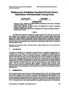
This operation as well as structurally analogous arithmetic operations for computing the log likelihood at the root of the tree and for optimizing the branch lengths in RAxML (and other ML-based inference programs) largely dominate execution times (approximately 90%). A fine-grain parallelization of Equation 1 is straight-forward because ~ (k) (c), L ~ (k) (c + 1) for site the likelihood vector entries L patterns c and c + 1 can be computed independently and thus simultaneously. Note that, P (bi ) and P (bj ) remain constant over all site patterns c = 1...m, where m is the number of site patterns in the partition that evolves according to the instantaneous nucleotide substitution model Q for time dt. To obtain P (bi ) for instance, we need to exponentiate Q by computing P (bi ) = eQbi via a standard eigenvector/eigenvalue decomposition. As long as we do not change the values in Q, the eigenvectors and eigenvalues of Q will not change. However, as we traverse a tree for evaluating it, we still need to compute P (b) = eQb for every branch and every partition of the dataset. Also note that, the matrix exponentiation must be conducted prior to computing ~ (k) (c) for all c. The cost of computing P (b) the entries in L is relatively small compared to the operations in Equation 1 when the number of site patterns m is large. However, when m is small, that is, there are only a few site patterns that evolve under a model Q, matrix exponentiation can dominate run times. Let us consider a simple example as outlined in Figure 1 with two cores c0 , c1 , and an alignment with two partitions p0 , p1 and two site patterns per partition. If we use a cyclic distribution of per-partition site patterns to cores, c0 will conduct likelihood operations on one site of partition p0 and one site of partition p1 . The same holds true for c1 . Because the dataset is partitioned, p0 will evolve under a model of nucleotide substitution Q0 and p1 under a model Q1 . Thus, if we use a cyclic per-partition site pattern distribution, each core will have to carry out a total of 4 matrix exponentiations for Q0 and Q1 to compute Equation 1. If we distribute the partitions monolithically to c0 and c1 , then c0 will only need to exponentiate Q0 and c1 only Q1 . Note that, especially for the distributed memory parallelization of Equation 1, it is not desirable to have each MPI process compute some P matrices and subsequently gather them (as needed) via a MPI collective communication operation. By using a monolithic partition-to-process assignment, we can avoid deploying an additional collective communication (or a barrier in the PThreads code) altogether, between the matrix exponentiations and the likelihood computations in Equation 1. Thus, if the number of partitions p is much larger than the number of cores n, our objective is to assign an approximately equal number of site patterns to each core and to distribute partitions monolithically to cores for amortizing the cost for Q matrix exponentiations. Ideally, we also

sites 0 & 1 evolve according to model Q0

p1

Q1 sites 2 & 3 evolve according to model Q1

0 1 2 3

cyclic distribution of sites

P(Q0) P(Q1)

11 00 0 1 00 11 0 1 00 11 0 1 00 11 0 1 0 2

core 0

P(Q0) P(Q1)

11 00 00 11 00 11 00 11 00 11 00 11 00 11 00 11 1 3

core 1

monolithic distribution of partitions

P(Q0)

111 0 00 0 1 00 011 1 00 11 011 1 00 0 1

core 0

P(Q1)

0111 00 101011 00 00 11 1011 00 2 3

core 1

Figure 1. Example for cyclic and monolithic distribution of sites and partitions to cores for a simple alignment with four sites and two partitions.

want each core to conduct an equal number of matrix exponentiations, that is, we want to balance the number of sites and partitions per core. IV. PARTITION S CHEDULING A LGORITHMS As already mentioned the current production-level implementation of RAxML-Light that is available via https: //github.com/stamatak/RAxML-Light-1.0.5 implements the simple and fast LPT heuristics. The monolithic per-partition data distribution to cores/MPI processes can be invoked via the -Q command line flag. If -Q is not specified, the parallel PThreads and MPI versions of RAxML-Light will use the standard cyclic per-partition distribution of site patterns to cores. In addition to LPT, we also implemented three slightly modified standard heuristics and a dedicated algorithm that also tries to balance the number of partitions per core (and not only the number of sites). Henceforth, we consistently use phylogenetic terminology for describing the algorithms, that is, partitions instead of jobs and number of site patterns instead of job length. A. Standard Heuristics Improved 0/1 interchange (iZO): The 0/1 interchange algorithm by Fin and Horwowitz [10] comprises two steps: The first step initialize the n cores by randomly placing p partitions on them. In the second step, one partition will be moved from the most loaded core to the least loaded core if the makespan can be decreased. These interchanges are applied iteratively until makespan can not be further improved. 2 The worst-case performance of this approach is 2 − n+1 . The improved 0/1 interchange heuristics [17] simply use LPT for the first step instead of random assignments. Hence, the makespan of this improved 0/1 interchange method can never exceed that of LPT. It can be demonstrated that, the improved 0/1 interchange has the same worst-case ratio as LPT. Modified 3-PHASE (mTP): The 3-PHASE algorithm [13] —as the name suggests— consists of three phases: (i) the initialization phase, (ii) the job interchange

phase, and (iii) the job exchange phase. The job interchange number of partitions and the corresponding number of phase is similar to the 0/1 interchanges algorithm. However, accumulated site patterns Smin . Note that, Mmin and Pn it uses the trivial lower makespan bound C = i=1 Ci /n Mmax do not need to have been assigned the largest for guiding job reassignments, which can potentially generand smallest number of site patterns. Scan all partitions ate better results. Finally, the job exchange phase attempts Pi with Si sites that have been assigned to Mmax . If to exchange jobs between pairs of cores to further reduce Smin + Si ≤ M , then assign Pi to Mmin . Repeat step the makespan. To yield the two algorithms (3-PHASE versus 2 until no further improvement can be made. iZO) more comparable, we adapted the initialization phase Step 3: Find the core Mmax which has the largest number of of 3-PHASE to also use LPT. Note that, these modified 3partitions and Smax accumulated site patterns. For all PHASE heuristics can not perform worse than the improved the other cores Mj has Sj sites, scan all partitions Pi 0/1 interchange. with Si sites on Mmax , if Sj + Si ≤ M , then reassign Improved MultiFit (iMF): The MultiFit method [11] is Pi to Mj and go to step 2; else the algorithm terminate. inspired by a bin-packing method. It uses a bisection search V. E XPERIMENTAL S ETUP & R ESULTS for the minimal bin capacity Cmin such that all p partitions can be fit into n bins (cores). Then, for each detected A. Experimental Setup capacity, the First Fit Decreasing (FFD) [11] method is We generated simulated alignments to assess performance used to assign the partitions to the bins. As LPT, the FFD of the new data distribution scheme and the heuristics method requires all partitions to be sorted in descending described in Section IV. To emulate a realistic partition order according to the number of site patterns. The main length distribution, we extracted the gene lengths from the difference is that, FFD will then (after sorting) subsequently human protein reference sequence database (ftp://ftp.ncbi. assign the partitions to the core with the lowest index that sapiens/mRNA Prot/). The distribution of nih.gov/refseq/H can complete the job within the capacity Cmin , instead of human protein sequences lengths (corresponding to partition assigning the partition to the core with the least number lengths in ours experiments) is provided in Figure 2. of site patterns (LPT). This difference in the assignment We applied INDELible [19] to four distinct tree topolostrategy can generate a large variation in the number of gies with 10 taxa each to simulate two protein and two partitions that are assigned to each core. The bisection search DNA datasets. The properties of the simulated datasets are will search Cmin between the upper bound max(Pmax , 2C) summarized in Table I. The test datasets together with the and the lower bound max(P Pn max , C), where Pmax is the source code that implements various scheduling algorithms largest partition, and C = i=1 Ci /n. MultiFit has a worst11 −k in RAxML-Light can be downloaded at www.exelixis-lab. where k is the number of case performance of 9 + 2 org/Scheduling online material.zip. Note that, for our perexecuted bisection searches. Improved MultiFit (iMF) [18] formance assessment it does not matter if we use simulated deploys tighter bounds to improve the efficiency of the or real data, as long as the partition length distribution is algorithm. iMF first runs LPT to determine the makespan realistic. M . If M ≥ 1.5C then it stops, otherwise it will execute standard MultiFit with an initial upper bound of M and a Table I M lower bound of max( 4 − T EST DATA SET SIZES 1 , Pmax , C). 3

3n

B. Dedicated Heuristics The algorithms described so far are designed to minimize the makespan, as given by the number of accumulated site patterns per core. Since, on top of this, we desire each core to also be assigned an equal number of monolithic partitions (see Section III), we developed additional heuristics of our own. We introduce the vIC (interchange of jobs to minimize job number variance) method that strives to decrease the variance in the number of partitions per core, and at the same time strives not to increase the makespan. The vIC method consists of three steps: Step 1: Execute one of the standard multiprocessor algorithms to obtain an initial partition-to-core assignment and calculate the makespan M . Step 2: Find the core Mmax that has the largest number of partitions with the number of accumulated site patterns Smax . Also find the core Mmin which has the smallest

Test data set Protein 1 Protein 2 DNA 1 DNA 2

100 partitions 58032aa 50621aa 146875nt 153802nt

200 partitions 106984aa 110827aa 336755nt 333170nt

500 partitions 273578aa 290336aa 882494nt 876077nt

800 partitions 445940aa 437574aa 1342040nt 1288862nt

1000 partitions 570970aa 521612aa 1744252nt 1646677nt

Tests were run on an Infiniband-connected cluster at the Heidelberg Institute for Theoretical Studies that is equipped with 50 48-core AMD Magny-Cours nodes and 128GB of RAM each. We executed runs with the PThreads and MPIbased version of RAxML-Light on 24, 48, and 96 cores. B. Experimental Results The evaluation of the alternative scheduling algorithms was based on two values: makespan (maximum accumulated number of sites assigned to a core) and the variance of the number of partitions among cores. Both values should ideally be minimized. We measured RAxML-Light execution times for the standard implementation with a cyclic data

Table II M AKESPAN (M), VARIANCE (VAR ), VARIANCE OF V IC (VAR - V IC), EXECUTION TIMES UNDER GAMMA ( T-G) AND EXECUTION TIMES UNDER CAT ( T-C) IN SECONDS FOR 4 SCHEDULING ALGORITHMS AND THE STANDARD CYCLIC DATA DISTRIBUTION ON 24, 48, AND 96 CORES . T HE VAR COLUMN SHOWS THE JOB NUMBER VARIANCE OF THE SCHEDULING ALGORITHMS THAT DO NOT USE V IC IMPROVEMENT. T HE NEXT COLUMN (VAR - V IC) SHOWS THE VARIANCE IMPROVEMENT ( IF ANY ) OBTAINED BY APPLYING V IC. T HE NUMBER OF PARTITIONS VARIES FROM 100 TO 1000. T HE RUNS ON 24 AND 48 CORES WERE EXECUTED USING THE PT HREADS VERSION , RUNS ON 96 CORES RUNS WERE TESTED USING THE MPI VERSION ON DATA SETS WITH 1000 PARTITIONS ONLY. Protein 1 n p 24 100 200 500 800 1000 48 100 200 500 800 1000 96 100 200 500 800 1000 Protein 2 24 100 200 500 800 1000 48 100 200 500 800 1000 96 100 200 500 800 1000 DNA 1 24 100 200 500 800 1000 48 100 200 500 800 1000 96 100 200 500 800 1000 DNA 2 24 100 200 500 800 1000 48 100 200 500 800 1000 96 100 200 500 800 1000

M 2268 2931 7441 12046 15125 2268 1802 3746 6019 10118 2268 1802 2624 3026 10118 2138 4143 10647 16120 19274 2138 2483 5326 8062 9666 2138 2483 3830 4067 4855 3287 7123 18851 28812 36950 2816 6050 9462 14397 18529 2816 6050 5261 7261 16429 3584 7295 19498 29095 36771 2452 5512 9806 14549 18411 2452 5512 5170 7358 9283

LPT Var 1.472 0.638 0.388 0.638 11.13 0.493 0.763 0.659 0.430 9.263 0.039 0.493 0.789 1.034 1.847 LPT 1.222 0.472 0.472 0.388 0.222 0.534 1.138 0.951 0.388 0.305 0.039 0.597 1.581 0.951 0.701 LPT 0.555 1.138 0.305 0.222 2.638 0.576 1.013 0.659 0.388 4.388 0.039 0.472 1.164 0.868 1.305 LPT 0.305 0.805 0.305 0.472 0.222 0.368 0.763 0.409 0.388 0.138 0.039 0.513 0.560 0.638 0.472

/ iZO / mTP Var-vIC t-G 0.888 134 0.555 218 549 0.305 893 1113 0.118 128 0.388 121 0.618 288 466 8.597 668 0.097 0.519 1.180 581 / iZO / mTP 0.722 156 0.388 341 867 1328 1581 0.118 138 0.638 184 456 692 0.263 813 0.097 0.894 0.618 411 / iZO / mTP 87 385 0.138 2264 5587 2.555 9429 0.118 78 0.430 350 2176 0.347 5438 3.763 9225 0.097 0.727 0.722 1.180 8878 / iZO / mTP 96 0.722 381 2269 0.388 5418 8863 0.159 85 0.388 347 2177 0.305 5277 8682 0.097 0.394 0.555 0.430 8398

t-C 41 76 190 309 402 39 40 103 167 219 179

M 2268 2907 7430 12015 15107 2268 1802 3718 6011 10118 2268 1802 2624 3009 10118

Var 13.97 25.80 197.2 586.7 1010 0.493 10.34 47.99 140.5 457.9 0.039 0.493 26.20 33.68 1.847

49 111 304 441 551 43 57 155 235 292 180

2138 4091 10603 16089 19260 2138 2483 5307 8048 9631 2138 2483 3830 4026 4819

9.638 28.97 283.3 647.7 940.8 0.534 10.63 69.70 154.8 239.2 0.039 0.597 31.97 37.53 58.18

75 373 2161 5638 9289 74 367 2125 5581 9199 8921

3229 7099 18756 28735 36856 2816 6050 9382 14381 18432 2816 6050 5261 7192 16429

6.055 24.72 175.9 501.7 839.8 0.576 1.013 42.28 121.2 207.6 0.039 0.472 13.12 29.18 1.305

94 354 2186 5897 8754 92 348 2150 5848 8696 8463

3470 7219 19433 29004 36729 2452 5512 9727 14505 18368 2452 5512 5170 7262 9189

3.972 25.47 172.5 426.5 782.2 3.076 0.763 40.99 107.2 190.8 0.039 0.513 10.43 24.65 45.86

iMF Var-vIC 0.888

570.6 0.118 1.347 46.28 138.5 47.38 0.097 1.456 32.72 1.180 iMF 2.388 27.80 276.9 628.9 934.6 0.118 1.722 64.61 235.8 0.097 2.081 34.15 52.43 iMF 4.722 163.1 493.6 800.4 0.118 0.430 40.95 199.1 0.097 3.644 28.18 1.180 iMF 2.638 23.80 422.2 0.159 0.388 38.32

0.097 4.269 22.86 44.57

t-G 144 218 554 903 1127 128 136 291 473 750 585

t-C 43 100 270 435 565 38 42 144 239 250 179

161 341 878 1338 1598 139 209 457 715 830 423

51 136 389 575 730 43 63 208 324 417 230

91 387 2285 5595 9455 78 350 2178 5441 9242 8878

76 375 2151 5670 9307 74 367 2131 5577 9209 8921

96 381 2269 5417 8887 90 347 2185 5283 8688 8412

95 353 2157 5904 8779 94 348 2152 5863 8708 8484

Standard t-G 179 349 881 1434 1779 129 264 654 1063 1313 1129 Standard 223 478 1216 1895 2306 158 334 845 1327 1627 1289 Standard 97 409 2335 5703 9559 84 367 2227 5547 9364 9051 Standard 105 400 2313 5496 8969 92 365 2236 5382 8795 8545

implementation t-C 303 616 1497 2393 3035 292 593 1443 2307 2920 2847 implementation 354 709 1783 2791 3512 338 673 1690 2668 3319 3319 implementation 99 457 2369 5978 9682 98 448 2345 5942 9641 9357 implementation 120 418 2341 6160 9077 119 411 2321 6141 9047 8962

100

2550

90

2500

LPT+vIC Standard implementation

80

Execution time in seconds

Number of occurrence

2450 70 60 50 40 30

2400 2350 2300 2250

20

2200

10

2150

0 0

1000

2000

3000

4000

5000

6000

7000

8000

9000

Protein sequences length (amino acid)

2100

0

4

8

12

16

20

24

28

32

36

40

44

48

Number of cores

Figure 2. Human protein sequences length distribution. Five proteins that are longer than 9000 amino acids are not shown in the histogram.

Figure 3. Execution times for 500 DNA data partitions under the CAT model (DNA 1).

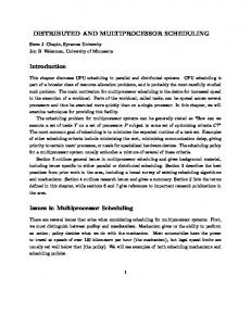
distribution strategy and the scheduling heuristics including vIC improvement. The results are depicted in Table II. Across all test configurations, LPT, iZO, and mTP returned identical results. This suggests that partition interchange and/or exchange as implemented in iZO and mTP does outperform LPT in our experiments. Generally, iMF yielded a smaller makespan, but at the cost of a substantially larger per-core partition number variance. When we applied vIC, the variance could be further reduced without increasing the makespan in most of the cases. Nonetheless, the iMF partition number variance is still much larger than for other algorithms, even after applying vIC to correct for this. As indicated by our results, the processing times for iMF-based data distribution is still longer than for alternative approaches, because of the high partition number variance and despite the fact that the makespan is smaller. With respect to absolute execution times, LPT (iZO and mTP) returned the best results. For one protein dataset (1000 partitions on 48 cores) under the CAT model of rate heterogeneity [20], we observed an 11-fold speedup with respect to the standard implementation. For protein data under the Γ model of rate heterogeneity [21] the average speedup is around two-fold. On the DNA datasets, we observe an average speedup of 1.386 under CAT model (see Figure 3) and 1.046 under Γ speed up. The main reason for the differences between DNA and protein data is that matrix exponentiation of the 20 × 20 Q matrix is substantially more expensive than for the 4 × 4 nucleotide substitution matrix. The difference between the CAT and Γ models of rate heterogeneity is due to the fact, that more Q matrix exponentiations are required per partition to obtain the transition probability matrices P for each persite rate category ri (for details please see [20]). Overall, the expected performance improvements depend on the ratio of

CPU cycles required for exponentiating the Q matrix and for computing Equation 1. The iMF-based partition distribution is always slower than LPT (iZO and mTP) because of the large variances. See, for instance, protein dataset 2 with 500 partitions on 24 cores where iMF returned a makespan of 10, 603 and LPT( iZO and mTP) a makespan of 10, 647 site patterns. However, the partition number variance of iMF is 276.9 compared to a variance of only 0.472 for LPT(iZO and mTP). Therefore, the iMF-based partition distribution is 28% slower than the LPT(iZO and mTP)-based approach under the CAT model of rate heterogeneity. With respect to parallel scalability, the standard implementation (cyclic distribution of sites) scales poorly above 4 cores, while the LPT(iZO and mTP)-based parallelization scales well, in particular on large protein data sets under the CAT model (see Figure 4). The simple LPT heuristics, return the best results in our test data. This is not only because it can distribute the processing time (number of site patterns) evenly among cores, but also because it assigns an approximately equal number of partitions to each core. Thus, each core calculates the likelihood vector entries on approximately the same number of site patterns and computes roughly the same number of P matrices. iMultifit did not perform well, despite the fact that it can distribute the sites more evenly among cores than LPT. This is because iMultifit assigns few large partitions to cores with the lower index number, and many, small partitions to cores with higher index numbers. Therefore, cores with higher index numbers need to calculate many more P matrices such that the load balance actually becomes worse. Hence, more elaborate heuristics than LPT, did not substantially improve the makespan. This may be due to the distribution of human gene lengths we sampled from to obtain partition lengths and the limited number of data

40

With respect to future work, we intend to integrate a mechanism in RAxML that will automatically and adaptively determine whether cyclic or monolithic scheduling shall be deployed. Moreover, we will work on fine-tuning and further optimizing load balance by allowing for a mix of cyclic as well as monolithic data distribution of sites/partitions to cores. The problems that we will encounter in this context are similar to the multi-processor scheduling problem with preemption.

LPT+vIC Standard implementation

36 32

Speedup

28 24 20 16 12

ACKNOWLEDGMENT 8 4 0

0

4

8

12

16

20

24

28

32

36

40

44

48

Number of cores

Figure 4. Speedup of LPT+vIC over the standard implementation (cyclic distribution of sites) for 1000 protein data partitions under the CAT model (Protein dataset 2).

sets we tested. One may expect more elaborate heuristics to improve the makespan when there is a large number of very small jobs. However, one important result from our study is that, the simple LPT heuristics that are easy to implement already yield substantial performance improvements. In general, multiprocessor scheduling algorithms for partitions should be used and implemented for cases where p  n. In cases where the largestPpartitions is greater than n the average completion time C = i=1 Ci /n, the makespan will be dominated by this partition and the code will hence not scale well. One such example is the protein dataset 1 with 100 partitions. VI. C ONCLUSION & F UTURE W ORK To the best of our knowledge, this paper is the first to describe the analogy of the multi-processor scheduling problem to load balance issues in large parallel partitioned phylogenetic analyses. Essentially, the phylogenetic scheduling/data distribution problem represents a bi-criterion problem, since the number of sites and partitions assigned to each core needs to be balanced. We show that, the simple and fast-to-compute LPT heuristics work well for solving the load balance problem. LPT has already been integrated into the production-level version of RAxML-Light. Moreover, we show that, parallel execution times can be improved by up to one order of magnitude for partitioned protein datasets under the CAT model of rate heterogeneity when partitions are distributed monolithically to cores using LPT. The techniques we have developed and assessed here, can be generally applied to all likelihood function implementations (Bayesian and Maximum Likelihood inference) that exploit the intrinsic parallelism of the PLF at a fine-grain level.

Part of this work was supported by the Graduate School for Computing in Medicine and Life Sciences funded by Germanys Excellence Initiative (DFG GSC 235/1) and by a visiting PhD student scholarship of the Heidelberg Institute for Theoretical Studies. R EFERENCES [1] J. Felsenstein, “Evolutionary trees from DNA sequences: a maximum likelihood approach,” J. Mol. Evol., vol. 17, pp. 368–376, 1981. [2] M. Ott, J. Zola, A. Stamatakis, and S. Aluru, “Large-scale maximum likelihood-based phylogenetic analysis on the ibm bluegene/l,” in Proceedings of the 2007 ACM/IEEE conference on Supercomputing. ACM, 2007, p. 4. [3] A. Stamatakis and M. Ott, “Exploiting fine-grained parallelism in the phylogenetic likelihood function with mpi, pthreads, and openmp: A performance study,” Pattern Recognition in Bioinformatics, pp. 424–435, 2008. [4] D. L. Ayres, A. Darling, D. J. Zwickl, P. Beerli, M. T. Holder, P. O. Lewis, J. P. Huelsenbeck, F. Ronquist, D. L. Swofford, M. P. Cummings, A. Rambaut, and M. A. Suchard, “Beagle: an application programming interface and high-performance computing library for statistical phylogenetics,” Systematic Biology, 2011. [5] R. Graham, E. Lawler, J. Lenstra, and A. Kan, “Optimization and approximation in deterministic sequencing and scheduling: a survey,” Annals of discrete Mathematics, vol. 5, no. 2, pp. 287–326, 1979. [6] D. Johnson and M. Garey, “Computers and intractability: A guide to the theory of np-completeness,” Freeman&Co, San Francisco, 1979. [7] M. DellAmico and S. Martello, “Optimal scheduling of tasks on identical parallel processors,” ORSA Journal on Computing, vol. 7, no. 2, pp. 191–200, 1995. [8] E. Mokotoff, “An exact algorithm for the identical parallel machine scheduling problem,” European Journal of Operational Research, vol. 152, no. 3, pp. 758–769, 2004. [9] R. Graham, “Bounds for certain multiprocessing anomalies,” Bell System Technical Journal, vol. 45, no. 9, pp. 1563–1581, 1966.

[10] G. Finn and E. Horowitz, “A linear time approximation algorithm for multiprocessor scheduling,” BIT Numerical Mathematics, vol. 19, no. 3, pp. 312–320, 1979.

[16] A. Stamatakis and M. Ott, “Load balance in the phylogenetic likelihood kernel,” in Parallel Processing, 2009. ICPP’09. International Conference on. IEEE, 2009, pp. 348–355.

[11] E. Coffman Jr., M. Garey, and D. Johnson, “An application of bin-packing to multiprocessor scheduling,” SIAM Journal on Computing, vol. 7, pp. 1–17, 1978.

[17] M. Langston, “Improved 0/1-interchange scheduling,” BIT Numerical Mathematics, vol. 22, no. 3, pp. 282–290, 1982.

[12] M. Gualtieri, P. Pietramala, and F. Rossi, “Heuristic algorithms for scheduling jobs on identical parallel machines via measures of spread,” IAENG International Journal of Applied Mathematics, vol. 39, 2009. [13] G. Paletta and F. Vocaturo, “A composite algorithm for multiprocessor scheduling,” Journal of Heuristics, vol. 17, no. 3, pp. 281–301, 2011. [14] L. Tang and J. Luo, “A new ils algorithm for parallel machine scheduling problems,” Journal of Intelligent Manufacturing, vol. 17, no. 5, pp. 609–619, 2006. [15] E. Hou, R. Hong, and N. Ansari, “Efficient multiprocessor scheduling based on genetic algorithms,” in Industrial Electronics Society, 1990. IECON’90., 16th Annual Conference of IEEE. IEEE, 1990, pp. 1239–1243.

[18] C. Lee and J. David Massey, “Multiprocessor scheduling: combining lpt and multifit,” Discrete applied mathematics, vol. 20, no. 3, pp. 233–242, 1988. [19] W. Fletcher and Z. Yang, “Indelible: a flexible simulator of biological sequence evolution,” Molecular biology and evolution, vol. 26, no. 8, pp. 1879–1888, 2009. [20] A. Stamatakis, “Phylogenetic models of rate heterogeneity: a high performance computing perspective,” in Parallel and Distributed Processing Symposium, 2006. IPDPS 2006. 20th International. Ieee, 2006, pp. 8–pp. [21] Z. Yang, “Maximum likelihood phylogenetic estimation from DNA sequences with variable rates over sites,” J. Mol. Evol., vol. 39, pp. 306–314, 1994.