The Robstuness of Neural Networks for Modelling and ... - CiteSeerX
Recommend Documents
and do remarkably well outperforming all other models in a simple trading simulation ... Christian Dunis is Professor of Banking and Finance at Liverpool Business School and ..... Our trading strategy applied is simple: go or stay long when the.
ABSTRACT. An experimental solar steam generator, consisting of a parabolic trough collector, a high pressure steam circulation circuit, and a suitable flash ...
economical damages caused by inundations. ... During high flows episodes, the spatial and temporal distribution of the rainfall field rules ...... List of Figures. 1.
Sep 3, 2014 - with the School of Computer Science, University of Nottingham, Jubilee. Campus ... noise, high dimensionality and the presence of outliers and.
Mar 30, 2012 - definition as described in (1). Here the system input â output relationship does not include the time component (2). Ym (Xn) = f(Xn, Pu). (2).
Neural networks are commonly used for classification and regression. The Bayesian approach may be employed, but choosing a prior for the parameters ...
postcript accesible vÃa Internet, http://www.itm.hk-r.se/~akear/bursty.html ... [5] Leland, W.E., Taqqu, M.S., Willinger, W., y Wilson, D.V. âOn the self-similar nature ...
P.O. Box 118, S â 221 00 Lund Sweden ... I would like to express my gratitude to all the people who has helped me to carry out this work. ...... List of Figures.
Avinash Kumar Agarwal, (2007). Biofuels (alcohols and biodiesel) applications as fuels for internal combustion engines,Progress in Energy and Combustion ...
Mar 2, 2011 - Robo is a numerical code specifically designed to study the evolution of the ISM. It includes several atomic and molecular species linked ...
Oct 1, 1997 - used to convert the output level of a unit into a signal that acts like a weight ...... by comparison to some actively held template as part of the processing of the frontal ... users/nn/lateral-interaction-book/cover.html. Alexander, G
Approximating and Simulating the Stochastic Growth Model: Parameterized Expectations, Neural Networks, and the Genetic Algorithm. John Duffy. Department ...
contribute to neglect symptoms, both in monkeys (Gaffan & Hornak, 1997) and in humans. (Doricchi ... (Chokron et al., 2004; Mark et al., 1988). Importantly ...
A particularly successful algorithm is the cascade-correlation architecture 6]. It begins with a minimal network with no hidden units, then automatically trains and ...
governor of turbogenerators on multimachine power systems. The neurocontroller ... stationary, fast acting, multi-input-multi-output (MIMO) device with a wide ...
generation was the slide-rule, where products and divisions were very efficiently done by adding and subtracting logarithms graphically represented on the rule!
Feb 10, 2018 - Four state-of-the-art machine learning algorithms are used for the ...... [19] Beale, M.H., Hagan, M.T., Demuth, H.B.: Neural Network Toolboxâ¢.
which is located to the north of Adelaide, South Australia. A 5-year data set containing ... dosing rate at the Hope Valley water treatment plant, South Australia.
bUnited Water International Pty Ltd, Adelaide, Australia. Abstract: ... which is located to the north of Adelaide, South Australia. ..... Nevada City, 1994. Maier, H. R. ...
University of Sunderland, School of. Computing, Engineering ... different training methodologies for the Autoassociative neural network are presented in detail.
is empirically investigated with a constructivist neural network model of the acquisi- ... that are released and taken up by neurons in the central nervous system.
of both information about objects and movements may be called situation model. Here, we ..... These networks are used to represent the real world situation.
important information related to the brain activity. A specific gene from the ... Authorized licensed use limited to: Auckland University of Technology. Downloaded on .... input has its own weight j;s-j"wr and E, Inn.ma,-~-n (r), i.e.. ' We employed
The Robstuness of Neural Networks for Modelling and ... - CiteSeerX
providers and on the ECB's website shortly after the concentration procedure has been .... Moving Average of the EUR/USD exchange rate return. 15. 11.
The Robstuness of Neural Networks for Modelling and Trading the EUR/USD Exchange Rate at the ECB Fixing by Christian L. Dunis* Jason Laws* Georgios Sermpinis* ( *Liverpool Business School, CIBEF Liverpool John Moores University) JEL Classification:C45
November 2008
Abstract The motivation for this paper is to investigate the use, the stability and the robustness of alternative novel neural network architectures when applied to the task of forecasting and trading the Euro/Dollar (EUR/USD) exchange rate using the European Central Bank (ECB) fixing series with only autoregressive terms as inputs. This is done by benchmarking the forecasting performance of three different neural network designs representing a Higher Order Neural Network (HONN), a Recurrent Network (RNN) and the classic Multilayer Percepton (MLP) with some traditional techniques, either statistical such as a an autoregressive moving average model (ARMA), or technical such as a moving average concergence/divergence model (MACD), plus a naïve strategy. More specifically, the trading performance of all models is investigated in a forecast and trading simulation on the EUR/USD ECB fixing time series over the period January 1999-August 2008 using the last eight months for out-ofsample testing. Our results in terms of their robustness and stability are compared with a previous work of the authors who apply the same models and follow the same methodology forecasting the same series, using as out-ofsample the period from July 2006 to December 2007. As it turns out, the HONN and the MLP networks present a robust performance and do remarkably well outperforming all other models in a simple trading simulation exercise in both papers. Moreover, when transaction costs are considered and leverage is applied, the same networks continue to outperform all other neural network and traditional statistical models in terms of annualised return, a robust and stable result as it is identical to the one obtained from the authors in their previous work, studying a different period for the series. Keywords Higher Order Neural Networks, Recurrent Networks, Leverage, Multi-Layer Perceptron Networks, Quantitative Trading Strategies. ____________ Christian Dunis is Professor of Banking and Finance at Liverpool Business School and Director of the Centre for International Banking, Economics and Finance (CIBEF) at Liverpool John Moores University (E-mail: [email protected]). Jason Laws is Reader of Finance at Liverpool Business School and a member of CIBEF (Email: [email protected]). Georgios Sermpinis is an Associate Researcher with CIBEF (E-mail: [email protected]) and currently working on his PhD thesis at Liverpool Business School. CIBEF – Centre for International Banking, Economics and Finance, JMU, John Foster Building,98 Mount Pleasant, Liverpool L3 5UZ.
1
1. INTRODUCTION Neural networks are an emergent technology with an increasing number of real-world applications including Finance (Lisboa et al. (2000)). However their numerous limitations and the contradicting empirical evident around their forecasting power are often creating scepticism about their use among practitioners. The motivation for this paper is to investigate not only the use of several new neural networks techniques that try to overcome these limitations but also the stability and robustness of their performance. This is done by benchmarking three different neural network architectures representing a Multilayer Percepton (MLP), a Higher Order Neural Network (HONN) and a Recurrent Neural Network (RNN). Their trading performance on the Euro/Dollar (EUR/USD) time series is investigated and is compared with some traditional statistical or technical methods such as an autoregressive moving average (ARMA) model or a moving average convergence/divergence (MACD) model, and a naïve strategy. In terms of the stability and robustness of our findings, we compare them with the conclusions of Dunis et al. (2008b) who apply the same models and follow the same methodology to forecast the same series, using however a different out-of-sample period. Concerning the inputs of our neural networks, we use the exact same selection of inputs and lags with Dunis et al. (2008b). Similarly, our MACD model is identical with the one of Dunis et al. (2008b) while on the other hand our ARMA model is different, as we need all coefficients to be significant in the new in-sample period. Moreover, our conclusions can supplement not only those of Dunis et al. (2008b) but also those of Dunis and Chen (2005) and Dunis and Williams (2002) who conduct similar forecasting competitions over the EUR/USD and the USD/JPY foreign exchange rates using about the same networks but with multivariate series as inputs. Concerning our data, the EUR/USD daily fixing is published by the European Central Bank (ECB) and is a tradable quantity as is possible to leave orders with a bank and trade on that basis. As it turns out, the MLP and HONN demonstrate a remarkable performance and outperform the other models in a simple trading simulation exercise. Moreover, when transaction costs are considered and leverage is applied the MLP and HONN models continue to outperform all other neural network and traditional statistical models in terms of annualised return. As these results are identical to those of Dunis et al. (2008b) who follow the same methodology but for a different period of the EUR/USD ECB fixing series, we can argue that the forecasting superiority of the HONN and the MLP is stable and robust over time. In terms of the RNN, their poor performance in this research may be due to their inability to provide good enough results when only autoregressive terms are used as inputs. The rest of the paper is organised as follows. In section 2, we present the literature relevant to the Recurrent Networks and the Higher Order Neural Networks. Section 3 describes the dataset used for this research and its characteristics. An overview of the different neural network models and statistical techniques is given in section 4. Section 5 gives the empirical results 2
of all the models considered and investigates the possibility of improving their performance with the application of leverage. In that section we also test the robustness of our models. Section 6 provides some concluding remarks.
2. LITERATURE REVIEW The motivation for this paper is to apply some of the most promising new neural networks architectures which have been developed recently with the purpose to overcome the numerous limitations of the more classic neural architectures and to assess whether they can achieve a higher performance in a trading simulation using only autoregressive series as inputs. RNNs have an activation feedback which embodies short-term memory allowing them to learn extremely complex temporal patterns. Their superiority against feedfoward networks when performing nonlinear time series prediction is well documented in Connor and Atlas (1993) and Adam et al. (1994). In financial applications, Kamijo and Tanigawa (1990) applied them successfully to the recognition of stock patterns of the Tokyo stock exchange while Tenti (1996) achieved good results using RNNs to forecast the exchange rate of the Deutsche Mark. Tino et al. (2001) use them to trade successfully the volatility of the DAX and the FTSE 100 using straddles while Dunis and Huang (2002), using continuous implied volatility data from the currency options market obtain remarkable good results for their GBP/USD and USD/JPY exchange rate volatility trading simulation. HONNs were first introduced by introduced by Giles and Maxwell (1987) as a fast learning network with increased learning capabilities. Although their function approximation superiority over the more traditional architectures is well documented in the literature (see among others Redding et al. (1993), Kosmatopoulos et al. (1995) and Psaltis et al. (1998)), their use in finance so far has been limited. This has changed when scientists started to investigate not only the benefits of Neural Networks (NNs) against the more traditional statistical techniques but also the differences between the different NN model architectures. Practical applications have now verified the theoretical advantages of HONNs by demonstrating their superior forecasting ability and put them in the front line of applied research in financial forecasting. For example Dunis et al. (2006b) use them to forecast successfully the gasoline crack spread while Fulcher et al. (2006) apply HONNs to forecast the AUD/USD exchange rate, achieving a 90% accuracy. However, Dunis et al. (2006a) show that, in the case of the futures spreads and for the period under review, the MLPs performed better compared with HONNs and recurrent neural networks. Moreover, Dunis et al. (2008a), who also study the EUR/USD series for a period of 10 years demonstrate that when multivariate series are used as inputs the HONNs, RNN and MLP networks have a similar forecasting power. Finally, Dunis et al. (2008b) in a paper with a methodology identical to that used in this research, demonstrate that HONN and the MLP networks are superior in forecasting the EUR/USD ECB fixing until the end of 2007, compared to the RNN networks, an ARMA model, a MACD and a naïve strategy.
3
3. THE EUR/USD EXCHANGE RATE AND RELATED FINANCIAL DATA The European Central Bank (ECB) publishes a daily fixing for selected EUR exchange rates: these reference mid-rates are based on a daily concentration procedure between central banks within and outside the European System of Central Banks, which normally takes place at 2.15 p.m. ECB time. The reference exchange rates are published both by electronic market information providers and on the ECB's website shortly after the concentration procedure has been completed. Although only a reference rate, many financial institutions are ready to trade at the EUR fixing and it is therefore possible to leave orders with a bank for business to be transacted at this level. The ECB daily fixing of the EUR/USD is therefore a tradable level which makes our application more realistic1. Name of period
Trading days 2474 2304 170
Total dataset In-sample dataset Out-of-sample dataset [Validation set]
Beginning End 4 January 1999 29 August 2008 4 January 1999 31 December 2007 2 January 2008 29 August 2008
Table 1: The EUR/USD dataset
4/7/2008
4/1/2008
4/7/2007
4/1/2007
4/7/2006
4/1/2006
4/7/2005
4/1/2005
4/7/2004
4/1/2004
4/7/2003
4/1/2003
4/7/2002
4/1/2002
4/7/2001
4/1/2001
4/7/2000
4/1/2000
4/7/1999
1.7 1.6 1.5 1.4 1.3 1.2 1.1 1 0.9 0.8 4/1/1999
EUR/USD
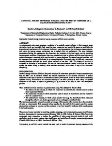
The graph below shows the total dataset for the EUR/USD and its upward trend since early 2006.
The observed EUR/USD time series is non-normal (Jarque-Bera statistics confirm this at the 99% confidence interval) containing slight skewness and high kurtosis. It is also nonstationary and hence we decided to transform the
1
The EUR/USD is quoted as the number of USD per Euro: for example, a value of 1.2657 is USD1.2657 per 1 Euro. We examine the EUR/USD since its first trading day on 4 January 1999, and until 29 August 2008.
4
EUR/USD series into a stationary daily series of rates of return2 using the formula:
P Rt = t − 1 Pt −1
[1]
Where Rt is the rate of return and Pt is the price level at time t. The summary statistics of the EUR/USD returns series reveal a slight skewness and high kurtosis. The Jarque-Bera statistic confirms again that the EUR/USD series is non-normal at the 99% confidence interval. 500 Series: RETURNS Sample 1 2473 Observations 2473
400
Mean Median Maximum Minimum Std. Dev. Skewness Kurtosis
Fig. 2: EUR/USD returns summary statistics (total dataset) As inputs to our networks and based on the autocorrelation function and some ARMA experiments we selected a set of autoregressive and moving average terms of the EUR/USD exchange rate returns and the 1-day Riskmetrics volatility series. Number 1 2 3 4 5 6 7 8 9 10 11 12
Variable EUR/USD exchange rate return EUR/USD exchange rate return EUR/USD exchange rate return EUR/USD exchange rate return EUR/USD exchange rate return EUR/USD exchange rate return EUR/USD exchange rate return EUR/USD exchange rate return EUR/USD exchange rate return Moving Average of the EUR/USD exchange rate return Moving Average of the EUR/USD exchange rate return
Lag 1 2 3 7 11 12 14 15 16 15 20
1-day Riskmetrics Volatility
1
Table 2: Explanatory variables In order to train our neural networks we further divided our dataset as follows: 2
Confirmation of its stationary property is obtained at the 1% significance level by both the Augmented Dickey Fuller (ADF) and Phillips-Perron (PP) test statistics.
5
Name of period Trading days Total data set 2474 Training data set 1794 Test data set 510 Out-of-sample data set [Validation set] 170
Beginning 4 January 1999 4 January 1999 2 January 2006 2 January 2008
End 29 August 2008 31 December 2005 31 December 2007 29 August 2008
Table 3: The neural networks datasets
4. FORECASTING MODELS 4.1 Benchmark Models In this paper, we benchmark our neural network models with 3 traditional strategies, namely an autoregressive moving average model (ARMA), a moving average convergence/divergence technical model (MACD) and a naïve strategy. 4.1.1 Naïve strategy The naïve strategy simply takes the most recent period change as the best prediction of the future change, i.e. a simple random walk. The model is defined by:
Yˆt +1 = Yt where
Yt Yˆ
t +1
[2]
is the actual rate of return at period t is the forecast rate of return for the next period
The performance of the strategy is evaluated in terms of trading performance via a simulated trading strategy. 4.1.2 Moving Average The moving average model is defined as: Mt =
(Yt + Yt −1 + Yt −2 + ... + Yt −n+1 ) n
[3]
where
Mt is the moving average at time t n is the number of terms in the moving average Yt is the actual rate of return at period t The MACD strategy used is quite simple. Two moving average series are created with different moving average lengths. The decision rule for taking positions in the market is straightforward. Positions are taken if the moving averages intersect. If the short-term moving average intersects the long-term moving average from below a ‘long’ position is taken. Conversely, if the longterm moving average is intersected from above a ‘short’ position is taken3.
The forecaster must use judgement when determining the number of periods n on which to base the moving averages. The combination that performed best over the in-sample subperiod was retained for out-of-sample evaluation. The 3
A ‘long’ EUR/USD position means buying Euros at the current price, while a ‘short’ position means selling Euros at the current price.
6
model selected was a combination of the EUR/USD and its 24-day moving average, namely n = 1 and 24 respectively or a (1,24) combination. The performance of this strategy is evaluated solely in terms of trading performance. 4.1.3 ARMA Model Autoregressive moving average models (ARMA) assume that the value of a time series depends on its previous values (the autoregressive component) and on previous residual values (the moving average component)4. The ARMA model takes the form: Yt = φ 0 + φ1Yt −1 + φ 2Yt −2 + ... + φ pYt − p + ε t − w1ε t −1 − w2ε t − 2 − ... − wq ε t − q
where
Yt Yt −1 , Yt − 2 , and Yt − p
[4]
is the dependent variable at time t are the lagged dependent variable
φ 0 , φ1 , φ 2 , and φ p εt ε t −1 , ε t −2 , and ε t − p
are regression coefficients
w1 , w2 , and wq
are weights.
is the residual term are previous values of the residual
Using as a guide the correlogram in the training and the test subperiods we have chosen a restricted ARMA (11,11) model. All of its coefficients are significant at the 95% confidence interval. The null hypothesis that all coefficients (except the constant) are not significantly different from zero is rejected at the 95% confidence interval (see Appendix A1). The selected ARMA model takes the form:
Yt = 12.8 ⋅ 10 −5 − 1.217Yt −1 − 0.478Yt − 2 − 0.140Yt − 7 + 0.197Yt −11 + 1.214ε t −1 + 0.474ε t − 2 + 0.152ε t − 7 − 0.218ε t −11
[5]
The model selected was retained for out-of-sample estimation. The performance of the strategy is evaluated in terms of trading performance.
4.1.4 Empirical Results for the Benchmark Models A summary of the empirical results of the 3 benchmark models on the validation subset is presented in the table below. The empirical results of the models in the training subperiod are presented in Appendix A.3 while Appendix A.2 documents the performance measures.
4
For a full discussion of the procedure, refer to Box et al.(1994) or Pindyck and Rubinfield (1998).
7
Sharpe Ratio Annualised Volatility Annualised Return Maximum Drawdown Positions Taken
Table 4: Trading performance of the benchmark models out-of-sample As can been seen the naïve strategy outperforms all other models by far. These results are surprising not only because the simplicity of the naïve model but also based on the training subperiod results (see Appendix A.3). There the naïve strategy presents an annualised return of -1.07% and a Sharpe ratio of 0.10. Moreover, with a closer look over the returns in our out-of-sample period we observe that the positive and the negative returns are clustered. In order to verify that the sequence of signs of the returns in the validation period is not random, we conduct the Wald-Wolfowitz or runs test for randomness5. The test confirms that the sequence of signs is not random at the 99% and 95% confidence interval. So as the naïve strategy is only using as a forecast for tomorrow today’s return, it is able to exploit this phenomenon and present a remarkable performance. This anomaly was not present in previous years and that is why the performance of the naïve strategy in-sample is so much worse. In the circumstances, this phenomenon is accidental and we have no reasons to believe that it should continue in the future and we thus discard the results of the naïve strategy from our conclusions.
4.2 Neural Networks Neural networks exist in several forms in the literature. The most popular architecture is the Multi-Layer Perceptron (MLP). A standard neural network has at least three layers. The first layer is called the input layer (the number of its nodes corresponds to the number of explanatory variables). The last layer is called the output layer (the number of its nodes corresponds to the number of response variables). An intermediary layer of nodes, the hidden layer, separates the input from the output layer. Its number of nodes defines the amount of complexity the model is capable of fitting. In addition, the input and hidden layer contain an extra node, called the bias node. This node has a fixed value of one and has the same function as the intercept in traditional regression models. Normally, each node of one layer has connections to all the other nodes of the next layer. The network processes information as follows: the input nodes contain the value of the explanatory variables. Since each node connection represents a weight factor, the information reaches a single hidden layer node as the weighted sum of its inputs. Each node of the hidden layer passes the information through a nonlinear activation function and passes it on to the output layer if the calculated value is above a threshold. The training of the network (which is the adjustment of its weights in the way that the network maps the input value of the training data to the corresponding 5
For a complete description of the test see Wald and Wolfowitz (1940).
8
output value) starts with randomly chosen weights and proceeds by applying a learning algorithm called backpropagation of errors6 (Shapiro (2000)). The learning algorithm simply tries to find those weights which minimize an error function (normally the sum of all squared differences between target and actual values). Since networks with sufficient hidden nodes are able to learn the training data (as well as their outliers and their noise) by heart, it is crucial to stop the training procedure at the right time to prevent overfitting (this is called ‘early stopping’). This can be achieved by dividing the dataset into 3 subsets respectively called the training and test sets used for simulating the data currently available to fit and tune the model and the validation set used for simulating future values. The network parameters are then estimated by fitting the training data using the above mentioned iterative procedure (backpropagation of errors). The iteration length is optimised by maximising the forecasting accuracy for the test dataset. Our networks, which are specially designed for financial purposes, will stop training when the profit of our forecasts in the test subperiod is maximized. Then the predictive value of the model is evaluated applying it to the validation dataset (out-of-sample dataset).
4.2.1 THE MULTI-LAYER PERCEPTRON MODEL 4.2.1.1 The MLP network architecture The network architecture of a ‘standard’ MLP looks as presented in figure 37: xt[k ]
ht[ j ]
~ yt
wj u jk
MLP
Fig. 3: A single output, fully connected MLP model where: [n] xt (n = 1,2,L, k + 1) are the model inputs (including the input bias node) at time t [m] ht (m = 1,2,..., j + 1) are the hidden nodes outputs (including the hidden bias node) ~ yt is the MLP model output u jk and w j are the network weights 6
Backpropagation networks are the most common multi-layer networks and are the most commonly used type in financial time series forecasting (Kaastra and Boyd (1996)). 7 The bias nodes are not shown here for the sake of simplicity.
9
is the transfer sigmoid function: S ( x ) = is a linear function: F ( x ) = ∑ xi
1 , 1 + e−x
[6] [7]
i
The error function to be minimised is: E (u jk , w j ) =
1 T (yt − ~yt (u jk , w j ))2 , with yt being the target value ∑ T t =1
4.2.1.2
Empirical results of the MLP model
[8]
The trading performance of the MLP on the validation subset is presented in the table below. We chose the network with the highest profit in the training subperiod. Our trading strategy applied is simple: go or stay long when the forecast return is above zero and go or stay short when the forecast return is below zero. Appendix A.3 provides the performance of the MLP in the training subperiod while Appendix A.4 provides the characteristics of our network. The results of other models are included for comparison.
Sharpe Ratio Annualised Volatility Annualised Return Maximum Drawdown Positions Taken
Table 5: Out-of-sample trading performance of the MLP As it can be seen the MLP outperforms our benchmark statistical models.
4.2.2 THE RECURRENT NETWORK Our next model is the recurrent neural network. While a complete explanation of RNN models is beyond the scope of this paper, we present below a brief explanation of the significant differences between RNN and MLP architectures. For an exact specification of the recurrent network, see Elman (1990). A simple recurrent network has activation feedback, which embodies short-term memory. The advantages of using recurrent networks over feedforward networks, for modelling non-linear time series, has been well documented in the past. However as described in Tenti (1996) “the main disadvantage of RNNs is that they require substantially more connections, and more memory in simulation, than standard backpropagation networks” (p.569), thus resulting in a substantial increase in computational time. However having said this RNNs
10
can yield better results in comparison to simple MLPs due to the additional memory inputs.
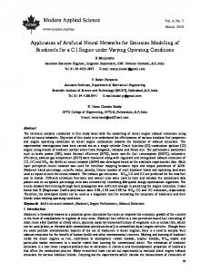
4.2.2.1 The RNN architecture A simple illustration of the architecture of an Elman RNN is presented below.
xj
[1]
xj
[ 2]
xj
[ 3]
Uj
~y
[1]
U j −1
[1]
Uj
t
[ 2]
[ 2]
U j −1
Fig. 4: Elman Recurrent neural network architecture with two nodes on the hidden layer. where:
xt
[n ]
[1] [2] (n = 1,2,L, k + 1) , ut , ut
~ yt
dt
[f]
Ut
[f]
( f = 1,2) and wt ( f = 1,2)
[n ]
are the model inputs (including the input bias node) at time t
is the recurrent model output (n = 1,2,L, k + 1) are the network weights is the output of the hidden nodes at time t 1 , 1 + e−x
is the transfer sigmoid function: S ( x ) = is the linear output function:
F (x ) = ∑ xi
[9]
[10]
i
The error function to be minimised is: E (d t , wt ) =
11
1 T ( yt − ~yt (dt , wt ))2 ∑ T t =1
[11]
In short, the RNN architecture can provide more accurate outputs because the [1] and inputs are potentially taken from all previous values (see inputs U j −1 [2]
U j−1 in the figure above). 4.2.2.2 Empirical results of the RNN model The RNNs are trained with gradient descent as were the MLPs. However, the increase in the number of weights, as mentioned before, makes the training process extremely slow taking ten times as long as the MLP. We follow the same methodology as we did for the MLPs for the selection of our optimal network. The characteristics of the network that we use are in Appendix A.4 while is a summary of the performance of the network in the training subperiod is given in Appendix A.3. The trading strategy is that followed for the MLP. As shown in table 6 below, the RNN has a worse performance compared to the MLP model when measured by the Sharpe ratio and annualised return. The results of other models are included for comparison.
Sharpe Ratio Annualised Volatility Annualised Return Maximum Drawdown Positions Taken
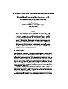
Table 6: Out-of-sample trading performance results of the RNN 4.2.3 THE HIGHER ORDER NEURAL NETWORK Higher Order Neural Networks (HONNs) were first introduced by Giles and Maxwell (1987) and were called “Tensor Networks”. Although the extent of their use in finance has so far been limited, Knowles et al. (2005) show that, with shorter computational times and limited input variables, “the best HONN models show a profit increase over the MLP of around 8%” on the EUR/USD time series (p. 7). For Zhang et al. (2002), a significant advantage of HONNs is that “HONN models are able to provide some rationale for the simulations they produce and thus can be regarded as “open box” rather then “black box”. Moreover, HONNs are able to simulate higher frequency, higher order nonlinear data, and consequently provide superior simulations compared to those produced by ANNs (Artificial Neural Networks)” (p. 188). 4.2.3.1 The HONN Architecture While they have already experienced some success in the field of pattern recognition and associative recall8, HONNs have not yet been widely used in finance. The architecture of a three input second order HONN is shown below: 8
Associative recall is the act of associating two seemingly unrelated entities, such as smell and colour. For more information see Karayiannis et al. (1994).
12
Fig. 5: Left, MLP with three inputs and two hidden nodes; right, second order HONN with three inputs where: [n ] xt (n = 1,2,L, k + 1) are the model inputs (including the input bias node) at time t ~ yt is the HONNs model output u jk are the network weights are the model inputs. is the transfer sigmoid function: S ( x ) = is a linear function:
1 , 1 + e−x
F (x ) = ∑ xi
[12]
[13]
i
The error function to be minimised is: E (u jk , w j ) =
1 T 2 ∑ (yt − ~yt (u jk ,)) , T t =1
with yt being the target value
[14]
HONNs use joint activation functions; this technique reduces the need to establish the relationships between inputs when training. Furthermore this reduces the number of free weights and means that HONNs are faster to train than even MLPs. However because the number of inputs can be very large for higher order architectures, orders of 4 and over are rarely used. Another advantage of the reduction of free weights means that the problems of overfitting and local optima affecting the results of neural networks can be largely avoided. For a complete description of HONNs see Knowles et al. (2005).
13
4.2.3.2 Empirical results of the HONN model We follow the same methodology as we did with RNNs and the MLPs for the selection of our optimal HONN. The trading strategy is that followed for the MLP. A summary of our findings is presented in table 7 below while Appendix A.3 provides the performance of the network in the training subperiod and Appendix A.4 provides its characteristics. The results of other models are included for comparison.
Sharpe Ratio Annualised Volatility Annualised Return Maximum Drawdown Positions Taken
Table 7: Out-of-sample trading performance results of the HONN We can see that the HONN performs significantly better than the RNN and the traditional MLP models.
5. TRADING COSTS, LEVERAGE AND ROBUSTNESS Up to now, we have presented the trading results of all our models without considering transaction costs. Since some of our models trade quite often, taking transaction costs into account might change the whole picture. We therefore introduce transaction costs as well as a leverage for each of our models. Moreover, we examine the robustness of our models by examining and comparing not only the results of our current research but also the conclusions of a previous research in which we studied the same series with the same models but over a different period. For comparability reasons we use the same selection of inputs for our NNs in both papers9. The only difference is the outof-sample period, here 2 January 2008 to 29 August 2008 while before we retained 3 July 2006 to 31 December 2007. The purpose of this test is to validate the robustness of our models through time and to provide concrete empirical evidence of the forecasting power of our models.
5.1
TRANSACTION COSTS
The transaction costs for a tradable amount, say USD 5-10 million, are about 1 pip (0.0001 EUR/USD) per trade (one way) between market makers. But as the EUR/USD time series considered here is a series of middle rates, the transaction cost is one spread per round trip. With an average exchange rate of EUR/USD of 1.532 for the out-of-sample period, a cost of 1 pip is equivalent to an average cost of 0.007% per position. In the table below we present the performance of our models after transaction costs are considered. 9
The complete paper Dunis et al. (2008b) is available at www.cibef.com.
14
Sharpe Ratio Annualised Volatility Annualised Return Maximum Drawdown Positions Taken Transaction Costs Annualised Return
Table 8: Out-of-sample trading performance results with transaction costs (02/01/08-29/08/08) We observe that although the HONN model presents higher transaction costs, it continues to outperform the other models in terms of annualised return. The MLP comes second while the RNN demonstrates a third best performance. On the other hand, the ARMA and MACD models have a rather disappointing performance as they both present negative annualised returns. Examining a different out-of-sample period, 3 July 2006 to 31 December 2007, but following the same methodology and using the same selection of inputs for our NNs, the results which are presented in the table below, were similar, only the MLP model outperformed the HONN in that out-of-sample period.
Sharpe Ratio Annualised Volatility Annualised Return Maximum Drawdown Positions Taken Transaction Costs Annualised Return
Table 9: Out-of-sample trading performance results with transaction costs (03/07/06-31/12/07) We observe that in both periods the MLP and HONN models clearly outperform the other strategies. In the latest period the HONN model has a better performance while one and a half year before the MLP presented better results. On the other hand, the ARMA model in both periods presents a rather disappointing trading performance. This empirical evidence allows us to argue that HONNs and MLPs have a consistent and better performance than the RNN, MACD and ARMA models in forecasting the ECB daily fixing of the EUR/USD.
5.3
Leverage to exploit low volatility
In order to further improve the trading performance of our models we introduce a “level of confidence” to our forecasts, i.e. a leverage based on the test subperiod that takes into account the low volatility of the trading performance of our models. For the ARMA and the MACD models, which show a negative return we do not apply leverage. The leverage factors applied are calculated in
15
such a way that each model has a common volatility of 10%10 on the test data set. The transaction costs are calculated by taking 0.007% per position into account, while the cost of leverage (interest payments for the additional capital) is calculated at 4% p.a. (that is 0.016% per trading day11). Our results are presented on the table 10 below.
Sharpe Ratio Annualised Volatility Annualised Return Maximum Drawdown Positions Taken Leverage Transaction Costs Annualised Return
Table 10: Trading performance - final results12 (02/01/08-29/08/08) As can be seen from the last row of table 10, the HONN model continues to demonstrate a superior trading performance. Similarly, the MLP and the RNN continue to perform well and present the second and the third highest annualised return respectively. In general, we observe that all models where leverage was applied were able to exploit it and increase their trading performance despite the higher transaction costs. The performance of our models for a different out-of-sample period, 3 July 2006 to 31 December 2007, is given in table 11 below.
Sharpe Ratio Annualised Volatility Annualised Return Maximum Drawdown Positions Taken Leverage Transaction Costs Annualised Return
Table 11: Trading performance - final results 12 (03/07/06-31/12/07)
10
Since most of the models have a volatility of about 10%, we have chosen this level as our basis. The leverage factors retained are given in table 11. 11 The interest costs are calculated by considering a 4% interest rate p.a. divided by 252 trading days. In reality, leverage costs also apply during non-trading days so that we should calculate the interest costs using 360 days per year. But for the sake of simplicity, we use the approximation of 252 trading days to spread the leverage costs of non-trading days equally over the trading days. This approximation prevents us from keeping track of how many nontrading days we hold a position. 12 Not taken into account the interest that could be earned during times where the capital is not traded (non-trading days) and could therefore be invested.
16
We note that in both periods the MLP and the HONN models continue to outperform the other models as they are able to exploit the leverage and present an increased trading performance in both out-of-sample periods. So even if the ranking of these two models is different in the two out-of-sample forecasting periods retained, they clearly outperform all other models in all cases something that allows us to argue with confidence about their forecasting superiority and their stability and robustness through time. On the other hand, the RNN model was not able to exploit the extra memory inputs in their architecture and presents rather disappointing results. Moreover, the time spent to derive the RNN results is ten times longer than the time needed with the HONN and the MLP models. Similarly, the MACD and the ARMA models present a very weak forecasting power even though their training subperiod performance was promising (see Appendix A.3).
6. CONCLUDING REMARKS In this paper, we apply Multi-layer Perceptron, Recurrent, and Higher Order neural networks to a one-day-ahead forecasting and trading task of the EUR/USD exchange rate using the European Central Bank (ECB) fixing series with only autoregressive terms as inputs. We use a naïve, a MACD and an ARMA model as benchmarks. Our aim is not only to examine the forecasting and trading performance of our models but also to see if this performance is stable and robust through time. In order to do so, we develop these different prediction models over the period January 1999 - December 2007 and validate their out-of-sample trading efficiency over the following period from January 2008 through August 2008. To examine the robustness and the stability of our models we compare our results with those from a previous research using the same models and the exact same selection of autoregressive terms as inputs to the neural networks, but with an out-of-sample period between July 2006 and December 2007. As it turns out, the MLP and HONN models clearly outperform the other models in both out-of-sample periods in terms of annualised return. Our conclusions are the same even after we introduced transaction costs and a leverage to exploit the low volatility of the trading performance of those models. This enables us to conclude with confidence over their forecasting superiority and their stability and robustness through time. On other hand, the RNN model seems to have a difficulty in providing good forecasts when only autoregressive series are used as inputs. Similarly, the ARMA and the MACD models present low or even negative annualised returns in this application despite their satisfactory training subperiod performance.
17
APPENDIX A.1 ARMA Model The output of the ARMA model used in this paper is presented below.
Dependent Variable: RETURNS Method: Least Squares Date: 09/03/08 Time: 17:28 Sample (adjusted): 12 2303 Included observations: 2292 after adjustments Convergence achieved after 59 iterations Backcast: ? 0 Variable
Coefficient
Std. Error
t-Statistic
Prob.
C AR(1) AR(2) AR(7) AR(11) MA(1) MA(2) MA(7) MA(11)
Mean dependent var S.D. dependent var Akaike info criterion Schwarz criterion F-statistic Prob(F-statistic) .65+.46i -.21-.82i -.94-.20i .66+.46i -.21+.83i -.94+.20i
A.4 Networks Characteristics We present below the characteristics of the networks with the best trading performance on the training subperiod for the different architectures.
REFERENCES Adam, O., Zarader, L. and Milgram, M. (1994), ‘Identification and Prediction of Non-Linear Models with Recurrent Neural Networks’, Laboratoire de Robotique de Paris. Box, G., Jenkins, G. and Gregory, G. (1994), Time Series Analysis: Forecasting and Control, Prentice-Hall, New Jersey. Connor, J. and Atlas, L. (1993), ‘Recurrent Neural Networks and Time Series Prediction’, Proceedings of the International Joint Conference on Neural Networks, 301-306. Dunis, C. and Huang, X. (2002), ‘Forecasting and Trading Currency Volatility: An Application of Recurrent Neural Regression and Model Combination’, Journal of Forecasting, 21, 5, 317-354. Dunis, C. and Williams, M. (2002), ‘Modelling and Trading the EUR/USD Exchange Rate: Do Neural Network Models Perform Better?’, Derivatives Use, Trading & Regulation, 8, 3, 211-239. Dunis, C. and Chen, Y. (2005), ‘Alternative Volatility Models for Risk Management and Trading: Application to the EUR/USD and USD/JPY Rates’, Derivatives Use, Trading & Regulation, 11, 2, 126-156. Dunis, C., Laws, J. and Evans B. (2006a), ‘Trading Futures Spreads: An application of Correlation and Threshold Filters’, Applied Financial Economics, 16, 1-12. Dunis, C., Laws, J. and Evans B. (2006b), ‘Modelling and Trading the Gasoline Crack Spread: A Non-Linear Story’, Derivatives Use, Trading & Regulation, 12, 126-145. Dunis, C., Laws, J. and Sermpinis, G. (2008a) ‘Higher Order and Recurrent Neural Architectures for Trading the EUR/USD Exchange Rate’, CIBEF Working Papers. Available at www.cibef.com. Dunis, C., Laws, J. and Sermpinis, G. (2008b) ‘Modelling and Trading the EUR/USD Exchange Rate at the ECB Fixing, CIBEF Working Papers. Available at www.cibef.com. Elman, J. L. (1990), ‘Finding Structure in Time’, Cognitive Science, 14, 179211. Fulcher, J., Zhang, M. and Xu, S. (2006), ‘The Application of Higher-Order Neural Networks to Financial Time Series’, Artificial Neural Networks in Finance and Manufacturing, Hershey, PA: Idea Group, London. Giles, L. and Maxwell, T. (1987) ‘Learning, Invariance and Generalization in Higher Order Neural Networks’, Applied Optics, 26, 4972-4978.
21
Kaastra, I. and Boyd, M. (1996), ‘Designing a Neural Network for Forecasting Financial and Economic Time Series’, Neurocomputing, 10, 215-236. Kamijo, K. and Tanigawa,T. (1990), ‘Stock Price Pattern Recognition: A Recurrent Neural Network Approach’, In Proceedings of the International Joint Conference on Neural Networks, 1215-1221. Karayiannis, N. and Venetsanopoulos, A. (1994), ‘On The Training and Performance of High-Order Neural Networks’, Mathematical Biosciences, 129, 143-168. Knowles, A., Hussein, A., Deredy, W., Lisboa, P. and Dunis, C. L. (2005), ‘Higher-Order Neural Networks with Bayesian Confidence Measure for Prediction of EUR/USD Exchange Rate’, CIBEF Working Papers. Available at www.cibef.com. Kosmatopoulos, E., Polycarpou, M., Christodoulou, M. and Ioannou, P. (1995), ‘High-Order Neural Network Structures for Identification of Dynamical Systems’, IEEE Transactions on Neural Networks, 6, 422-431. Lisboa, P. J. G. and Vellido, A. (2000), ‘Business Applications of Neural Networks’, vii-xxii, in P. J. G. Lisboa, B. Edisbury and A. Vellido [eds.] Business Applications of Neural Networks: The State-of-the-Art of Real-World Applications, World Scientific, Singapore. Pindyck, R. and Rubinfeld, D. (1998), Econometric Models and Economic Forecasts, 4th edition, McGraw-Hill, New York. Psaltis, D., Park, C. and Hong, J. (1988), ‘Higher Order Associative Memories and their Optical Implementations.’, Neural Networks, 1, 149-163. Redding, N., Kowalczyk, A. and Downs, T. (1993), ‘Constructive Higher-Order Network Algorithm that is Polynomial Time’, Neural Networks, 6, 997-1010. Shapiro, A. F. (2000), ‘A Hitchhiker’s Guide to the Techniques of Adaptive Nonlinear Models’, Insurance, Mathematics and Economics, 26, 119-132. Tenti, P. (1996), ‘Forecasting Foreign Exchange Rates Using Recurrent Neural Networks’, Applied Artificial Intelligence, 10, 567-581. Tino, P., Schittenkopf, C. and Doffner, G. (2001), ‘Financial Volatility Trading Using Recurrent Networks’, IEEE Transactions in Neural Networks, 12, 4, 865874. Wald, A. and Wolfowitz, J. (1940), "On a test whether two samples are from the same population," Annals of Mathematical Statistics, 11, 147-162.
22
Zhang, M., Xu, S., X. and Fulcher, J. (2002), ‘Neuron-Adaptive Higher Order Neural-Network Models for Automated Financial Data Modelling’, IEEE Transactions on Neural Networks,13,1, 188-204.