The shallow structure of a surface-rupturing fault in ...

Tectonophysics 717 (2017) 628–644

Contents lists available at ScienceDirect

Tectonophysics journal homepage: www.elsevier.com/locate/tecto

The shallow structure of a surface-rupturing fault in unconsolidated deposits from multi-scale electrical resistivity data: The 30 October 2016 Mw 6.5 central Italy earthquake case study Fabio Villani a,⁎, Vincenzo Sapia b a b

Istituto Nazionale di Geofisica e Vulcanologia, L'Aquila, Italy Istituto Nazionale di Geofisica e Vulcanologia, Rome, Italy

a r t i c l e

i n f o

Article history: Received 21 March 2017 Received in revised form 27 July 2017 Accepted 1 August 2017 Available online 03 August 2017 Keywords: Electrical resistivity tomography Surface faulting Fault imaging Fault zone properties Earthquake Central Apennines

a b s t r a c t We report the results of a shallow electrical resistivity investigation performed across a normal fault that ruptured the surface displacing with average ~0.05 m vertical offset alluvial fan deposits (b 23 kyr old) within an intermontane fault-bounded basin following the 30 October 2016 Mw 6.5 earthquake in central Italy. We adopted a multi-scale geophysical approach, by acquiring three 2-D electrical resistivity tomography (ERT) profiles centred on the coseismic ruptures, and characterized by different spatial resolution and investigation depth. Below the fault scarp, the ERT models show a narrow (~ 10 m wide) and steeply-dipping moderately-resistive region (100–150 Ωm), which we interpret as the electrical response of the fault zone displacing layers of relatively high-resistivity (300–700 Ωm) values. We explain the electrical signature of the retrieved fault zone as due to an increment of permeability caused by coseismic fracturing, and to the subsequent water migration from adjacent shallow aquifers squeezed by compaction induced by seismic waves. By using a statistically-based classification of electrical units, we estimate that the shallowest alluvial fan layer is affected by 2.7 ± 0.9 m vertical offset, which is consistent with the measured 2.3–2.8 m morphologic offset of the top fan surface, and suggesting a post-12 kyr throw-rate of 0.23 ± 0.08 mm/yr. Similarly, we evaluate a post-23 kyr throw of 5.1 ± 1.7 m, indicating a Late Pleistocene throw-rate of 0.22 ± 0.07 mm/yr, in accordance with available paleoseismic data. We further hypothesize a minimal total fault throw N 30 m, which likely accrued since the Middle Pleistocene (possibly in the last 350–500 kyr). The investigated fault structure is therefore an important splay characterized by a thick and highly permeable damage zone in unconsolidated deposits, and which ruptured the surface during several tens of strong (M N 6) earthquakes. © 2017 Elsevier B.V. All rights reserved.

1. Introduction Most of the strain affecting the upper crust in active extensional non-volcanic environments is accommodated by brittle normal fault zones (Sibson, 1977; Cowie and Scholz, 1992; Putz-Perrier and Sanderson, 2008). Fault zones often include one or more principal slip surfaces located within a fault core, where the largest displacement occurs, surrounded by a zone of fractured host rocks denoted as damage zone (Shipton et al., 2006). Large-displacement extensional faults are usually associated with damage zones whose width may attain tens of meters or even more, and which develop through time by shearing and mechanical crushing of wall-rocks during repeated episodes of coseismic slip (Agosta and Aydin, 2006). The geometry and physical properties of fault zones depend on the overall long-term fault structural evolution, including especially the ⁎ Corresponding author. E-mail address: [email protected] (F. Villani).

https://doi.org/10.1016/j.tecto.2017.08.001 0040-1951/© 2017 Elsevier B.V. All rights reserved.

processes of three-dimensional fault growth, the incremental accumulation of displacement, and the progressive localization of strain within one or multiple and relatively narrow principal shear zones (Walsh and Watterson, 1988; Cowie et al., 1995; Walsh et al., 2001; Childs et al., 2009). Analysis of fault populations has led to the recognition of scaling law relationships, showing that fault zone width generally increases with fault dimensions and displacement (Kim and Sanderson, 2005; Mitchell and Faulkner, 2009; Faulkner et al., 2011): the large scatter in the available datasets is usually interpreted in terms of dependence from the type of deformation elements that accommodate displacement, the protolith nature, the geometry of pre-existing structures and the mechanical stratigraphy involved in the process of fault growth (Shipton et al., 2006; Ferrill et al., 2017). The internal architecture of fault zones may be highly complex, since they typically display strong lithological heterogeneity, physical discontinuity and textural anisotropy. These properties are of primary importance in controlling underground fluid flow at different structural levels, from the very shallow subsurface down to seismogenic depths

F. Villani, V. Sapia / Tectonophysics 717 (2017) 628–644

(Gumundsson, 2000; Rawling et al., 2001; Henriksen and Braathen, 2005; Vincenzi et al. 2009; Masset and Loew, 2010). For instance, faults may act as barriers to fluid flow, or they may represent preferential pathways for migration of fluids. This quasi-static scenario becomes even more complex in the case of active faults, where a sealed damage zone behaving as a barrier during long inter-seismic periods may suddenly be breached when coseismic slip occurs, leading to rapid expulsion and diffusion of mixed-phase fluids in the surrounding volume (Caine et al. 1996; Townend and Zoback, 2000; Sibson, 2001). In this regard, fluids flow is crucial in the physical evolution of the damage zones, since it promotes chemical reactions that may lead to fault weakening due to development of low-friction clay-rich material, or conversely it can also contribute to healing by facilitating lithification of breccia and gauge (detailed review in: Faulkner et al., 2010). In general, only limited portions of active brittle fault zones are exposed at the surface, due to the combined result of erosion and tectonic rock exhumation. In many cases, active normal faults trigger rapid feedback response of surface processes, such as gravitational instability and erosional dismantling of the uplifted footwall blocks, coupled with enhanced sedimentation in the downthrown hangingwall counterpart (Bull, 2009; Burbank and Anderson, 2011). This results in a complex setting of the uppermost structural levels, particularly in the case of tectonically active regions characterized by low strain-rates and mountain environments typical of several upland regions in the Mediterranean area and in particular in the interior of peninsular Italy: here, distributed deformation on segmented normal fault-systems and the presence of thick clastic covers may hinder important details of the active fault structure, making it difficult to correctly decipher the signature of recent faulting (more details in: Villani et al., 2015a). For these reasons, geophysical investigation of active fault zones can provide unique insight (Everett, 2013). Electrical resistivity methods proved successful in imaging the subsurface of such complex structures (Suzuki et al., 2000; Caputo et al., 2003; Nguyen et al., 2005). It has long been recognized that many active faults, of different tectonic environments, are often characterized by lower electrical resistivity signatures with respect to the surrounding host rocks (Ritter et al., 2005). The main processes that lead to low electrical resistivity within fault zones are: 1) a higher degree of fracturing within the damage zone, which increases permeability thus facilitating fluid circulation; 2) the development of clayey minerals along the slip surfaces and within the damage zone; 3) reaction-driven changes in porosity of the protolith. Among the numerous examples worldwide, narrow zones of relatively low-resistivity have been detected across subsurface faults in the Basin and Range Province of Western United States (Park and Wernicke, 2003) and the San Andreas Fault (Unsworth et al., 1997; Park and Roberts, 2003; Unsworth and Bedrosian, 2004), in Japan (Electromagnetic Research Group for Active Fault, 1982), in France (Gélis et al., 2010), in Slovakia (Putiška et al., 2012), in Belgium (Lecocq and Camelbeeck, 2017) and in central-southern Italy (among the others: Giocoli et al., 2015 and references therein). In this study, we acquired 2-D electrical resistivity tomography data (ERT) through a multi-scale approach in order to image the shallow subsurface structure of an active normal fault zone in the epicentral area of the 30 October 2016 Mw 6.5 earthquake that hit central Italy (Fig. 1). As described in the following section, this strong earthquake caused primary surface faulting, which involved a complex network of normal fault segments. Most of these structural features have a clear geomorphic expression and directly expose bedrock fault planes in high and impervious mountainous areas. Our investigation is focused on one active strand that, despite its trace develops entirely within recent clastic deposits with a subtle morphological imprint, ruptured up to the surface during the 2016 seismic sequence. Our primary target is the recognition of the subsurface fault geometry and the width of the damage zone as inferred by its electrical resistivity signature, with relations to the style of recent faulting and the long-term tectonic activity. We define the main electrical units as recovered from the resistivity

629

sections in the very shallow subsurface, in relation to a pre-existing paleoseismological trench and available geological data. A rigorous statistical analysis yields to a quantitative classification of the overall resistivity data distribution and depth to layers. As a result, we argue on fault zone displacement and rupture geometry including also the possible role of fluids flow in the damage zone. We then discuss the broad geological implications of the obtained results. Worthy to note, this nearsurface, multi-scale geophysical investigation in a fault-controlled area was performed during a running seismic sequence, and the upcoming prohibitive winter conditions of this mountain region required the application of a fast and accurate shallow exploration of the subsurface soon after the occurrence of a destructive earthquake. 2. Geological background 2.1. Geology and seismotectonics of the central Apennines The study area (Fig. 1) is located in the axial portion of the central Apennines, a NE-verging fold-and-thrust belt developed since the Early-Middle Miocene by the overthrusting and stacking of mostly Meso-Cenozoic calcareous shallow-to-deep water and Miocene turbiditic domains belonging to the former passive Adria margin (Malinverno and Ryan, 1986; Patacca et al., 2008; Cosentino et al., 2010; Vezzani et al., 2010). The compressional front migrated towards the Adriatic side of the chain, where it is still active, while a generalized post-orogenic extension affects the westernmost and inner portions since the Late Pliocene – Early Pleistocene (Lavecchia et al., 1994; Cavinato and De Celles, 1999; Ghisetti and Vezzani, 1999; D'Agostino et al., 2001). The normal faults network dissecting the central Apennines axis consist of 5–10 km long, mostly NW-trending and SW-dipping, individual segments, forming complex systems up to 25–30 km long (Fig. 1; Galadini and Galli, 2000; Morewood and Roberts, 2000; Cowie and Roberts, 2001; Roberts et al., 2002, 2004; Tondi and Cello, 2003). Most of them show clear hints of recent activity, due to the offset of Quaternary continental deposits and the fresh exposure of bedrock fault planes, interpreted as mostly due to rapid exhumation during coseismic surface slip episodes occurring after the Last Glacial Maximum (Giraudi, 1995; Benedetti et al., 2013). Geologic and paleoseismic data covering the Late-Pleistocene-Holocene time interval (Galli et al., 2008) coupled with high-resolution geophysical investigations (e.g.: Villani et al., 2017) provide values of individual fault slip-rates in the 0.2–1.3 mm/yr range. The central Apennines are characterized by one of the highest seismic releases in the Mediterranean area, mostly due to shallow (~ 5– 15 km deep) crustal earthquakes of normal-faulting type and with magnitude M occasionally up to ~6.5–7, which occur within a ~50–80 kmwide and actively extending belt (Fig. 1) that parallels the topographic bulge of the chain (Chiarabba et al., 2005; Pondrelli et al., 2006; Chiarabba and Chiodini, 2013; see also updated database of moment tensor solutions available at http://cnt.rm.ingv.it/tdmt, and at http:// eqinfo.eas.slu.edu/eqc/eqc_mt/MECH.IT/). Furthermore, the current extensional regime is evidenced by borehole breakout analyses (Montone et al., 2012), and geodetic data, which provide regional extension rates in the range of ~ 1–2.5 mm/yr (Hustand et al. 2003; D'Agostino et al., 2008; Faure Walker et al., 2010; Devoti et al., 2011; Carafa et al., 2015). Clearly, there is an inextricable link between the current seismicity, the extension affecting the chain and the active normal faults network so far described. The study area is located along the easternmost active fault-system in the central Apennines, running ~ 30 km within the Sibillini Mts. Range (Calamita and Pizzi, 1992, 1994; Calamita et al., 1992; Cello et al., 1997; Pizzi et al., 2002; Mt. Vettore - Mt. Bove fault-system, VBFS for short, marked in red in Fig. 1). Equivalently, Lavecchia et al. (1994) interpret this fault-system as the breakaway zone of the active extensional domain in this part of the central Apennines. Before the summer of 2016, the background level of instrumental seismicity in the region

630


Fig. 1. Simplified structural sketch of the central Apennines (shaded relief topography from a 10-m DEM by Tarquini et al., 2012). The circles show all the M N 3 earthquakes recorded by the Italian Seismic Network between 1985 and December 2016 with hypocentral depth 0–15 km. The focal mechanisms of the main five events of the 2016 Amatrice-Norcia seismic sequence and of the 6 April 2009 Mw 6.1 L'Aquila earthquake are shown (data from: http://cnt.rm.ingv.it/tdmt; 1, Mw 6.0, 2016-08-24; 2, Mw 5.4, 2016–08-24, 3, Mw 5.4, 2016-10-26; 4, Mw 5.9, 2016-10-26; 5, Mw 6.5, 2016-10-30). The main Quaternary normal faults (black lines, tick on the downthrown side) and the Mt. Vettore – Mt. Bove fault system (VBFS: red lines, tick on the downthrown side) are indicated (compilation from the following works: Vezzani et al., 2010; Pierantoni et al., 2013). The yellow rectangle encloses the Pian Grande di Castelluccio shown in Fig. 2. (For interpretation of the references to colour in this figure legend, the reader is referred to the web version of this article.)

did not clearly highlight the seismic activity of the VBFS, as compared to nearby faults to the west (1979, Mw 5.9 Norcia earthquake; Deschamps et al., 1984) and to the north-west (1997, Mw 6.0 Colfiorito earthquake; Amato et al., 1998). Previous studies considered silent or locked the VBFS (Galadini and Galli, 2003; Boncio et al., 2004), because the

relatively low degree of seismicity and the lack of historical earthquakes was coupled to striking geomorphic evidence of post-Last Glacial Maximum (LGM) activity (Calamita et al., 1992; Calamita and Pizzi, 1994; Lavecchia et al., 1994) and hints of Holocene paleoseismicity (Galadini and Galli, 2000; Galli et al., 2008). For the VBFS, Pizzi et al. (2002)


evaluate a total geologic throw as large as 1200 m in the Mt. Bove sector (to the north) and 1350 m in the Mt. Vettore sector (to the south), whereas the estimated maximum Quaternary morphologic throw is on the order of 800 m. The strong seismic potential of the VBFS suddenly came out in 2016, when it triggered an important seismic sequence (details in: Chiaraluce et al., 2017). It begun on August the 24th 2016 at 1:36:32 UTC with an Mw 6.0 earthquake that caused heavy damage and 299 casualties, and located to the NW of Amatrice (8 km depth, #1 in Fig. 1; Gruppo di Lavoro INGV sul terremoto di Amatrice, 2016; Tinti et al., 2016). The mainshock was followed 1 h later by an Mw 5.4 event (8.7 km depth, #2 in Fig. 1). The sequence culminated with three other major shocks, occurring on October the 26th (Mw 5.4, 17:10:36 UTC, depth 9.3 km, #3 in Fig. 1; Mw 5.9, 19:18:05 UTC, depth 8.4 km, #4 in Fig. 1; Gruppo di Lavoro INGV sul Terremoto di Amatrice, 2016; Gruppo di Lavoro INGV sul Terremoto di Visso, 2016), and on October the 30th with epicenter close to Norcia (Mw 6.5, 6:40:17 UTC, depth 9.4 km, #5 in Fig. 1; Gruppo di Lavoro INGV sul Terremoto in Centro Italia, 2016). The last earthquake was the largest seismic event recorded in the past four decades in the Italian peninsula since the devastating Ms 6.9 1980 Campania-Basilicata earthquake (Westaway and Jackson, 1987; Bernard and Zollo, 1989). The 24 August earthquake provoked surface faulting, which was clearly observed for a minimal total length of about 5.2 km along the southernmost part of the VBFS, with average vertical displacement of nearly 0.10–0.15 m (EMERGEO Working Group, 2016; Pucci et al., 2017). The 26 October Mw 5.9 quake caused surface faulting as well in the northernmost part of the VBFS, however geologists did not have the time to complete field surveys before the 30 October earthquake occurred. This last event caused an impressive and complex pattern of surface faulting, which involved a complex system of SW-dipping and also NE-dipping faults segments whose southernmost part was already activated by the August quakes, for a total length of ~25 km: locally, vertical offset of the ground surface caused by primary surface faulting along limestone bedrock fault planes of the Mt. Vettore sector exceeded 1.5– 2 m (Gruppo di Lavoro INGV sul Terremoto in Centro Italia, 2016, 2017; Pantosti and the Open EMERGEO Working Group, 2017; Civico and the Open EMERGEO Working Group, submitted; Villani and the Open EMERGEO Working Group, in prep.). 2.2. Quaternary intermontane basins in the central Apennines and geophysical signature of the infilling deposits The long-term activity of the above mentioned Quaternary normal faults array in the central Apennines resulted in the generation of several intermontane basins (Cavinato and De Celles, 1999). Subsequent drainage incision due to large-scale regional uplift and normal blockfaulting in some cases led to the partial exposure of their continental infill, mostly made of lacustrine and fluvial/alluvial sequences, particularly in the basins located to the west of the present-day Apennines divide (D'Agostino et al., 2001; Bosi et al., 2003). However, only in a few cases a thorough investigation of the internal structure of these basins has been performed through the integration of geophysical and borehole data (see for instance: Cavinato et al., 2002). Recent research focused on the imaging of the intermontane tectonic basins close to the area struck by the 2009 Mw 6.1 L'Aquila earthquake (see Fig. 1 for location) took advantage of the extensive use of electrical and electromagnetic methods (Giocoli et al., 2011; Villani et al., 2015a, 2015b; Pucci et al., 2016; Porreca et al., 2016; Civico et al., 2017). In terms of electrical stratigraphy, these studies basically show that the alternation of roughly tabular bodies of contrasting resistivity fills in such continental depressions. For instance, in a wide area to the east of L'Aquila, recovered electrical resistivity models from Pucci et al. (2016) provide correlations between low-resistivity bodies (ρ b 20–50 Ωm) with known outcropping lacustrine marls and clays, and between moderately-to-high resistivity bodies (ρ N 100 Ωm) with mapped

631

carbonatic alluvial conglomerates. Similarly, in the same area, Villani et al. (2015a) established correlations between high-resistive bodies (ρ up to 500 Ωm) and stiff alluvial conglomerates, and between low-resistivity bodies (ρ b 80 Ωm) and sandy alluvial deposits containing sparse tephra. In the Piano di Pezza basin to the south of L'Aquila (PP in Fig. 1), Villani et al. (2015b) found good correlations between the electrical resistivity images and outcropping geology (very high-resistive moraines, characterized by ρ up to 3000 Ωm, and relatively low-resistive alluvial and colluvial deposits, with ρ b 200 Ωm). Moreover, based on the electrical resistivity results, these authors assume that the deeper sedimentary infill of the Piano di Pezza basin is characterized by a regular alternation of coarse-grained clastic deposits and gravels with silty-sandy matrix: this assumption was supported by the correlations with several boreholes stratigraphy from the nearby Campo Felice intermontane basin (CF in Fig. 1) as described by Giraudi et al. (2010), who recognized in the continental sequence the alternation of sands and gravels related to glacial and interglacial cycles in the last 0.5 Myr. Electrical resistivity surveys performed by several authors in the epicentral area of the 2009 L'Aquila earthquake, in many cases document shallow fault zones within gravelly and sandy deposits, and characterized by relatively low resistivity values (MS-AQ, 2010; Giocoli et al., 2011). In this regard, Villani et al. (2015b) show that the shallow subsurface portion of the Piano di Pezza normal fault disrupts gravels and sandy/silty colluvium, and depict a high-resolution geophysical image of the very shallow fault zone, being ≃7 m wide and characterized by very low P waves velocity (b750 m/s) and electrical resistivity (ρ b 200 Ωm) up to one order of magnitude lower than the surrounding coarse slope debris and moraine deposits (ρ N 2000 Ωm). 2.3. The survey site and the ancillary information The survey area is located in the Pian Grande di Castelluccio, a ≈7 km × 3 km wide intermontane basin developed in the hangingwall of the Mt. Vettore normal fault-system as result of the long-term subsidence of the downthrown fault blocks (Fig. 2; Calamita and Pizzi, 1992, 1994; Calamita et al., 1992). The almost flat-bottomed plain has an endoreic drainage, and displays a gentle dip to the south, with average elevations between 1330 and 1270 m a.s.l. It is surrounded by high and steep slopes on the western side and particularly on the eastern border, where the peaks of Mt. Vettore (2476 m) and Cima del Redentore (2448 m) represent the culminations of a N1100 m high cumulative fault scarp. The substratum is made of Jurassic to Paleogene shallow-to-deep marly-calcareous deposits, whereas the plain is filled with sequences of lacustrine, alluvial fan and fluvio-glacial deposits (Coltorti and Farabollini, 1995; Pierantoni et al., 2013). The main catchments conveying coarse sediments to the plain are located in the northern part, in the south-western sector and all along the western flank of the Mt. VettoreCima del Redentore ridge. Few shallow boreholes nearby the survey area are available (Ge.Mi.Na., 1963; Fig. 2 for location; details in Fig. 3). Two of these, very close to the basin borders, penetrated the pre-Quaternary marly limestones at 97 m and 80 m depth respectively, in the hangingwall of two NW-trending range-bounding faults. The overall stratigraphic data indicate the alternation of conglomerates, sandy gravels and clays with variable thickness as the result of the interfingering of alluvial fan and lacustrine deposits during the Quaternary. These data are used for calibration of the ERT resistivity models (see details in Section 4). Sparse vertical electrical resistivity soundings were acquired in the plain by Biella et al. (1981): their geophysical results, compared to borehole stratigraphy, indicate that gravels are characterized by ρ ≃ 140–220 Ωm, whereas sandy-clays have ρ ≃ 55–125 Ωm and the carbonatic substratum ρ N 1500 Ωm. The 30 October 2016 Mw 6.5 earthquake caused surface ruptures along this mountainside and also within the plain (Gruppo di Lavoro INGV sul Terremoto in Centro Italia, 2017; Civico and the Open

632


Fig. 2. Geological sketch of the Pian Grande di Castelluccio basin (modified and simplified after: Pierantoni et al., 2013). The blue rectangle encloses the survey site area shown in Fig. 4. The main fault strands of the VBFS that ruptured the surface during the 30 October 2016 Mw 6.5 earthquake are indicated in red, together with the Valle delle Fonti fault investigated in this work. (For interpretation of the references to colour in this figure legend, the reader is referred to the web version of this article.)

EMERGEO Working Group, submitted): here, they closely follow the trend of a subtle fault scarp affecting Late Pleistocene to Holocene alluvial fan deposits, and which was first recognized by Galadini and Galli (2003). The Authors explored the surficial portion of this fault scarp (which we label Valle delle Fonti fault) by means of three small paleoseismic trenches (details in Sections 3 and 4; Fig. 4), recovering a very shallow normal fault zone that displaces Holocene sandy and silty colluvial and alluvial deposits: they infer the occurrence of at least three major surface-rupturing paleo-earthquakes, one occurring between 4155-3965 years B.P. and the 6th–7th century CE, one between 5940-5890/5795–5780 years B.P. and 4155–3965 years B.P., and another one between 18.000-12.000 years B.P. and 5940– 5890/5795–5780 years B.P. 3. Data and methods 3.1. Geological and topographic data As members of the EMERGEO Working Group of the Istituto Nazionale di Geofisica e Vulcanologia, we carried out field surveys during fall 2016 to map the trace of the coseismic surface ruptures. Within the Pian Grande di Castelluccio we accurately reported, at closely spaced intervals, the height of the coseismic free face exposing recent soils (defining the coseismic fault throw) in addition to the opening of the

ground cracks (related to the local fault heave), with an intrinsic measurement error of ~0.01 m. Overall, we mapped N 1 km of almost continuous surface rupture, by collecting N 130 measurements (Fig. 4). These data are compared to the morphologic height of the cumulative fault scarp as revealed by serial topographic profiles, which we obtained by analyzing a 2-m grid DEM previously smoothed with a low-pass spatial filter in order to remove spikes. We also took into account the main sedimentary bodies within the plain as mapped by Coltorti and Farabollini (1995) and Galadini and Galli (2003). 3.2. Electrical resistivity data In order to recover the shallow subsurface electrical resistivity image of the fault zone, on December 2016 we investigated the subsoil over one transect (labelled A, Fig. 4) running WSW-ENE, and nearly orthogonal to the trace of the 30 October 2016 coseismic surface ruptures. Along this transect, we acquired three different scale-resolution 2-D ERT profiles using a Syscal R2 (IRIS Instrument) with a set of 64 stainless steel electrodes. All ERT profiles are purposely centred on the coseismic rupture and were acquired using an electrodes spacing of 2 m, 5 m and 10 m respectively, corresponding to profile lengths of 126 m, 315 m and 630 m (profiles P1_2m, P1_5m and P1_10m in Table 1). For each profile, we acquired both dipole-dipole (DD for short) and Wenner-Schlumberger (WS for short) electrode arrays, in order to 1)


633

the last iteration. The DD recordings proved a bit noisier, as expected, and yielded tomographic models with a higher RMS compared to WS data: this difference is more evident in the case of the ERT profile with 10 m electrodes spacing. Due to the larger investigation depth with respect to DD models, we show the average statistical properties of WS resistivity models by means of frequency histogram plots, in order to roughly discriminate the occurrence of different subsurface resistivity packages. 3.3. Interface classification

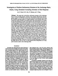
Fig. 3. Simplified stratigraphic columns of five boreholes within the Pian Grande di Castelluccio basin (modified after: Ge.Mi.Na., 1963). The colour scale (similar to that used for the ERT models) is assigned in order to qualitatively represent the average electrical resistivity response of each lithological unit (red-violet for resistive bodies and blue-green for conductive bodies). (For interpretation of the references to colour in this figure legend, the reader is referred to the web version of this article.)

reach different depths of investigation, 2) obtain a good compromise between vertical and horizontal resolution of the retrieved resistivity bodies (Loke and Barker, 1995; Table 1). With the DD configuration we aimed at better imaging lateral resistivity contrasts as due to faulting and/or abrupt horizontal changes in thickness of the sedimentary bodies. Conversely, with the WS configuration we aimed at confidently recovering both lateral and vertical resistivity contrasts while also increasing the depth of investigation beneath the coseismic rupture. We injected a square-wave signal for 250 ms into the ground, using 100, 200 and 400 Volts for the P1_2m, P1_5m, and P1_10m profiles, respectively. Resistance contact check allowed us to avoid relatively high resistance values. We used fresh water to enhance coupling between the electrodes and the ground. Although contact resistance is a known factor to impact on data quality, it is not the only one (LaBrecque et al., 1996). We used low voltage and high resistance contact records as noise indicators in the acquired ERT data. To account for noisy data, we manually edited obvious outliers and removed apparent resistivity data derived from very low voltage and/or current level before running the inversion. No weighting of data points in the inversion based on measurement errors was applied, since weighting by voltage or current “error” usually has very little effect in the inversion. Although being aware that a more suitable method to estimate such errors would be acquiring reciprocal records, we were not able to collect them with our instrument. Measured apparent resistivity data were input to a 2-D smoothnessconstrained least squares inversion algorithm, where the investigated subsurface area is subdivided into a mesh of rectangular blocks, whose width is equal to half of the electrode spacing in the shallowest layers (Constable et al. 1987; Loke and Dahlin, 2002). We then used a model discretization where layers thickness linearly increases by 10% with each incremental depth interval. In Section 4.2 we show the results obtained for linearized inversions with smoothness constraints. The quality of the obtained resistivity sections is then described by the root mean square (RMS) of residuals after

On each smooth ERT model (except for the noisier P1_10m DD recovered resistivity model) we classify the most significant resistivity changes as derived from the application of the steepest-gradient-method (SGM: Chambers et al., 2006; Sapia et al., 2017). Due to the expected roughly tabular and sub-horizontal subsurface stratigraphy of the survey site, in this work we applied a slightly modified SGM-based approach, described in more detail in the Auxiliary Material S1. The basic principle of the SGM is that the main interfaces are located in regions where a maximum increase or decrease in the resistivity at depth occurs, i.e. where the second derivative of a best-fit curve to a vertical array of resistivity data points (in this case, a polynomial curve) is null (Fig. S1). Our modified approach is based on the further condition of the third derivative of the polynomial-fit curve to be non-zero, in order to avoid saddle points. The input files are parsed to obtain regularly-spaced points, and the SGM is applied to each polynomial-fit curve along tens of vertical sections. We adopted the same approach to classify sub-vertical discontinuities by calculating the steepest gradient along horizontal sections: this was useful for corroborating the inferred location of subsurface faults. This method represents a semi-quantitative estimation to locate eventual subsurface discontinuities, which may aid in the stratigraphic and structural interpretation of tomographic images. 4. Results 4.1. Details of the coseismic surface rupture The outcropping geology of the survey site is characterized by a wide and polycyclic alluvial fan surface, which Galadini and Galli (2003) relate to five distinct phases of sedimentation characterized by a general southwards flow direction, and spanning the LGM-Holocene time interval (Valle delle Fonti alluvial fan, Fig. 2). We studied the morphology of the cumulative fault scarp affecting the most recent depositional body of the alluvial fan (comprising the 4th and 5th depositional phases of Galadini and Galli, 2003) by analyzing 28 topographic profiles (30–50 m spaced apart), about 100 m-long each, and running orthogonal to the average scarp trend (Fig. 4). We used the method by Bucknam and Anderson (1979) to derive the vertical separation of the alluvial fan top-surface on both sides of the scarp: since in this site the top-surface displays a gentle dip (typically b1%) towards the WSW, scarp height and vertical offset of the alluvial fan surface are nearly equal, and we use scarp height as a proxy for the local long-term morphologic throw of the fault. Fig. 5a shows some representative topographic profiles. The long-lasting agricultural activities in the area have in some cases heavily modified the original morphology of this tectonic landform, which only at places appears as a sharp step (e.g. profile 26 in Fig. 5a). The pictures in Fig. 5b and c show a closeup view of the 30 October 2016 surface rupture running at the base of the scarp, in the area of transect A. Fig. 6 shows the results of the morphological analysis. The blue curve is the envelope of the Valle delle Fonti fault scarp height values projected onto an 1120 m-long baseline parallel to the scarp trace. The average height of the scarp is ≃2.10 m. It exhibits an evident tapering at both ends, with three local maxima of ~2.80 m, 2.75 m and 2.70 m,

634


Fig. 4. Detail of the ERT survey site (Google Earth basemap). The detailed trace of the 30 October 2016 coseismic rupture is indicated with the red lines (tick on the downthrown side). The thin black lines indicate the topographic profiles discussed in the text, and the stars indicate the location of the paleoseismic trenches T1, T2 and T3 by Galadini and Galli (2003). (For interpretation of the references to colour in this figure legend, the reader is referred to the web version of this article.)

respectively from the north to the south (at site A the measured height is ~2.30 m). The red line in Fig. 6 is the envelope of the height of the 30 October 2016 surface rupture projected onto the same baseline used for the

Table 1 Details of the ERT profiles discussed in this paper. Profile

Length

Electrodes spacing

Array configuration

RMS

P1_2m P1_5m P1_10m

126 m 315 m 630 m

2m 5m 10 m

DD + WS DD + WS DD + WS

1.1% (DD); 0.9% (WS) 2.3% (DD); 0.64% (WS) 6.2% (DD); 3.1% (WS)

cumulative scarp. The style of the coseismic displacement is characterized by a vertical offset of the topographic surface with the western side down, frequently coupled with open cracks. Only in one limited portion (at approximately 400 m distance along the baseline in Fig. 6) we documented the occurrence of a couple of small counter-slope ruptures (eastern side down, vertical offset of 0.03–0.04 m). Overall, the average height of the coseismic free face is b0.06 m (median value 0.05 m), with three local maxima of 0.09 m, 0.12 m and 0.14 m that closely follow the maximum values of the cumulative scarp height. At site A (see also Fig. 5b and c), the 30 October 2016 surface rupture is characterized by a free face 0.11–0.12 m high, whereas crack opening locally reaches 0.05 m, even if in most places the coseismic displacement was accomplished by an exclusively vertical offset of the ground


635

Fig. 5. a) Selected topographic profiles across the cumulative Valle delle Fonti fault scarp (black bar is for vertical scale): the red arrows indicate the location of the 30 October 2016 coseismic rupture, and double arrows indicate the scarp height; b) close-up view of the coseismic rupture (white arrows) at the ERT survey site, looking towards the north (14 December 2016); c) close-up view of the coseismic rupture (white arrows) at the ERT survey site, looking towards the south (14 December 2016). Note the systematic small-scale en échelon structural pattern. (For interpretation of the references to colour in this figure legend, the reader is referred to the web version of this article.)

surface with no appreciable horizontal component. The opening of the coseismic ruptures also displays a systematic trend, with local maxima (between 0.04 and 0.06 m) closely following the peak values of the free face height. From a geometric point of view, the coseismic surface rupture is organized in about 15–16 smaller segments displaying a right-stepping geometry and a local variability in strike, with a mean trend of N169° in the southernmost part and N180° in the northernmost sector. Coseismic and long-term displacement curves have a very similar shape: the fact that the surface ruptures of 2016 follow closely the cumulative fault scarp suggests that the style of the 30 October 2016 rupture within the Pian Grande di Castelluccio is somewhat recurrent. Therefore, we choose the location of transect A where both peak coseismic and long-term morphologic offsets occur, in order to explore the portion of the fault that presumably accrued the largest cumulative displacement through time. We also took particular attention to be far enough the trench sites of Galadini and Galli (2003) in order to avoid any effect of backfilling and ground reworking on the subsurface resistivity structure.

4.2. ERT models Fig. 7 shows the inversion results for ERT profile P1_2m acquired with DD (panel a) and WS (panel b) arrays. Superimposed to the sections are the main interfaces as computed by the SGM method applied to the inverted resistivity data. We interpret different units characterized by comparable range of resistivity values and bounded by correlative interfaces as representative of distinct electrical resistivity intervals that we labelled with capital letters, in order to simplify the description of the resistivity sections. The western part of the ERTs exhibits a very shallow layer (unit A; b1 m thick on average) characterized by ρ b 170 Ωm, and locally being b100 Ωm: the bottom of this layer is defined by a sharp resistivity gradient. Unit A thickens towards the scarp and the related coseismic surface rupture, reaching a maximum of about 1.8 m at x = 62 m. Below unit A, both the western and eastern parts of the ERT models are characterized by a pack of high-resistivity material (ρ N 400 Ωm, unit B). Based on our classification method, unit B displays at places some additional internal and almost parallel interfaces, defining sub-

Fig. 6. Results of the morphological analysis. The blue line is the height of the cumulative Valle delle Fonti fault scarp projected onto an 1120 m-long baseline. The red line is the height of the 30 October 2016 coseismic free face, and the green line is the crack opening projected onto the same common baseline. The black arrow indicates the location of the ERT survey. (For interpretation of the references to colour in this figure legend, the reader is referred to the web version of this article.)

636


Fig. 7. a) ERT model for profile P1_2m in DD configuration; b) ERT model for profile P1_2m in WS configuration; c) frequency histogram of resistivity data for ERT model in WS configuration shown in panel b. The small black circles are interface points as inferred by the application of SGM along closely-spaced vertical profiles, and the small white circles on panel a represent sub-vertical belts of high resistivity gradient as inferred along horizontal profiles.

packages that we named B′ and B″, bearing in mind that they simply represent vertical resistivity changes within the same electrical unit B. Both models consistently show that the top of unit B′ displays different elevation to the west and to the east of the scarp (details in Section 5.2). Below the scarp, a relatively-low resistivity region (ρ ~100–170 Ωm) is evident at x = 60–66 m (unit FZ). The shape of this anomaly looks very similar in the overlapping part of both DD and WS models. The WS model further indicates that the lower part of this low-resistivity anomaly widens at depth, displaying a perceivable steep dip to the southwest. The frequency distribution of resistivity values for the WS model is shown in Fig. 7c (the bin size of 25 Ωm is used, based on the application of the Freedman-Diaconis rule; the same is applied for the other ERT models): it is characterized by three modes at ρ 125–150 Ωm, ρ 250– 300 Ωm, and ρ 425–500 Ωm, respectively. Whereas the two modes on the right well represent the resistive unit B, the low-resistivity mode is related mostly to unit FZ, and only the leftmost part of the histogram indicates the contribution of the thin unit A (ρ b 125 Ωm). The frequency distribution displays a marked asymmetry with a modal peak of high-resistivity (ρ 450–475 Ωm), since the shallower subsurface volume is prevalently characterized by resistive soils. Fig. 8 shows the inversion results of profile P1_5m for DD (panel a) and WS (panel b) arrays, respectively. Both models image in the western part below the shallow high-resistivity layer previously described (unit B) a N 12 m thick and nearly horizontal pack of relatively uniform low-resistivity (ρ b 130 Ωm), which we name unit C. This has no counterpart in the eastern part of both models, where a heterogeneous and patchy resistive body is found down to the bottom (ρ ~ 200–370 Ωm; unit D). As for results of profile ERT P1_2m, these models still image below the scarp a steeply-dipping and narrow zone of relatively low-resistivity (unit FZ), which displays some continuity with the easternmost

portion of unit C. The frequency distribution of resistivity for WS model of profile P1_5m is shown in Fig. 8c: it also displays three modes at 100– 125 Ωm, 275–325 Ωm, and 375–425 Ωm, respectively. With this array we sample a wider volume of the low-resistivity unit C, and we penetrate down to the deeper part of unit D-D′ (exhibiting a slight decrease of the resistivity downwards). Fig. 9 shows the inversion results of profile P1_10m for both DD (panel a) and WS (panel b) arrays. The overall pattern of the subsurface resistivity is consistent with results obtained for profile P1_5m. Data for array DD are quite noisy and the RMS residuals pretty high (Table 1), however the unit FZ is very clear, being 10–12 m wide, and it preserves a sub-vertical attitude down to the model bottom. Data for the WS array are of higher quality, and the obtained resistivity model suggests that unit FZ continues at depth (down to about 120 m below the ground surface) with comparable width and attitude. This model provides us with useful information at depth to definitely constrain the thickness of the low-resistivity unit C to about 25 m. It sheds lights on the depth extent of unit D, which turns to be about 40–42 m thick to the east of the scarp, overlying a low-resistivity region (ρ ~70–130 Ωm; unit E), about 50 m thick. Furthermore, the WS model indicates the presence of a high-resistivity region standing below unit C. Due to the roughly similar thickness and overall resistivity (ρ ~200–500 Ωm), we infer this body (unit D ′) may be equivalent to unit D. We acknowledge that some of the features at the bottom of the resistivity sections are characterized by low sensitivity, however the high-resistivity patch (ρ ~ 600–700 Ωm) in the lowermost part of model P1_10m WS is probably resolved, and it is quite in accordance with vertical resistivity soundings by Biella et al. (1981) suggesting that in this limited portion of the basin the pre-Quaternary carbonate basement is about 100–150 m deep. The frequency distribution of resistivity for WS model of profile P1_10m is shown in Fig. 9c: it displays two clear modes at ρ 150–225


637

Fig. 8. a) ERT model of profile P1_5m in DD configuration; b) ERT model of profile P1_2m in WS configuration; c) frequency plot of resistivity data from WS model. The small black circles are interface points as inferred by the application of SGM along closely-spaced vertical profiles, and the small white circles on panel a represent sub-vertical belts of high resistivity gradient as inferred along horizontal profiles.

Ωm and at ρ 400–450 Ωm, and a subordinate third mode at ρ 275–325 Ωm, respectively. This model hints to a deeper low-resistivity unit (E′) at the lower left corner of the resistivity section, although we are aware of the fact that the sensitivity at the bottom is significantly lower compared to the model resolution at the top. The frequency distribution is asymmetric and it is specular with respect to what found for profile P1_2m, since the lowermost portion of the investigated subsurface is characterized by low-resistivity soils. From the inspection of the histograms it follows that the unit FZ is difficult to discriminate based only on its resistivity, which is similar to units C and E. The main features of unit FZ are rather its sub-vertical shape and the marked continuity down to the bottom of the ERT models. 5. Discussion 5.1. Stratigraphic and structural interpretation of the ERT models For the stratigraphic interpretation of the shallow portion of the ERT models we rely on the paleoseismic trenches described by Galadini and Galli (2003) and on the few available boreholes (Fig. 2 and Fig. 3). Fig. 10 shows the projection of trench T1 with a simplified log over profile P1_2m (DD array). The trench revealed at the base of the scarp a sequence of silty deposits of alluvial and colluvial origin lying on sub-angular carbonate gravels, related to the alluvial fan. This setting is similar to what observed in the other two trenches. The thickness of the silty units ranges from b 1 m to about 1.7 m when crossing a complex normal fault zone, 4–5 m wide, and consisting of 6 to 11 small SW-dipping and subordinately NE-dipping splays (the number of splays varies in the three trenches). We observe a good correlation between the low-resistivity shallow unit A (ρ b 125 Ωm and 0.5–1.8 m thick) as recovered in profile

P1_2m at the base of the scarp and the colluvial-alluvial sandy-silty package recognized in the paleoseismic trenches by Galadini and Galli (2003). The age of unit A is well constrained by radiocarbon dating, and it spans the late Holocene (6005–1400 yr B.P.). The correlation between the shallowest portion of unit B and the alluvial fan gravels recovered in all the three trenches is straightforward. Therefore, carbonate gravels with a low amount of silty matrix are characterized by resistivity values in the range of 375–500 Ωm. The lithological nature of unit B is also confirmed by the closest borehole (#3 in Fig. 2 and Fig. 3) by Ge.Mi.Na. (1963). However, the age of this gravel deposit is less constrained, due to the lack of absolute dating. Galadini and Galli (2003) relate the growth of the complex alluvial fan of Valle delle Fonti to five different depositional phases ranging in age from the LGM (23–18 kyr B.P.) to about 3.8 kyr B.P.: this is based on the correlation with similar alluvial fan progradation phases recognized by Giraudi (1995) in some continental basins in the central Apennines to the south of the study area and sharing a comparable average elevation and geomorphic setting. More recent stratigraphic and geochronologic data from the Campo Felice area (CF in Fig. 1) by Giraudi et al. (2011) confirm the post-LGM age of these alluvial fan progradation events. The thickness of the shallowest part of unit B as recovered in our ERT models is about 2 m, and we infer that it represents the record of the two latest phases of alluvial fan accretion, 12–3.8 kyr B.P. in age. The borehole #5 in Fig. 2 is located at the westernmost edge of the outcropping alluvial fan of Valle delle Fonti, and it suggests that the thickness of the shallowest gravel unit is about 15 m. Similar thickness is also found in borehole #2 (20 m) and borehole #4 (17 m), which penetrate two smaller alluvial fans likely of the same age. These values are in accordance with results from ERT models P1_5m, which show that the overall thickness of unit B (including B′ and B″) is about 15 m. Assuming this chronologic framework is correct, we infer that unit B represents the electrical response of the overall alluvial fan of Valle delle Fonti,

638


Fig. 9. a) ERT model of profile P1_10m in DD configuration; b) ERT model of profile P1_10m in WS configuration; c) frequency plot of resistivity data from WS model. The small black circles are interface points as inferred by the application of SGM along closely-spaced vertical profiles, and the small white circles on panel b represent sub-vertical belts of high resistivity gradient as inferred along horizontal profiles.

spanning the last 23–3.8 kyr. The thickness of this alluvial fan requires a minimal long-term sedimentation rate of 0.65 mm/yr in the fault hangingwall. The low-resistivity unit C clearly visible in the resistivity models of profiles P1_5m and P1_10m is about 22–25 m thick. Unfortunately, borehole #5 does not show any fine-grained stratigraphical unit with comparable thickness, thus denoting a strong lateral variability of the

Fig. 10. Simplified log of Trench 1 from Galadini and Galli (2003) projected over the shallowest central portion of ERT model P1_2m DD (the outline of trench projected onto the ERT model is marked with grey dashed line). The solid black lines in the trench log are fault traces, whereas dashed black lines in the ERT model are inferred fault traces, which define the uppermost part of electrical unit FZ displacing unit B.

subsurface setting. However, boreholes #1 and #4 indicate the presence of a N20m thick layer of clays and silts at depth N 15 m, which may represent an equivalent of the conductive layer below the coarse deposits of the Valle delle Fonti alluvial fan. Therefore, we interpret unit C to be the electrical response of clay and silt with interbedded sandy gravels layers. The age of unit C is uncertain. A very crude age estimate is obtained by extrapolating the sedimentation rate of 0.65 mm/yr obtained for the uppermost unit B, resulting in 30–70 kyr B.P. Obviously, non-steady long-term sedimentation rates and the occurrence of unconformities would lead to a much older age for unit C. For instance, in the Campo Felice tectonic basin (CF in Fig. 1), Giraudi et al. (2011) document from borehole data five main cycles of lacustrine sedimentation in the hangingwall of the basin-bounding active normal fault: based on tephra chronology and pollen analyses, the authors interpret those cycles as depositional response to cold climatic phases, and in particular they relate to the marine isotope stages MIS6 and MIS4 (~191–57 ka) the 3rd and 4th cycles. The latter form a N 20 m thick pack of silts and sands whose top is ~20 m deep. Due to the comparable thickness and depth, we tentatively assign a similar age range to unit C, which we consider a lacustrine cycle developed during cold climatic conditions between the late Middle Pleistocene and before the LGM. The 30 m-thick unit D in the hangingwall of the fault (between 40 and 70 m depth) has no counterpart in the shallow borehole #5, although borehole #4 indicates the alternation of prevailing gravel and subordinate silt at comparable depth interval. We interpret unit D as a coarse-grained deposit, possibly related to old phases of alluvial fan accretion enhanced by colder climatic conditions, subsequently covered by the lacustrine deposits (unit C). In the fault footwall, the shallow resistive layer has a comparable thickness. Due to a relatively higher sedimentation rate in the hangingwall, we hypothesize that the resistive


layer in the footwall represents the condensed counterpart of units B, C and D. This may explain the absence of the conductive unit C to the east of the fault along the investigated transect. Conversely, we have hints of the presence of a deeper conductive unit (E and E′) on both sides of the fault. Possibly, unit E rests on the pre-Quaternary marly-calcareous basement at 110–120 m depth in the fault footwall (ERT model P1_10m). We have no means to date units D and E, however we infer they should be Middle Pleistocene in age (about 350–500 kyr old?), based on results for the Campo Felice basin by Giraudi et al. (2011), where they relate to the MIS 14 sandy gravel deposits in the 70–110 m depth range according to the absolute dating of interbedded tephra layers (~505 kyr old). 5.2. Fault zone geometry, displacement, and estimation of throw-rates The recognition of the main interfaces separating the electrical units as described in Section 4, and the chronologic framework discussed in Section 5.1, provide basic elements to infer the amount of cumulated fault throw and its rate. If we consider the average elevation of the nearly-horizontal base of the shallowest recognized resistive unit B (see ERT model P1_2m DD in Fig. 7) in the footwall and in the hangingwall of the fault, we get a vertical separation of 2.7 ± 0.9 m (Fig. 11). In the estimation of displacement we avoided to consider the top of unit B, because we do not have any means to evaluate the amount of erosion affecting the footwall block, moreover we disregarded points too close to the fault zone, since in this region the interfaces lose their sub-horizontal attitude. The obtained value is very close to the maximum cumulative morphologic offset of the Valle delle Fonti fault as inferred by the topographic analysis of the fault scarp (2.82 m; Fig. 5, Fig. 6), and a bit larger than the scarp height at the ERT survey site (~2.30 m). Due to the inherent smoothness of the resistivity models, we approximate that the morphologic and geologic offsets are nearly equal, and that they represent the fault throw occurred since the beginning of the sedimentation of the uppermost 2 m of the alluvial fan. Following the same approach, we evaluate the displacement affecting the base of the Valle delle Fonti alluvial fan (base of resistive unit B ″, according to results of ERT model P1_5m DD). Due to the complex geometry of the interfaces, in particular in the footwall block, the obtained value of 5.1 m ± 1.7 m is characterized by a larger standard error. However, it is indicative of an incremental fault offset affecting the deeper and older layers. Notably, the sequence B-B″ is about 8 m thick in the hangingwall and about 6 m thick in the footwall, thus confirming the syn-sedimentary activity of the investigated fault, causing higher sedimentation rates in the downthrown hangingwall block. We also note that the ERT transect is mostly orthogonal to the general flow direction of the alluvial fan, therefore the clastic input would be virtually equal onto the two blocks if no fault activity occurred. However, we cannot completely rule out some minor sedimentary component in the geometry of the inferred interfaces and of the surface topography along the

639

investigated transect: for instance, the fault scarp itself may have partly overprinted a small channel riser, due to its nearly flow-parallel orientation. If the chronostratigraphic framework discussed in the previous section is correct (i.e., the electrical unit B represents the latest two phases of alluvial fan growth that began 12 kyr B.P.), then by taking into account the offset of electrical unit B (2.7 ± 0.9 m) the corresponding minimal post-12 kyr throw rate of the investigated fault is 0.23 ± 0.08 mm/yr. For the most recent time interval, Galadini and Galli (2003, p.832) provide a minimum vertical slip-rate of 0.11– 0.36 mm/yr using the 0.45 m offset affecting the base of a colluvial unit dated 4155–3965 yr B.P. from their trench 1. Thus, our estimate is quite in accordance with the available paleoseismic record. Similarly, if we consider the vertical offset of the base of unit B″ (5.1 m ± 1.7 m), which defines the beginning of the sedimentation of the Valle delle Fonti fan near 23 kyr B.P., we get a rough estimate of the Late Pleistocene throw rate of 0.22 ± 0.07 mm/yr, which is very similar to the rate inferred for the most recent time period and consistent with paleoseismic data and topographic levelling. At first glance, the P1_10m WS ERT model enables us to further evaluate the incremental vertical fault offset back in time using the deeper electrical units C (in the hangingwall), and D′ and E (in the footwall). However, these electrical units clearly show up in the fault hangingwall, whereas in the footwall their electrical signature appears in a region of low vertical resistivity gradient, so that in this case we cannot provide a precise vertical offset value due to the inherent high uncertainty. In any case, a hypothetical minimal estimation of the long-term throw accrued by the investigated fault could be represented by the vertical separation between the interface D\E’ in the hangingwall and D′\E in the footwall (N30 m). ERT data have different spatial resolution and penetration depth, therefore the electrical image of unit FZ slightly differs in the three ERT profiles P1_2m, P1_5m and P1_10 m. Starting from the very near surface, a direct comparison between trench data and the high-resolution DD model of profile P1_2m suggests a consistent match between surface data and electrical properties. In fact, trench 1 from Galadini and Galli (2003) revealed the fault zone consists of a discrete number of individual small splays distributed in a ~5m-wide zone, while the recovered resistivity model only depicts the thickening of the low-resistivity unit A in the hangingwall coupled with the occurrence of a relatively low resistive, ~4-m wide region characterized by a weak internal lateral resistivity contrast. At greater depths, unit FZ shows a significant decrease of the resistivity, and appears ~10 m wide. Due to the lower spatial resolution of profiles P1_5m and P1_10m, the width of unit FZ can be approximated as ~ 20 m and 35 m, at the depth intervals of 20–40 m and 40–100 m respectively. Notably, the electrical signature of unit FZ at depth is nearly constant, exhibiting resistivity values ranging from 100 Ωm to 150 Ωm. The application of the SGM on the resistivity models (Figs. 7a, 8a and 9a) indicates the presence of some additional sub-vertical discontinuities located also outside

Fig. 11. Displacement across the investigated fault of the base of electrical unit B in ERT model P1_2m DD (blue dots) and of electrical unit B″ (red dots) from ERT model P1_5m WS as inferred from the steepest gradient method (vertical exaggeration: 6.25x). The vertical offset is calculated by subtracting the average elevation of the displaced interfaces in the footwall and in the hangingwall blocks (the summed standard deviation of elevation gives a measure of uncertainty). (For interpretation of the references to colour in this figure legend, the reader is referred to the web version of this article.)

640


of unit FZ, therefore the estimation of the width of the investigated fault zone most likely represents a lower bound. The overall geological interpretation of the resistivity models is outlined onto the P1_10 WS profile in Fig. 12. The main electrical units are referred to coarse alluvial fan bodies and interbedded fine-grained fluvio-lacustrine sediments according to their relative degree of resistivity, and the fault zone FZ is interpreted as a narrow, sub-vertical band of relatively-low resistivity developed up to the very near surface.

5.3. Some inferences on long-term fault activity We explored the shallow subsurface of a Quaternary fault that is part of the complex Mt. Vettore - Mt. Bove fault-system (VBFS, Fig. 1). As described in Section 2, during the 30 October 2016 Mw 6.5 earthquake, surface faulting involved a large portion of the VBFS (some of the main segments that ruptured are marked in red in Fig. 2), with local throw that in many cases well exceeded 1 m. The analysis of the wide coseismic deformation field and its geometric pattern is still in progress and is beyond the aim of this paper. Moreover, the relation between the large slip occurring along the splays standing at high elevation (1500– 2100 m a.s.l.) and the subdued amount of throw occurring along the Valle delle Fonti fault within the Pian Grande di Castelluccio (median value: 0.05 m, maximum value: 0.14 m) requires further data and investigation in order to be clarified. However, some general features of the long-term faulting style in the surveyed area can be inferred. The 24 August 2016 Mw 6.0 earthquake mostly ruptured the Mt. Vettore fault segment with average surface displacement of 0.10– 0.15 m, and did not cause any surface rupture along the Valle delle Fonti fault (only very sparse and few cracks were observed in the Pian Grande: EMERGEO Working Group, 2016; Pucci et al., 2017), whereas the 30 October quake ruptured almost the entire length of the VBFS including the Valle delle Fonti fault. The peak surface slip of the 30 October 2016 quake is one order of magnitude larger than that occurred on 24 August 2016 (Villani and the Open EMERGEO Working Group, in prep.). All this suggests that, as part of the VBFS, the Valle delle Fonti fault is a splay that shows important displacement capable of rupturing the surface only when the VBFS triggers M N 6 earthquakes. The implications from a morphotectonic and paleoseismic perspective are important: in fact, in the study area the available trench data on the investigated fault only reveal the signature of large past earthquakes (M N 6), possibly leaving no trace of moderate-sized events like the 24 August 2016 one. Assuming that at site A the 2.3 m-high fault scarp in unconsolidated deposits within a plain characterized by clastic input both in the footwall and in the hangingwall blocks is due to surface-rupturing earthquakes similar to the 30 October 2016 event (0.11–0.12 m local coseismic surface throw), N20 events are needed in the past 12 kyr, and likely some hundreds events since the beginning of fault activity. As already pointed out in Section 4.1, such remarkable recurrent style of episodic slip is also suggested by the striking similarity between the long-term morphologic offset of the cumulative fault scarp

and the along-strike distribution of the 30 October 2016 coseismic throw (Fig. 6).

5.4. Coseismic fracturing: a possible cause of increased fault zone permeability We generally observe a low-resistivity signature of the subsurface fault zone (unit FZ) in all the ERT profiles. A simple explanation of a decrease in resistivity could be inferred by the increased percentage of the water content in the fractured fault zone with respect to the host rock. A thorough physical explanation for the origin of the change of water content is beyond the aim of this paper, however in this section we provide a brief description of the hydrologic background and then a simple conceptual model of fault zone. In our opinion, it is difficult to explain the origin of the water content as exclusively due to infiltration of rainfall preceding our ERTs surveys. The closest meteorological station is just within the village of Castelluccio di Norcia, about 1.8 km to the west of the ERTs survey site (1452 m a.s.l., coordinates 42.8283°N, 13.2032°E; data available at http://www.lineameteo.it/stazioni.php?id=335). Fig. 13a shows the monthly precipitation (total: 405.6 mm) and the average temperature measured at the station during year 2016. The diagram clearly shows a peak of precipitation during September (126.4 mm) with a significant decreasing trend in October (81.1 mm). Furthermore, the monthly precipitation dropped to b11 mm from November and extending to the period of our geophysical surveys (the ERTs were acquired on 9, 13, 14 and 21 December 2016). The quite dry late-fall season is evidenced in Fig. 13b, displaying the daily amount of precipitations between August and December 2016: a similar trend was observed for the two preceding very dry years 2015 (total precipitations: 251.4 mm) and 2014 (total precipitations: 516.1 mm), whereas in year 2013 (total precipitations: 1129.9 mm) the monthly rainfall during October, November and December was 49 mm, 364.2 mm and 127.3 mm, respectively. Due to the 30 October 2016 earthquake, this station did not record any data in the period 3–16 November 2016, however the closest meteorological station at Cascia (about 20 km to the south-west; coordinates 42.7144°N, 13.0119°E) confirms that during this period almost no rainfall occurred in the region (total precipitation for November 2016 was 8.6 mm at Cascia). These data suggest that the shallow aquifers (corresponding to units D and likely C) have partly been charged in September and the beginning of October 2016. If we postulate that hydraulic conductivity of the local shallow aquifer (likely made of gravels with sandy/silty matrix: electrical units C and D) ranges between 10−4 to 10−6 m/s (depending on the relative abundance of fine matrix in the coarse grained sediment; Freeze and Cherry, 1979; Warren et al., 1996), neglecting the role of evapotranspiration we obtain that the maximum infiltration depth of meteoric water occurred since the last rainy period (October the 15th) up to the survey period is on the order of just 2–3 m from the ground surface. Therefore, most of the

Fig. 12. Simplified geological interpretation of the surveyed transect superimposed onto the ERT P1_10m WS recovered resistivity model. In this interpretation, only the conductive part of the inferred fault zone is outlined, therefore its width is a minimal value estimation.


641

Fig. 13. a) Monthly precipitations and average temperature recorded at the meteorological station of Castelluccio di Norcia (1452 m a.s.l.) during year 2016; b) detail of daily precipitations in the period August–December 2016: the green triangles indicate the days of ERT surveys. (For interpretation of the references to colour in this figure legend, the reader is referred to the web version of this article.)

water content in the aquifer at greater depths is related to the long-term recharge developed in the preceding years. As such, we propose that the high conductivity of the retrieved subsurface fault zone FZ is mostly due to groundwater coming from the shallow perched aquifer (confined in the uppermost 50–70 m) squeezed by compaction caused by the 30 October 2016 earthquake, as also similarly reported in several case-studies of shallow crustal faulting earthquakes (Sibson, 1981; Wood, 1994; Manga and Wang, 2007). Seismic waves provoke aquifer compression, and coseismic normal fault slip induces an increment of fracture permeability within the fault zone due to the opening of interconnected cracks, all this resulting in the partial draining of the aquifer. The main consequence is a sudden and temporary upraise of the water level within the fault zone. The occurrence of surface faulting characterized by local crack opening during the 30 October 2016 earthquake strongly supports the idea that the investigated fault zone at depth has been subject to a coseismic increment of permeability. The water level upraise must have stopped at 4–5 m depth, since the high-resolution model P1_2m does not show the lowresistivity portion of unit FZ extending up to the surface, and to our knowledge no evidence of surface water flow has been reported along this fault after the earthquake.

6. Conclusions In this work, we have reported the results of the first geophysical investigation carried out using electrical data during an ongoing seismic sequence over a surface-rupturing fault following the 30 October 2016 Mw 6.5 earthquake in central Italy.

We discussed the benefits of a multi-scale geophysical approach using ground resistivity data, which provides new subsurface insights on the structure of the fault-zone. With this approach, we were able to image the fault structure down to about 100–120 m depth, thus estimating the incremental throw that was only constrained for the most recent time interval (Holocene) by shallow paleoseismic trenches. ERT provided a fast, accurate and cost effective 2-D subsurface imaging compared to a more laborious and expensive subsoil prospection using boreholes. As pointed out in the motivation of this work, the need for a fast investigation was mostly due to the upcoming prohibitive winter season, where thick snow cover and hard meteorological conditions would hamper any geophysical measurements. Our main results can be summarized as follows: 1) following the 30 October 2016 quake, the primary surface faulting within the Pian Grande di Castelluccio basin occurred in correspondence of a steeply-dipping to sub-vertical fault zone, clearly detected down to a depth of about 100–120 m; 2) the fault zone appears as a narrow and elongated relatively low-resistive (100–150 Ωm) region that we interpreted to be the result of the migration of water from the shallow aquifer squeezed by seismic waves; then, the increase of permeability is due to the fracturing of the damage zone; 3) at the shallowest levels (2–10 m depth) the fault zone width (8– 9 m) is comparable to the trench data, which (together with the few available shallow boreholes) provides us robust constraints to interpret our geophysical image; 4) the fault zone also shows a nearly constant width (20–30 m) at depths N 40 m, as imaged by the 5-m and 10-m spaced ERT profiles;

642


5) the morphologic offset of the Valle delle Fonti alluvial fan top surface and the vertical throw affecting the shallowest electrical layers (unit B) are nearly equal (2.3–2.8 m and 2.7 m ± 0.9 m, respectively), suggesting that the cumulative fault scarp at the surface is the product of dozens of strong surface-rupturing earthquakes (mostly of magnitude M N 6) occurred in the past 12 kyr; 6) similarly, we evaluate 5.1 ± 1.7 m vertical offset affecting the base of the Valle delle Fonti alluvial fan, that is since the LGM; 7) the inferred post-12 kyr throw-rate of the investigated fault is 0.23 ± 0.08 mm/yr, whereas the inferred post-23 kyr throw-rate is 0.22 ± 0.07 mm/yr, consistently with paleoseismic data; 8) we hypothesize a minimal long term fault throw N30 m (base of units D and D′), which is indicative of a syn-sedimentary fault activity occurring since the Middle Pleistocene. From a methodological point of view, the adopted multi-scale approach enables to evaluate the consistency and robustness at depth of the tomographic inversion results. The advantage of such multi-scale approach is that the deeper and low-resolution models (at shallow depth) with 10 m and 5 m electrode spacing, give a measure of the stability of tomographic inversions for higher resolution and shallower models. In fact, the different spatial resolution and investigation depths provide useful information at different structural levels, and therefore they can be used to characterize the fault behaviour at different timescales: high resolution data (2-m spaced array) detail the very near surface, corresponding to the Late Pleistocene - Holocene time interval, while intermediate-to-low resolution near surface data (5-m and 10m spaced arrays) constrain the fault structure at depth and the longterm fault slip (since the Middle Pleistocene). A rigorous statistical analysis is adopted as a means of addressing uncertainty associated with the non-unique relationship between lithology and the electrical properties, and to assess the location and extent of electrical interfaces over smooth resistivity models. Our results would benefit from the integration with other deep geophysical data and new boreholes. Indeed, future work will be focused on the accurate estimation of the total fault throw by imaging the pre-Quaternary top-basement surface, which can be obtained with a multidisciplinary geophysical approach, involving the use of seismic surveys combined with time-domain electromagnetic data and potential field methods. Supplementary data to this article can be found online at https://doi. org/10.1016/j.tecto.2017.08.001. Acknowledgements One anonymous reviewer and the editor J.-P. Avouac provided precious comments that improved the quality of the manuscript. We are indebted to P.M. De Martini and D. Pantosti for continuous encouragement. M. Taroni helped us in the statistical analysis, R. Civico and P. Baccheschi kindly provided support during the acquisition of the deeper electrical resistivity profile discussed in this paper. Discussions with L. Pizzino were appreciated. The ERT models have been plotted used the Generic Mapping Tools software (Wessel and Smith, 1998). The 2-m DEM used in this work (Pleiades) was kindly provided to the EMERGEO Working Group by A. Delorme of the Institute de Physique du Globe, Paris. This work has been carried out in the framework of the EMERGEO Working Group activities, and funded by an agreement between the Istituto Nazionale di Geofisica e Vulcanologia and the Italian Civil Protection Department (DPC-INGV 2012-2021, Allegato A). References Agosta, F., Aydin, A., 2006. Architecture and deformation mechanism of a basin bounding normal fault in Mesozoic platform carbonates, Central Italy. J. Struct. Geol. 28, 2445–2467.

Amato, A., Azzara, R., Chiarabba, C., Cimini, G.B., Cocco, M., Diona, M., Margheriti, L., Mazza, S., Mele, G., Selvaggi, G., Basili, A., Boschi, E., Corboulex, F., Deschamps, A., Gaffet, S., Bittarelli, G., Chiaraluce, L., Piccinini, D., Ripepe, M., 1998. The 1997 Umbria-Marche seismic sequence: a first look at the main shocks and aftershocks. Geophys. Res. Lett. https://doi.org/10.1029/98GL51842. Benedetti, L., Manighetti, I., Gaudemer, Y., Finkel, R., Malavieille, J., Pou, K., Arnold, M., Aumaître, G., Bourlès, D., Keddadouche, K., 2013. Earthquake synchrony and clustering on Fucino faults (Central Italy) as revealed from in situ 36Cl exposure dating. J. Geophys. Res. Solid Earth 118:4948–4974. https://doi.org/10.1002/jgrb.50299. Bernard, P., Zollo, A., 1989. The Irpinia (Italy) 1980 earthquake: detailed analysis of a complex normal faulting. J. Geophys. Res. 94 (B2):1631–1647. https://doi.org/10.1029/ JB094iB02p01631. Biella, G., Lavecchia, G., Lozey, A., Pialli, G., Scarascia, G., 1981. Primi risultati di un'indagine geofisica e interpretazione geologica del Piano di S. Scolastica e del Pian Grande (Norcia, PG), Atti I Convegno Annuale GNGTS, Roma 3–5 March 1981. pp. 293–308. Boncio, P., Lavecchia, G., Pace, B., 2004. Defining a model of 3D seismogenic sources for Seismic Hazard Assessment applications: the case of central Apennines (Italy). J. Seismol. 8 (3), 407–425. Bosi, C., Galadini, F., Giaccio, B., Messina, P., Sposato, A., 2003. Plio-Quaternary continental deposits in the Latium-Abruzzi Apennines: the correlation of geological events across different intermontane basins. Il Quaternario 16 (1Bis), 55–76. Bucknam, R.C., Anderson, R.E., 1979. Estimation of fault-scarp ages from a scarp-heightslope-angle relationship. Geology 7:11–14. https://doi.org/10.1130/00917613(1979)7b11:EOFAFAN2.0.CO;2. Bull, W.B., 2009. Tectonically Active Landscapes. Wiley Blackwell (ISBN: 978-1-40519012-1). Burbank, D.W., Anderson, R.S., 2011. Tectonic Geomorphology. Wiley-Blackwell. Caine, J.S., Evans, J.P., Forster, C.B., 1996. Fault zone architecture and permeability structure. Geology 24:1025–1028. https://doi.org/10.1130/0091-7613(1996)024b1025: FZAAPSN2.3.CO;2. Calamita, F., Pizzi, A., 1992. Tettonica quaternaria nella dorsale appenninica umbromarchigiana e bacini intrappenninici associati. Studi Geol. Camerti 1992 (1), 17–25. Calamita, F., Pizzi, A., 1994. Recent and active extensional tectonics in the southern Umbro-Marchean Apennines (central Italy). Mem. Soc, Geol. Ital. 48, 541–548. Calamita, F., Pizzi, A., Roscioni, M., 1992. I fasci di faglie recenti ed attive di M. Vettore – M. Bove e di M. Castello – M. Cardosa (appennino Umbro-Marchigiano). Studi Geol. Camerti 1992 (1), 81–95. Caputo, R., Piscitelli, S., Oliveto, A., Rizzo, E., Lapenna, V., 2003. The use of electrical resistivity tomographies in active tectonics: examples from the Tyrnavos Basin, Greece. J. Geodyn. 36:19–35. https://doi.org/10.1016/S0264-3707(03)00036-X. Carafa, M.M.C., Barba, S., Bird, P., 2015. Neotectonics and long-term seismicity in Europe and the Mediterranean region. J. Geophys. Res. 120. https://doi.org/10.1002/ 2014JB011751. Cavinato, G.P., De Celles, P.G., 1999. Extensional basins in the tectonically bimodal central Apennines fold-thrust belt, Italy: response to corner flow above a subducting slab in retrograde motion. Geology 27 (10):955–958. https://doi.org/10.1130/00917613(1999)027b0955:EBITTBN2.3.CO;2. Cavinato, G.P., Carusi, C., Dall'Asta, M., Miccadei, E., Piacentini, T., 2002. Sedimentary and tectonic evolution of Plio-Pleistocene alluvial and lacustrine deposits of Fucino Basin (central Italy). Sediment. Geol. 148-1:29–59. https://doi.org/10.1016/S00370738(01)00209-3. Cello, G., Mazzoli, S., Tondi, E., Turco, E., 1997. Active tectonics in the central Apennines and possible implications for seismic hazard analysis in peninsular Italy. Tectonophysics 272, 43–68. Chambers, J.E., Kuras, O., Meldrum, P.I., Ogilvy, R.D., Hollands, J., 2006. Electrical resistivity tomography applied to geological, hydrogeological and engineering investigations at a former waste disposal site. Geophysics 71:B231–B239. https://doi.org/10.1190/1.2360184. Chiarabba, C., Chiodini, G., 2013. Continental delamination and mantle dynamics drive topography, extension and fluid discharge in the Apennines. Geology https://doi.org/ 10.1130/G33992.1. Chiarabba, C., Jovane, L., Di Stefano, R., 2005. A new view of Italian seismicity using 20 years of instrumental recordings. Tectonophysics 305:251–268. https://doi.org/ 10.1016/j.tecto.2004.09.013. Chiaraluce, L., Di Stefano, R., Tinti, E., Scognamiglio, L., Michele, M., Casarotti, E., Cattaneo, M., De Gori, P., Chiarabba, C., Monachesi, G., Lombardi, A., Valoroso, L., Latorre, D., Marzorati, S., 2017. The 2016 Central Italy seismic sequence: a first look at the mainshocks, aftershocks and source models. Seismol. Res. Lett. https://doi.org/ 10.1785/0220160221. Childs, C., Manzocchi, T., Walsh, J.J., Bonson, C.G., Nicol, A., Schopfer, M.P.J., 2009. A geometric model of fault zone and fault rock thickness variations. J. Struct. Geol. 31 (2), 117–127. Civico, R., Pucci, S., Villani, F., Pizzimenti, L., De Martini, P.M., Nappi, R., the Open EMRGEO Working Group, 2017. Surface ruptures following the 30 October 2016 Mw 6.5 Norcia earthquake, central Italy. Journal of Maps (submitted for publication). Civico, R., Sapia, V., Di Giulio, G., Villani, F., Pucci, S., Baccheschi, P., Amoroso, S., Cantore, L., Di Naccio, D., Hailemikael, S., Smedile, M., Vassallo, M., Marchetti, M., Pantosti, D., 2017. Geometry and evolution of a fault-controlled Quaternary basin by means of TDEM and single-station ambient vibration surveys: the example of the 2009 L'Aquila earthquake area. J. Geophys. Res. Solid Earth https://doi.org/10.1002/2016JB013451. Coltorti, M., Farabollini, P., 1995. Quaternary evolution of the Castelluccio di Norcia Basin. Il Quaternario 8, 149–166. Constable, S.C., Parker, R.L., Constable, C.G., 1987. Occam’s inversion: A practical algorithm for generating smooth models from electromagnetic sounding data. Geophysics 52 (3), 289–300. Cosentino, D., Cipollari, P., Marsili, P., Scrocca, D., 2010. Geology of the central Apennines: a regional review. In: Beltrando, M., Peccerillo, A., Mattei, M., Conticelli, S., Doglioni, C.

F. Villani, V. Sapia / Tectonophysics 717 (2017) 628–644 (Eds.), The Geology of Italy, Journal of the Virtual Explorer, Electronic edition 36-11 (last accessed December 2016, ISSN 1441-8142, http://virtualexplorer.com.au/article/2009/223/apennines-review). Cowie, P.A., Roberts, G.P., 2001. Constraining slip rates and spacings for active normal faults. J. Struct. Geol. 23, 1901–1915. Cowie, P., Scholz, C.H., 1992. Growth of faults by accumulation of seismic slip. J. Geophys. Res. https://doi.org/10.1029/92JB00586. Cowie, P.A., Sornette, D., Vanneste, C., 1995. Multifractal scaling properties of a growing fault population. Geophys. J. Int. 122, 457–469. D'Agostino, N., Jackson, J.A., Dramis, F., Funiciello, R., 2001. Interactions between mantle upwelling, drainage evolution and active normal faulting: an example from the central Apennines (Italy). Geophys. J. Int. 147 (2):475–497. https://doi.org/10.1046/ j.1365-246X.2001.00539.x. D'Agostino, N., Avallone, A., Cheloni, D., D'Anastasio, E., Mantenuto, S., 2008. Active tectonics of the Adriatic region form GS and earthquake slip vectors. J. Geophys. Res. 113, B12413. https://doi.org/10.1029/2008JB005860. Deschamps, A., Iannaccone, G., Scarpa, R., 1984. The Umbrian earthquake of 19 September 1979. Ann. Geophys. 2 (1), 29–36. Devoti, R., Esposito, A., Pietrantonio, G., 2011. Evidence of large scale deformation patterns from GPS data in the Italian subduction boundary. Earth Planet. Sci. Lett. 311 (3–4): 230–241. https://doi.org/10.1016/j.epsl.2011.09.034. Electromagnetic Research Group for Active Fault, 1982. Low electrical resistivity along an active fault, the Yamasaki fault. J. Geomagn. Geoelectr. 34, 103–127. EMERGEO Working Group, 2016. Coseismic effects of the 2016 Amatrice seismic sequence: First geological results. Ann. Geophys. 59 (5). https://doi.org/10.4401/ag7195. Everett, M.E., 2013. Near-Surface Applied Geophysics. Cambridge University Press (ISBN: 9781107018778). Faulkner, D.R., Jackson, C.A.L., Lunn, R.J., Schlische, R.W., Shipton, Z.K., Wibberley, C.A.J., Withjack, M.O., 2010. A review of recent developments concerning the structure, mechanics and fluid flow properties of fault zones. J. Struct. Geol. 32:1557–1575. https:// doi.org/10.1016/j.jsg.2010.06.009. Faulkner, D.R., Mitchell, T.M., Jensen, E., Cembrano, J., 2011. Scaling of fault damage zones with displacement and the implications for fault growth processes. J. Geophys. Res. 116, B05403. https://doi.org/10.1029/2010JB007788. Faure Walker, J.P., Roberts, G.P., Sammonds, P.R., Cowie, P., 2010. Comparison of earthquake strain rates over 102 to 104 year timescales: insights into variability in the seismic cycle in the central Apennines, Italy. J. Geophys. Res. 115, B10418. https:// doi.org/10.1029/2009JB006462. Ferrill, D.A., Morris, A.P., McGinnis, R.N., Smart, K.J., Wigginton, S.S., Hill, N.J., 2017. Mechanical stratigraphy and normal faulting. J. Struct. Geol. 94:275–302. https:// doi.org/10.1016/j.jsg.2016.11.010. Freeze, R.A., Cherry, J.A., 1979. Groundwater: Englewood Cliffs. Prentice-Hall, N.J. Galadini, F., Galli, P., 2000. Active tectonics in the central Apennines (Italy) - input data for seismic hazard assessment. Nat. Hazards 22, 225–270. Galadini, F., Galli, P., 2003. Paleoseismology of silent faults in the Central Apennines (Italy): the Mt. Vettore and Laga Mts. Faults. Ann. Geophys. 46 (5), 815–836. Galli, P., Galadini, F., Pantosti, D., 2008. Twenty years of paleoseismology in Italy. Earth Sci. Rev. 88 (1):89–117. https://doi.org/10.1016/j.earscirev.2008.01.001. Ge.Mi.Na (Geomineraria Nazionale), 1963. Il bacino di Castelluccio di Norcia. Ligniti e Torbe dell'Italia continentale. Industria Libraria Tipografica Editrice (ILTE), Torino, pp. 207–210. Gélis, Revil, A., Cushing, M.E., Jougnot, D., Lemeille, F., Cabrera, J., De Hoyos, A., Rocher, M., 2010. Potential of electrical resistivity tomography to detect fault zones in limestone and argillaceous formations in the experimental platform of Tournemire, France. Pure Appl. Geophys. 167:1405–1418. https://doi.org/10.1007/s00024-010-0097-x. Ghisetti, F., Vezzani, L., 1999. Depths and modes of Pliocene-Pleistocene crustal extension of the Apennines (Italy). Terra Nova 11, 67–72. Giocoli, A., Galli, P., Giaccio, B., Lapenna, V., Messina, P., Peronace, E., Romano, G., Piscitelli, S., 2011. Electrical resistivity tomography across the Paganica-San Demetrio fault system (L'Aquila 2009 earthquake). B. Geofis. Teor. Appl. 52-3:457–469. https://doi.org/ 10.4430/bgta0029. Giocoli, A., Stabile, T.A., Adurno, I., Perrone, A., Gallipoli, M.R., Gueguen, E., Norelli, E., Piscitelli, S., 2015. Geological and geophysical characterization of the southeastern side of the High Agri Valley (southern Apennines, Italy). Nat. Hazards Earth Syst. Sci. 15:315–323. https://doi.org/10.5194/nhess-15-315-2015. Giraudi, C., 1995. Considerations on the significance of some post-glacial fault scarps in the Abruzzo Apennines (Central Italy). Quat. Int. 25, 33–45. Giraudi, C., Bodrato, G., Lucchi, M.R., Cipriani, N., Villa, I.M., Giaccio, B., Zuppi, G.M., 2010. Middle and late Pleistocene glaciations in the Campo Felice Basin (central Pennines, Italy). Quat. Res. 75:219–230. https://doi.org/10.1016/j.yqres.2010.06.006. Giraudi, C., Bodrato, G., Ricci Lucchi, M., Cipriani, N., Villa, I.M., Giaccio, B., Zuppi, G.M., 2011. Middle and late Pleistocene glaciations in the Campo Felice Basin (central Apennines, Italy). Quat. Res. 75:219–230. https://doi.org/10.1016/j.yqres.2010.06.006. Gruppo di Lavoro INGV sul terremoto di Amatrice, 2016. Primo rapporto di sintesi sul Terremoto di Amatrice Ml 6.0 del 24 Agosto 2016 (Italia Centrale). https://doi.org/ 10.5281/zenodo.61121. Gruppo di Lavoro INGV sul terremoto di Visso, 2016. Rapporto di sintesi sul Terremoto di Visso Ml 5.9 del 26 ottobre 2016 (Italia Centrale). https://doi.org/10.5281/ zenodo.163818. Gruppo di Lavoro INGV sul Terremoto in Centro Italia, 2016. Summary Report on the October 30, 2016 Earthquake in Central Italy MW 6.5. https://doi.org/10.5281/ zenodo.166238. Gruppo di Lavoro INGV sul Terremoto in Centro Italia, 2017. Relazione sullo stato delle conoscenze sulla sequenza sismica in centro Italia 2016–2017 (aggiornamento al 2 febbraio 2017). https://doi.org/10.5281/zenodo.267984.

643

Gumundsson, A., 2000. Active fault zones and groundwater flow. Geophys. Res. Lett. 27 (18), 2993–2996. Henriksen, H., Braathen, A., 2005. Effects of fracture lineaments and in-situ rock stresses on groundwater flow in hard rocks: a case study from Sunnfjord, western Norway. Hydrogeol. J. 4:444–461. https://doi.org/10.1007/s10040-005-0444-7. Hunstad, I., Selvaggi, G., D'Agostino, N., England, P., Clarke, P.J., Pierozzi, M.M., 2003. Geodetic strain in peninsular Italy between 1875 and 2001. Geophys. Res. Lett. 30:1181. https://doi.org/10.1029/2002GL016447, 4. Kim, Y.-S., Sanderson, D.J., 2005. The relationships between displacement and length of faults: a review. Earth Sci. Rev. 68:317–334. https://doi.org/10.1016/ j.earscirev.2004.06.003. LaBrecque, D.J., Miletto, M., Daily, W., Ramirez, A., Owen, E., 1996. The effects of noise on Occam's inversion of resistivity tomography data. Geophysics 61:538–548. https:// doi.org/10.1190/1.1443980. Lavecchia, G., Brozzetti, F., Barchi, M., Menichetti, M., Keller, J.V.A., 1994. Seismotectonic zoning in east-central Italy deduced from an analysis of the Neogene to present deformations and related stress fields. Geol. Soc. Am. Bull. 106, 1107–1120. Lecocq, T., Camelbeeck, T., 2017. Electrical resistivity tomography data across the Hockai Fault Zone (Ardenne, Belgium). Data Brief 11:1–4. https://doi.org/10.1016/ j.dib.2016.12.028. Loke, M.H., Barker, R.D., 1995. Least-square inversion of apparent resistivity pseudosections. Geophysics 60, 1682–1690. Loke, M.H., Dahlin, T., 2002. A comparison of the Gauss-Newton and quasi-Newton methods in resistivity imaging inversion. J. Appl. Geophys. 49, 149–162. Malinverno, A., Ryan, W.B.F., 1986. Extension in the Tyrrhenian Sea and shortening in the Apennines as result of arc migration driven by sinking of the lithosphere. Tectonics 5 (2):227–245. https://doi.org/10.1029/TC005i002p00227. Manga, M., Wang, C.-Y., 2007. Earthquake Hydrology. 4.10. Elsevier B.V. ed, pp. 293–310. Masset, O., Loew, S., 2010. Hydraulic conductivity distribution in crystalline rocks, derived from inflows to tunnels and galleries in the Central Alps, Switzerland. Hydrogeol. J. 18:863–891. https://doi.org/10.1007/s10040-009-0569-1. Mitchell, T.M., Faulkner, D.R., 2009. The nature and origin of off-fault damage surrounding strike-slip fault zones with a wide range of displacements: a field study from the Atacama fault zone, northern Chile. J. Struct. Geol. 31, 802–816. Montone, P., Mariucci, M.T., Pierdominici, S., 2012. The Italian present-day stress map. Geophys. J. Int. 189:705–716. https://doi.org/10.1111/j.1365-246X.2012.05391.x. Morewood, N.C., Roberts, G.P., 2000. The geometry, kinematics and rates of deformation within an en echelon normal fault segment boundary, central Italy. J. Struct. Geol. 22, 1027–1047. MS–AQ Working Group, 2010. Microzonazione sismica per la ricostruzione dell’area aquilana. Regione Abruzzo — Dipartimento della Protezione Civile, L’Aquila: pp. 1–796 (in Italian). http://www.protezionecivile.gov.it/jcms/it/view_pub.wp? contentId=PUB25330, Accessed date: August 2017. Nguyen, F., Garambois, S., Jongmans, D., Pirard, E., Loke, M.H., 2005. Image processing of 2D resistivity data for imaging faults. J. Appl. Geophys. 57:260–277. https://doi.org/ 10.1016/j.jappgeo.2005.02.001. Pantosti, D., the Open EMERGEO Working Group, 2017. The surface faulting produced by the 30 October 2016 Mw 6.5 Central Italy earthquake: the Open EMERGEO Working Group experience. Geophys. Res. Abstr. 19 (EGU2017-14161-2, 2017, http:// meetingorganizer.copernicus.org/EGU2017/EGU2017-14161-2.pdf). Park, S.K., Roberts, J.J., 2003. Conductivity structure of the San Andreas fault, Parkfield, revisited. Geophys. Res. Lett. 30 (16):1842. https://doi.org/10.1029/2003GL017689. Park, S.K., Wernicke, B., 2003. Electrical conductivity images of Quaternary faults and Tertiary detachments in the California Basin and Range. Tectonics 22, 4. Patacca, E., Scandone, P., Di Luzio, E., Cavinato, G.P., Parotto, M., 2008. Structural architecture of the central Apennines: interpretation of the CROP 11 seismic profile from the Adriatic coast to the orographic divide. Tectonics 27:3. https://doi.org/10.1029/ 2005TC001917. Pierantoni, P.P., Deiana, G., Galdenzi, S., 2013. Geological map of the Sibillini Mountains (Umbria-Marche Apennines, Italy). Ital. J. Geosci. 132 (3), 497–520. Pizzi, A., Calamita, F., Coltorti, Ma., Pieruccini, P., 2002. Quaternary normal faults, intramontane basins and seismicity in the Umbria-Marche-Abruzzi Apennine Ridge (Italy): contribution of neotectonic analysis to seismic hazard assessment. Boll. Soc. Geol. It. Spec. Issue 1, 923–929. Pondrelli, S., Salimbeni, S., Ekström, G., Morelli, A., Gasperini, P., Vannucci, G., 2006. The Italian CMT dataset from 1977 to the present. Phys. Earth Planet. Inter. 159/3-4: 286–303. https://doi.org/10.1016/j.pepi.2006.07.008. Porreca, M., Smedile, A., Speranza, F., Mochales Lopez, T., D'Ajello Caracciolo, F., Di Giulio, G., Vassallo, M., Villani, F., Nicolosi, I., Carluccio, R., Amoroso, S., Macrì, P., Buratti, N., Durante, F., Tallini, M., Sagnotti, L., 2016. Geological reconstruction in the area of maximum co-seismic subsidence during the 2009 Mw = 6.1 l'Aquila earthquake using geophysical analyses and borehole stratigraphy. Ital. J. Geosci. https://doi.org/ 10.3301/IJG.2015.37. Pucci, S., Civico, R., Villani, F., Ricci, T., Delcher, E., Finizola, A., ... Suski, B., 2016. Deep Electrical Resistivity Tomography along the tectonically active Middle Aterno Valley (2009 L'Aquila earthquake area, central Italy). Geophys. J. Int. https://doi.org/ 10.1093/gji/ggw308. Pucci, S., De Martini, P.M., Civico, R., Villani, F., Nappi, R., Ricci, T., Azzaro, R., Brunori, C.A., Caciagli, M., Cinti, F.R., Sapia, V., De Ritis, R., Mazzarini, F., Tarquini, S., Gaudiosi, G., Nave, R., Alessio, G., Smedile, A., Alfonsi, L., Cucci, L., Pantosti, D., 2017. Coseismic ruptures of the 24 August 2016, Mw 6.0 Amatrice earthquake (central Italy). Geophys. Res. Lett. https://doi.org/10.1002/2016GL071859. Putiška, R., Dostàl, I., Moizeš, A., Gajdoš, V., Rozimant, K., Vojtko, R., 2012. The resistivity image of the Muráň fault zone (Central Western Carpathians) obtained by electrical resistivity tomography. Geol. Carpath. 63 (3):233–239. https://doi.org/10.2478/ v10096-012-0017-3.

644


Putz-Perrier, M.W., Sanderson, D.J., 2008. Spatial distribution of brittle strain in layered sequences. J. Struct. Geol. 30, 50–64. Rawling, G.C., Goodwin, L.B., Wilson, J.L., 2001. Internal architecture, permeability structure, and hydrologic significance of contrasting fault-zone types. Geology 29 (1), 43–46. Ritter, O., Hoffman-Rothe, A., Bedrosian, P.A., Weckmann, U., Haak, V., 2005. Electrical conductivity images of active and fossil fault zones. Geol. Soc. Lond. Spec. Publ. 245: 165–186. https://doi.org/10.1144/GSL.SP.2005.245.01.08. Roberts, G.P., Michetti, A., Cowie, P.A., Morewood, N.C., Papanikolaou, I., 2002. Fault sliprate variations during crustal-scale strain localisation, central Italy. Geophys. Res. Lett. 29 (9-1_9-4). Roberts, G.P., Cowie, P., Papanikolou, I., Michetti, A.M., 2004. Fault scaling relationships, deformation rates and seismic hazards: an example from the Lazio–Abruzzo Apennines, central Italy. J. Struct. Geol. 26, 377–398. Sapia, V., Baccheschi, P., Villani, F., Taroni, M., Marchetti, M., 2017. Multidisciplinary geophysical approach to map a disposal site: the Ponza island case study. J. Appl. Geophys. 138:264–274. https://doi.org/10.1016/j.jappgeo.2017.02.001. Shipton, Z.K., Soden, A.M., Kirkpatrick, J.D., Bright, A.M., Lunn, R.J., 2006. How thick is a fault? Fault displacement - thickness scaling revisited. Earthquakes: Radiated Energy and the Physics of Faulting. 170, pp. 193–198. Sibson, R.H., 1977. Fault rocks and fault mechanisms. Geol. Soc. Lond. 133, 191–213. Sibson, R.H., 1981. Fluid flow accompanying faulting: field evidence and models, in earthquake prediction. In: Simpson, D.W., Richards, P.G. (Eds.), American Geophysical Union, Washington, D. C https://doi.org/10.1029/ME004p0593. Sibson, R.H., 2001. Seismogenic framework for hydrothermal transport and ore deposition. Rev. Econ. Geol. 14, 25–50. Suzuki, K., Toda, S., Kusunoki, K., Fujimitsu, Y., Mogi, T., Jomori, A., 2000. Case studies of electrical and electromagnetic methods applied to mapping active faults beneath the thick quaternary. Eng. Geol. Amst. 56:29–45. https://doi.org/10.1016/S00137952(99)00132-5. Tarquini, S., Vinci, S., Favalli, M., Doumaz, F., Fornaciai, A., Nannipieri, L., 2012. Release of a 10-m-resolution DEM for the Italian territory: comparison with global-coverage DEMs and anaglyph-mode exploration via the web. Comput. Geosci. 38 (1), 168–170. Tinti, E., Scognamiglio, L., Michelini, A., Cocco, M., 2016. Slip heterogeneity and directivity of the ML 6.0, 2016, Amatrice earthquake estimated with rapid finite-fault inversion. Geophys. Res. Lett. 43. https://doi.org/10.1002/2016GL071263. Tondi, E., Cello, G., 2003. Spatiotemporal evolution of the Central Apennines Fault System (Italy). J. Geodyn. 36, 113–128. Townend, J., Zoback, M.D., 2000. How faulting keeps the crust strong. Geology 28 (5): 399–402. https://doi.org/10.1130/0091-7613(2000)28b399:HFKTCSN2.0.CO;2. Unsworth, M., Bedrosian, P.A., 2004. Electrical resistivity structure at the SAFOD site from magnetotelluric exploration. Geophys. Res. Lett. 31:L12S05. https://doi.org/10.1029/ 2003GL019405.

Unsworth, M.J., Malin, P.E., Egbert, G.D., Booker, J.R., 1997. Internal structure of the San Andreas fault zone at Parkfield. Calif. Geol. 25, 359–362. Vezzani, L., Festa, A., Ghisetti, F., 2010. Geology and tectonic evolution of the CentralSouthern Apennines, Italy. Geol. Soc. Am. Spec. Pap. 469 (58 pp). Villani, F., Pucci, S., Civico, R., De Martini, P.M., Nicolosi, I., D'Ajello Caracciolo, F., Carluccio, R., Di Giulio, G., Vassallo, M., Smedile, A., Pantosti, D., 2015a. Imaging the structural style of an active normal fault through multi-disciplinary geophysical investigation: a case study from the Mw 6.1, 2009 L'Aquila earthquake region (central Italy). Geophys. J. Int. 200 (3):1676–1691. https://doi.org/10.1093/gji/ggu462. Villani, F., Tulliani, V., Sapia, V., Fierro, E., Civico, R., Pantosti, D., 2015b. Shallow subsurface imaging of the Piano di Pezza active normal fault (central Italy) by high-resolution refraction and electrical resistivity tomography coupled with time-domain electromagnetic data. Geophys. J. Int. 203 (3):1482–1494. https://doi.org/10.1093/gji/ggv399. Villani, F., Civico, R., Pizzimenti, L., De MArtini, P.M., Pucci, S., Nappi, R., the OPEN Emergeo Working Group, 2017. The Open EMERGEO Working Group database of the coseismic surface effects following the 30 October 2016 Mw 6.5 earthquake, central Italy. Scientific Data (in preparation, submitted for publication). Villani, F., Improta, L., Pucci, S., Civico, R., Bruno, P.P., Pantosti, D., 2017. Investigating the architecture of the Paganica Fault (2009 Mw 6.1 earthquake, central Italy) by integrating high-resolution multiscale refraction tomography and detailed geological mapping. Geophys. J. Int. 208 (1):403–423. https://doi.org/10.1093/gji/ggw407. Vincenzi, V., Gargini, A., Goldschieder, N., 2009. Using tracer tests and hydrological observations to evaluate effects of tunnel drainage on groundwater and surface waters in the Northern Apennines (Italy). Hydrogeol. J. 17, 135–150. Walsh, J.J., Watterson, J., 1988. Analysis of the relationships between the displacements and dimensions of faults. J. Struct. Geol. 10, 239–247. Walsh, J.J., Childs, C., Meyer, V., Manzocchi, T., Imber, J., Nicol, A., Tuckwell, G., Bailey, W.R., Bonson, C.G., Watterson, J., Nell, P.A., Strand, J., 2001. Geometric controls on the evolution of normal fault systems. Geol. Soc. Lond. Spec. Publ. 186, 157–170. Warren, L.P., Church, P.E., Turtora, M., 1996. Comparison of hydraulic conductivities for a sand and gravel aquifer in Southeastern Massachusetts, estimated by three methods. U.S. Geological Survey Water-Resources Investigations Report, pp. 95–4160 (https:// pubs.usgs.gov/wri/1995/4160/report.pdf). Wessel, P., Smith, W.H.F., 1998. New, improved version of generic mapping tools released. Eos. Trans. AGU 79 (47). https://doi.org/10.1029/98EO00426 (579–579). Westaway, R., Jackson, J., 1987. The earthquake of 1980 November 23 in Campania–Basilicata (southern Italy). Geophys. J. R. Astron. Soc. 90:375–443. https://doi.org/ 10.1111/j.1365-246X.1987.tb00733.x. Wood, R.M., 1994. Earthquakes, strain-cycling and the mobilization of fluids. Geol. Soc. Lond. Spec. Publ. 78:85–89. https://doi.org/10.1144/GSL.SP.1994.078.01.08.

The shallow structure of a surface-rupturing fault in ...

The shallow structure of a surface-rupturing fault in ...

Suggest Documents

PLANKTON STRUCTURE A iN SHALLOW

The structure of raylike arrivals in a shallow-water waveguide

Geophysical investigation of a recent shallow fault ...

the structure and dynamics of zooplankton communities in shallow ...

Shallow to intermediate resistivity features of the Colfiorito Fault ... - Core

Linking DNRA community structure and activity in a shallow ... - Frontiers

Trophic structure and energy flow in a shallow-water ... - Plos

Seasonal changes in fish assemblage structure at a shallow ... - PeerJ

A Sequence of Very Shallow Earthquakes in the Rock Valley Fault ...

Phylogeographic data revealed shallow genetic structure in the kelp ...

Shallow creep on the Haiyuan Fault (Gansu, China) - UMR 8538 ...

Structure of the SuasselkÃ¤ postglacial fault in northern ... - Helsinki.FI

Exploring the shallow structure of the San Ramón ...

The shallow porosity structure of the Eel shelf, northern California ...

Mapping of seabed morphology and shallow sediment structure of the ...

Investigation of Shallow Sedimentary Structure of the Anchorage

Fault zone structure from topography: Signatures of en echelon fault ...

Population structure and energetics of the shallow ... - Springer Link

Community structure of shallow rocky shore fish in a tropical bay of the ...

Shallow/upper crustal shear wave structure of the ...

Shallow subsurface structure of the Vulcano-Lipari volcanic complex

Soil-Foundation-Structure Interaction: Shallow ... - CiteSeerX

Shallow Discourse Structure for Action Item Detection

Presentation of Common Cause Failures in Fault Tree Structure of ...