The variance of the discrete frequency transmission function of Citation: Davy, J 2009, 'The variance of the discrete frequency a reverberant rooma) transmission function of a reverberant room', Journal of the Acoustical Society of America, vol. 126, no. 3, pp. 1199-1206. b兲
John L. Davy
School of Applied Sciences, RMIT University, GPO Box 2476V, Melbourne, Victoria 3001, Australia
共Received 28 May 2009; revised 23 June 2009; accepted 30 June 2009兲 This paper first shows experimentally that the distribution of modal spacings in a reverberation room is well modeled by the Rayleigh or Wigner distribution. Since the Rayleigh or Wigner distribution is a good approximation to the Gaussian orthogonal ensemble 共GOE兲 distribution, this paper confirms the current wisdom that the GOE distribution is a good model for the distribution of modal spacings. Next this paper gives the technical arguments that the author used successfully to support the pragmatic arguments of Baade and the Air-conditioning and Refrigeration Institute of USA for retention of the pure tone qualification procedure and to modify a constant in the International Standard ISO 3741:1999共E兲 for measurement of sound power in a reverberation room. © 2009 Acoustical Society of America. 关DOI: 10.1121/1.3184568兴 PACS number共s兲: 43.55.Cs, 43.55.Br, 43.55.Nd, 43.50.Cb 关RLW兴
This paper gives an equation for the relative covariance of the transmission function of a reverberant room. The equation depends on the distribution of the modal frequency spacings. This paper describes experimental measurements of the modal frequency spacings in a reverberation room and the analysis of these measurements which indicate that the Gaussian orthogonal ensemble 共GOE兲 is a good model of the modal frequency spacings. The 1996 version of the draft international standard ISO/ DIS 3741, “Acoustics—Determination of sound power levels of noise sources using sound pressure—Precision methods for reverberation rooms,” 共ISO, 1996兲 deleted the room qualification procedure for the measurement of discrete frequency components. The alternative multiple source position method was retained. This paper shows that there was an error in the constant in the equation for determining the number of source positions in the retained alternative multiple source position method. It also shows that the multiple source position method is not sufficient at low modal overlap. Thus the room qualification procedure needed to be reinstated. The arguments in this paper were presented to the ISO Working Group which was revising and combining ISO 3741:1988共E兲 and ISO 3742:1988共E兲 共ISO, 1988兲. This resulted in the room qualification procedure for the measurement of discrete frequency components being reinstated and the error in the constant being corrected in ISO 3741:1999共E兲 共ISO, 1999兲. a兲
Portions of this work were presented in “The distribution of modal frequencies in a reverberation room,” Science for Silence—Proceedings of Inter-Noise 90 Conference, edited by H. G. Jonasson, Gothenburg, Sweden, 13–15 August 1990, Vol. 1, pp. 159–164 and in “The variance of pure tone reverberant sound power measurements,” Fifth International Congress on Sound and Vibration, University of Adelaide, Adelaide, Australia, 15–18 December 1997. b兲 Electronic mail:
[email protected]. Also at CSIRO Materials Science and Engineering, P.O. Box 56, Highett, Victoria 3190, Australia. J. Acoust. Soc. Am. 126 共3兲, September 2009
The measurement variance can be split into source position, receiver position, and room variance. The room variance depends on the distribution of modal spacings. Earlier theoretical and numerical calculations used the Poisson or “nearest neighbor” distributions. Both these distributions produce nonzero room variance. The GOE distribution, which is currently believed to be correct, produces zero room variance at high modal overlap. At low modal overlap, the GOE and nearest neighbor distributions produce room variance values which tend toward the nonzero values produced by the Poisson distribution.
II. THEORY
The transmission function of a reverberation room is defined to be the square of the modulus of the ratio of the reverberant field sound pressure at a point in the room to the volume velocity of the sound source. The case considered is where LN measurements of the transmission function are made from each of N sources positions to each of L receiver positions and the LN measurements are averaged before further statistical calculations are made. These further statistical calculations would typically be the calculation of means, variances, or covariances across excitation frequency or room shape. Theoretical work by Lyon 共1969兲, Davy 共1981b兲, and Weaver 共1989a兲 has shown that if the transmission function is averaged over an array of N source positions and L receiver positions, the relative covariance of the averaged transmission function at two angular frequencies which differ by is given by relcov = 共兲 −C
再
冉
1 1 + LN M
2 +1 LN
冋冉
冊册冎
K−1 +1 N
冊冉
K−1 +1 L
冊
,
共1兲
where
0001-4966/2009/126共3兲/1199/8/$25.00
© 2009 Acoustical Society of America
1199
Author's complimentary copy
I. INTRODUCTION
Pages: 1199–1206
1
冋 冉 冊册 1+
2␥
2
,
M = 2n␥ , K=
具p4共x兲典 , 具p2共x兲典2
共2兲
共3兲 共4兲
␥ is the decay rate of the modal amplitudes in nepers per unit of time, n is the modal density in number of modes per unit of angular frequency, p共x兲 is the modal amplitude as a function of position x in the room, and C is a function of the distribution of the modal frequency spacings. The angular brackets 具 典 in Eq. 共4兲 denote the average value over position x in the room. is Schroeder’s 共1987a, 1987b兲 frequency autocorrelation function with angular frequency as the argument and M is the statistical modal overlap which is the product of the modal density with the statistical bandwidth of the modes. The statistical bandwidth of a mode is twice the effective or noise bandwidth of the mode and times the half power or 3 dB bandwidth of the mode. For a rectangular parallelepiped room with rigid walls, K is equal to 共3 / 2兲3, 共3 / 2兲2, or 共3/2兲 for oblique, tangential, or axial modes, respectively. C is equal to 0, 1/2, or 1 for Poisson, nearest neighbor, or GOE distributions of modal frequency spacings. Legrand et al. 共1995兲 共Legrand and Mortessagne, 1996兲 showed that, while Schroeder’s 共1987a, 1987b兲 frequency autocorrelation function is correct for the Poisson case, it needs to be replaced with 共1 − 共 / 2␥兲2兲 / 关1 + 共 / 2␥兲2兴2 in the GOE version of the covariance of the real part of the input impedance case 共the number of receiver positions L equals infinity兲. Because this paper is only concerned with = 0, this correction will not be considered further in this paper. Equation 共1兲 is only correct for the nearest neighbor and GOE cases if the statistical modal overlap is not too low. As the statistical modal overlap tends to zero, the relative covariance tends to that given by the Poisson version of Eq. 共1兲, where C = 0 regardless of the distribution of the modal frequency spacings 共Lyon, 1969; Davy, 1981b; Weaver, 1989a; Lobkis et al., 2000; Langley and Cotoni, 2005兲. This is because the actual distribution of modal spacings only has an effect on the relative covariance of the pure tone transmission function if the modal responses are likely to overlap significantly in the frequency domain. Equation 共1兲 does not include the increase in the theoretical relative variance due to the variability of the decay rates of the modes 共Burkhardt and Weaver, 1996兲 because this increase usually makes the agreement between theory and experiment worse. A good review of this research area is given in Sec. 3.2.4 of Tanner and Sondergaard, 2007. The Poisson or exponential distribution of modal frequency spacings results if the modal frequencies are distributed independently of each other. If the mean value is normalized to 1, the probability density function is e−x, the cumulative distribution function is 1 − e−x, and the fraction of values in the bin from x to y is e−x − e−y. The fluctuations of the pure tone transmission function of a reverberant room 1200
J. Acoust. Soc. Am., Vol. 126, No. 3, September 2009
over frequency are also distributed according to the Poisson or exponential distribution 共Schroeder, 1987b兲. The other two distributions result if the modal frequencies repel each other. The nearest neighbor distribution was adopted by Lyon 共1969兲 from early experimental work on the distribution of energy levels in atomic nuclei, and used mainly because it simplifies the mathematics since only the exponential of x and not x2 is involved. If the mean value is normalized to 1, the probability density function is 4xe−2x, the cumulative distribution function is 1 − 共1 + 2x兲e−2x, and the fraction of values in the bin from x to y is 共1 + 2x兲e−2x − 共1 + 2y兲e−2y. The GOE distribution of spacings does not have an elementary function representation. According to Weaver 共1989b兲, it can be well approximated by the Rayleigh or Wigner distribution. If the mean value is normalized to 1, the probability density function of the Rayleigh or Wigner distribution is 共x / 2兲exp共−x2 / 4兲, the cumulative distribution function is 1 − exp共−x2 / 4兲, and the fraction of values in the bin from x to y is exp共−x2 / 4兲 − exp共−y 2 / 4兲. The fluctuations of the square root of the pure tone transmission function of a reverberant room over frequency are also distributed according to the Rayleigh or Wigner distribution 共Schroeder, 1987b兲. According to Weaver 共1989a兲, recent studies on the distribution of the spacings of energy levels of atomic nuclei suggest than the GOE spacing distribution should apply to the spacings of modal frequencies in reverberation rooms. Equation 共2兲 of Lyon, 1969 is the probability density function for the Rayleigh or Wigner distribution. Note that the constants in this Eq. 共2兲 of Lyon, 1969 are not correct if 具E典 is interpreted as the mean of the distribution. The mean of the distribution given by Eq. 共2兲 of Lyon, 1969 is 冑 / 2具E典. The conditional modal density n共l 兩 m兲 is the modal density at l given that there is a mode at m. If the modes are distributed independently of each other, n共l 兩 m兲 equals the modal density at l, namely, n共l兲. If the modal density is normalized to 1, the conditional modal density n共l 兩 m兲 can be written as 1 − Y共l − m兲, where Y is the two point cluster function. Y共x兲 is equal to 0, e−4兩x兩, or s2共x兲 − J共x兲D共x兲, respectively, for the exponential, nearest neighbor, or GOE spacing distributions. D is the derivative of s, s共x兲 equals sin共x兲 / 共x兲, and J共x兲 =
冕
x
s共y兲dy − sgn共x兲/2.
共5兲
0
The function sgn共x兲 is equal to 1, 0, or ⫺1 if x is positive, zero, or negative, respectively. The constant C in Eq. 共1兲 is the integral of Y from −⬁ to ⬁. Thus it can be seen that one needs to know the distribution of modal frequency spacings in order to be able to apply Eq. 共1兲. Comparison of Eq. 共1兲 with experimental results suggests that the GOE spacing distribution is the most appropriate distribution to use. This is because Eq. 共1兲 tends to over-estimate experimental results and the GOE spacing distribution gives the lowest results. However, it is still desirable to make a direct determination of the distribution of modal frequency spacings. This is not easy to do because the John Laurence Davy: The variance of the transmission function
Author's complimentary copy
共兲 =
80 bare-empty bare-sillan diff-empty diff-sillan
60 Number of modes
modes can only be separated if the modal overlap is less than 1. This explains why there have not been any previous experimental determinations of room modal frequency spacing statistics. Schroeder 共1987a兲 used electromagnetic microwaves in metallic cavities, while Weaver 共1989b兲 used ultrasonic vibrations in solid blocks. These two approaches enabled them both to obtain the necessary low values of modal overlap.
volume term total theory
40
20
III. EXPERIMENTS
J. Acoust. Soc. Am., Vol. 126, No. 3, September 2009
0 0
20
40
60
80
100
Frequency (Hz)
FIG. 1. The number of modes less than a given frequency.
10 ° C. Since the modal frequencies vary with temperature because of variation in the speed of sound, the modal frequencies were converted to wavelengths using the measured air temperature and then converted to equivalent frequencies for a temperature of 10 ° C. IV. ANALYSIS OF EXPERIMENTAL RESULTS
The number of modes less than a given frequency is plotted in Fig. 1 for all four room configurations. The values for the two cases without diffusers agree fairly well with each other, but the two cases with diffusers differ from each other and the first two cases above 40 Hz. This was quite unexpected. It had originally been expected that any major differences between the measured values would be due to modal frequencies having been missed. It had been planned to insert missing modes by comparing the four cases. However, it now became apparent that this would lead to major subjective additions to the measured results and it was decided to make no additions to the measured frequencies. Also shown in Fig. 1 are the theoretical asymptotic equation for a rectangular parallelepiped room with rigid walls and the same equation if only the room volume term is included. Again it is surprising that all the measured values are less than the theoretical equation. However, they are all greater than the volume term except for the diff-empty case near 90 Hz. It is hard to ascribe these results to missed modal frequencies when the diff-sillan case, with the highest modal overlap, is greater than the other three cases around 60 Hz and greater than the diff-empty case above 40 Hz. It should be pointed out that the theoretical equation is only valid for rigid walls. Balian and Bloch 共1970兲 showed that the surface term can vary between plus three times and minus the rigid wall term for a lossless wall as the imaginary part of the admittance of the wall varies between −⬁ and +⬁. The author is not aware of any theoretical treatment for lossy walls. It had originally been intended to use the theoretical equation for normalizing the measured frequency spacings to unity. However, because of the differences between theory and experiment this was not possible. An approach similar to that used by Weaver 共1989a, 1989b兲 was followed. Because the theoretical equation is a cubic in frequency, a cubic polynomial in frequency was fitted to each case using the method John Laurence Davy: The variance of the transmission function
1201
Author's complimentary copy
The measurements described in this paper were made in a 607 m3 reverberation room between 14 and 90 Hz. The room has an irregular pentagonal floor plan and a sloping ceiling, but its walls are vertical. Its shell is constructed of 300 mm thick reinforced concrete. The measurements were made with the room in four different configurations. The first two configurations were the bare room 共denoted as bareempty兲 and the bare room with 22.5 m2 of 50 mm thickness 100 kg/ m3 density mineral wool on the floor of the room 共bare-sillan兲. The mineral wool was sold under the trade name of Sillan. The second two configurations were with 32 diffusing panels added to the room. The total area 共all sides兲 of these panels and other diffusing surfaces in the room was 141 m2. The measurements were again made without 共diffempty兲 and with the Sillan 共diff-sillan兲. A Marconi type TF2101 Wien bridge oscillator was used above 30 Hz because of its good frequency stability. Below 30 Hz an Exact type 250 function generator was used. The frequency was monitored by a Racal type SA520 frequency counter running in period mode. The signal was fed to Celestion type G18C 450 mm diameter loudspeaker via a Leak TL/25 Plus power amplifier. The loudspeaker was mounted in a small box and placed in one of the floor corners facing into the corner. The output voltage of the Leak amplifier was maintained at 10 V by monitoring it with a B&K type 2409 voltmeter. A B&K type 4131 1 in. condenser microphone and its associated microphone preamplifier were placed in the only right-angle corner of the room and powered from a B&K type 2107 frequency analyzer. The output of the analyzer was displayed on a B&K type 2301 or 2305 high speed level recorder and on a BWD type 502 oscilloscope. Because the frequency analyzer could only be tuned down to 20 Hz, a low pass filter with a 3 dB down point of 32 Hz was used between the analyzer and the display devices for frequencies less than 20 Hz. This was necessary to avoid detecting the excitation of higher frequency modes by higher harmonics of the test signal. The oscilloscope was also useful for this purpose. For the same reason, the analyzer was used in its maximum selectivity mode for measurements above 20 Hz. This gives a bandwidth of about 3%. A thermohydrograph was used to monitor the temperature and humidity of the room and a fan was run between measurements to stir the air in the room in order to avoid stratification. The measured peaks in the frequency response of the room were assumed to correspond to the modal frequencies. Because of the irregular shape of the room, degenerate modal frequencies were considered to be unlikely. All the measurements were performed at temperatures close to
room Poisson 0.20
nearest-neighbour
Fraction of total in bin
Rayleigh
0.15
0.10
0.05
0.00 0.0
0.5
1.0
1.5
2.0
2.5
3.0
Top of bin
FIG. 2. Fraction of total number of normalized modal frequencies in each bin.
of least-squares. The respective cubic equation was then used to transform the measured frequencies for each particular case into a sequence of normalized frequencies. The differences between adjacent frequencies were calculated and these differences were grouped into 11 bins of 0.25 width from 0 to 2.75 and a bin containing those values greater than 2.75. The distribution of values in the bins for each case was similar so the numbers in each bin for the four cases were added together. The number in each bin was then divided by the total number of normalized frequencies to obtain the fraction of the total number in each bin. These experimentally determined fractions were then compared with the theoretical fractions for the Poisson, nearest neighbor, and Rayleigh distributions. The Rayleigh distribution was used as an approximation to the GOE spacing distribution. The result is shown in Fig. 2. The horizontal axis shows the top of each bin of width 0.25 except for 3.0 which is the bin for all values greater than 2.75. It can be seen that the Rayleigh distribution agrees with the experimental results much better than the other two distributions. The goodness of fit was compared by calculating chi-squared values. This was done by calculating the square of the difference between the experimental and theoretical fractions and dividing by the theoretical fraction for each bin. The values so obtained were summed across each bin and the total multiplied by the total number of experimental values. The values so obtained were 109.7, 31.2, and 8.3 for the Poisson, nearest neighbor, and Rayleigh distributions. These values should be distributed as chi-squared with 11 degrees of freedom if the particular distribution is correct. This is Pearson’s chi-squared goodness-of fit test 关see Eq. 共30.5兲 of Kendall and Stuart, 1967兴. The 109.7 and 31.2 lie outside the 99% confidence limits while the 8.3 lies within the 50% confidence limits. Hence statistically the Rayleigh distribution is the only one that is likely to be correct. The root mean square 共rms兲 deviation of the theory from the experiment was also calculated. The results were 0.074, 0.032, and 0.015 for the Poisson, nearest neighbor, and Rayleigh distributions, respec1202
J. Acoust. Soc. Am., Vol. 126, No. 3, September 2009
tively, which again shows that the Rayleigh distribution agrees best with experiment. The total number of room modal frequency spacings from the four different room configurations used to generate the room curve in Fig. 2 was 209. The data of other authors on modal frequency spacing were analyzed in the same manner. Weaver 共1989b兲 had 313 ultrasonic modal frequency spacings from two different solids in 12 different bins. His chi-squared values were 142.2, 35.1, and 4.7, while the rms deviations were 0.068, 0.025, and 0.01. The 142.2 and 35.1 are outside the 99% confidence limits while the 4.7 is within the 90% confidence limits. Lyon 共1969兲 quoted data gathered by Gurevich and Pevsner 共1957兲 on 63 energy level spacings from several heavy atomic nuclei in 15 bins. Their chi-squared values were 31.9, 11.5, and 16.3, while the rms deviations were 0.059, 0.029, and 0.025. The 31.9 is outside the 99% confidence limits while the 11.5 and 16.3 both lie inside the 50% confidence limits. Thus in this we can reject the Poisson distribution but cannot choose between the nearest neighbor or Rayleigh distribution. This means that the data that Lyon 共1969兲 used to justify the choice of the nearest neighbor distribution can equally well be used to justify the choice of the Rayleigh distribution and hence of the GOE spacing distribution. Schroeder 共1987a兲 used 228 microwave modal frequency spacings grouped into 15 bins. His chi-squared values were 95.9, 29.4, and 32.7, while his rms deviations were 0.054, 0.020, and 0.020. The 95.9 and 32.7 are outside the 99% confidence limits and the 29.4 is outside the 98% confidence limits. Thus Schroeder’s 共1987a, 1987b兲 data do not agree with any of the distributions examined in this paper.
V. THE MULTIPLE SOURCE POSITION METHOD
Equation 共3兲 of ANSI, 1980 is used to compute the number of source positions to be used in the multiple source position method for measurement of sound power in a reverberant room. This equation also appears as Eq. 共4兲 of ISO, 1996. Baade asked for clarification of the statement in Davy, 1989 that “It was also shown that the value of the constant 0.79 in equation 共3兲 of ANSI 共1980兲 is wrong because of an error in Lyon’s 共1969兲 paper.” It is shown in the following that the constant should be approximately 1. Using the notation of Eq. 共1兲 above, Eq. 共3兲 of ANSI, 1980 can be reorganized to read 1 1 Ka 1 , ⱖ + B LN M N
共6兲
where B is the constant K of Eq. 共3兲 of ANSI, 1980, K = 27/ 8, and a = 1 / 2. In other words, the relative variance of the averaged transmission function of the reverberation room must be less than 1 / B. Comparison of the right hand side of Eq. 共6兲 with the right hand side of Eq. 共1兲 shows that Eq. 共6兲 cannot be theoretically correct. This is because the term which multiplies 1 / M does depend on the number of receiver positions L, and cannot be expressed as a constant divided by N, the number of source locations. John Laurence Davy: The variance of the transmission function
Author's complimentary copy
0.25
relvar =
冉
冊
1 K−1 1 + +1−C . LN M N
共7兲
This approximation is reasonable because the term 关共K − 1兲 / L兴 + 1 tends to 1 as L increases and becomes almost independent of L for large values of L. On the other hand, the term 1 / LN continues to decrease as L increases. For the GOE distributions of modal frequency spacings, which is now believed to be correct, Eq. 共7兲 becomes relvar =
1 K−1 1 + LN M N
共8兲
since C = 1 for this case. The right hand side of Eq. 共6兲 agrees with the right hand side of Eq. 共8兲 except for the fact that K should have one subtracted from it instead of being multiplied by a = 1 / 2. Averaging over all possible receiver positions enables a true estimate of the sound power actually injected into the room. Setting the number of receiver positions L to infinity, the number of source positions N to 1, and the angular frequency difference to 0 in Eq. 共1兲 gives the relative variance of the real part of the input impedance of a reverberation room, relvar =
K−C . M
共9兲
Lyon 共1969兲 obtained this equation with the correct value C equals zero in the Poisson case. In the nearest neighbor case, he obtained this equation with Ka instead of K − C, where C equals 1/2. For high modal overlap Lyon’s 共1969兲 a is equal to 1/2, and this is the value used in Eq. 共3兲 of ANSI, 1980. Assuming a rectangular parallelepiped room with rigid walls, and ignoring tangential and axial modes, K is equal to 共3 / 2兲3 = 27/ 8. Lyon’s 共1969兲 value for Ka, as used in the standard, is then 27/16. In the nearest neighbor case K − C = 27/ 8 − 1 / 2 = 23/ 8 and the constant needs to be multiplied by 共23/ 8兲 / 共27/ 16兲 = 46/ 27= 1.70. In the now accepted GOE case K − C = 27/ 8 − 1 = 19/ 8 and the constant needs to be multiplied by 共19/ 8兲 / 共27/ 16兲 = 38/ 27= 1.41. Weaver 共1989a兲 stated that “This author is inclined somewhat to K = 3.0 which is appropriate for a Gaussian distribution of amplitudes and based on vague arguments invoking the central limit theorem.” For K = 3 and GOE case, the constant needs to be multiplied by 2 / 共27/ 16兲 = 32/ 27= 1.19. For the Poisson case, Lyon 共1969兲 derived equations for the relative covariance of the real part of the input impedance and for the relative covariance of the transmission function. For the nearest neighbor case, he derived an incorrect equation for the relative covariance of the real part of the input impedance. Waterhouse 共1978兲 published a paper giving theoretical equations which were very different from those derived by Lyon 共1969兲. The main purpose of Davy 共1981b兲 was to reject Waterhouse’s 共1978兲 paper and to support Lyon’s 共1969兲 paper J. Acoust. Soc. Am., Vol. 126, No. 3, September 2009
both theoretically and experimentally. While doing so, Davy found and corrected Lyon’s 共1969兲 error in the equation for the relative covariance of the real part of the input impedance in the nearest neighbor case. One of the puzzles of Lyon’s 共1969兲 paper was that it should have been possible to combine his equations for the covariance of the real part of the input impedance and the covariance of the transmission function by deriving the covariance of the transmission averaged over a number of source and receiver positions. It was not obvious from Lyon’s 共1969兲 paper how to do this. In fact, Eq. 共3兲 of ANSI 共ANSI, 1980兲 is based on a reasonable but incorrect guess of how to combine the equations. Equation 共3兲 of ANSI, 1980 is based on Eq. 共6兲 of Maling, 1973. Section 2.2 of Lubman, 1974 attributes this guess to Andres. The correct way to combine the variances is shown by Eq. 共1兲 with the angular frequency difference set equal to zero. However, because the number of receiver positions L is normally relatively large, Eq. 共8兲 shows that the form of the incorrect guess is approximately correct in the GOE case for high modal overlap where C is equal to 1. Only the constant needs to be changed in Eq. 共3兲 of ANSI, 1980. Note that the above assumptions make the room variance zero. The argument against the multiple source position method is that this room variance is not zero at low frequencies. The main contribution of Davy 共1981b兲 was to show how to combine these equations in the Poisson case. Like Lyon 共1969兲, Davy 共1981a, 1981b兲 was unable to derive a equation for the relative covariance of the transmission function in the nearest neighbor case. Davy 共1981a, 1981b兲 guessed that the equation was obtained from the Poisson case by replacing K with K − 1 / 2, which he had shown was true for the equation for the covariance of the real part of the input impedance. Davy 共1987兲 used the data from seven experiments based on the pure tone qualification procedure, to calculate the value of K which gave his equation, for the covariance of the averaged transmission function, the best fit to the experimental data. In these experiments, the angular frequency difference was 0, the number of source positions averaged over was 1, and the number of independent receiver positions increased linearly over the frequency range from 100 to 630 Hz because of the use of a circular microphone traverse. Davy 共1987兲 obtained the value K − C equals 2.16. If tangential and axial modes were ignored, Davy’s 共1987兲 theoretical estimates were K = 3.375 for the Poisson case and K − 0.5 = 2.875 for nearest neighbor case. If tangential and axial modes were included, Davy’s 共1987兲 theoretical estimates were K = 3.10 for the Poisson case and K − 0.5= 2.60 for the nearest neighbor case. Weaver 共1989a兲 pointed out that the GOE distribution was more appropriate, and derived an equation for the covariance of the averaged transmission function in the GOE case. His method also applied to the nearest neighbor case, and showed that Davy’s 共1987兲 guess for the covariance of the average transmission function in this case was incorrect. Weaver’s 共1989a兲 equation alters the form of the equation from Davy’s 共1987兲 equation and not just the value of K. However, if number of receiving positions is large, Eq. 共8兲 John Laurence Davy: The variance of the transmission function
1203
Author's complimentary copy
However, it will be assumed that L is large enough so that it can be set to infinity in the term which multiplies 1 / M. Setting to zero in Eq. 共1兲 gives
VI. THE PURE TONE QUALIFICATION PROCEDURE
The room qualification procedure for the measurement of discrete frequency components was deleted from the draft international standard 共ISO, 1996兲. The alternative multiple source position method was retained. Baade asked for clarification of the statement “It is now known that multiple source positions will not necessarily solve all the problems, and hence it is desirable that all reverberation rooms which are to be used for sound power measurements should pass the qualification procedure.” This statement appears in Davy, 1981a, and Davy, 1981a is Appendix C of Davy 共1989兲. The author’s analysis of the 125–1000 Hz experimental values of source position variance in Fig. 3 of Maling, 1973 produces an experimental value of K − C in Eq. 共5兲 equal to 0.68. This is much less than Davy’s 共1987兲 experimental K 1204
J. Acoust. Soc. Am., Vol. 126, No. 3, September 2009
− C estimate of 2.16 共and the re-analyzed 2.10 estimate兲 for the total variance case, which was obtained using the pure tone qualification procedure’s frequency variation method. This shows experimentally that source position variation does not produce the total variance that exists in pure tone measurements. In turn, this suggests that the pure tone qualification procedure should have been included in ISO, 1996. Bodlund 共1977兲 and Jacobsen 共1979兲 separated the total variance into a room variance and a source position variance. Using numerical procedures, Bodlund 共1977兲 obtained K − C equals 1.42 for the room variance and K − C equals 2.84 for the source position variance. Using theoretical techniques, and the Poisson assumption for the room variance case, Jacobsen 共1979兲 obtained K − C equals 1 for the room variance and K − C equals 2.375 for the source position variance. Note that Jacobsen’s 共1979兲 results are summed to produce K − C equals 3.375, which is the correct result for the total variance in the Poisson case, providing that tangential and axial modes are ignored. Also note that Jacobsen’s 共1979兲 equations do include the effects of tangential and axial modes, but these terms have been ignored in this analysis. Bodlund’s 共1977兲 results are summed to produce K − C equals 4.26 for the total variance. Both Jacobsen’s 共1979兲 and Bodlund’s 共1977兲 results are much higher than Maling’s 共1973兲 experimental result for the source position variance. Nevertheless, they both show that the room variance is significant. Since this room variance cannot be reduced by source position averaging, these results suggest that the pure tone qualification procedure should be included in ISO, 1996. Bodlund’s 共1977兲 and Jacobsen’s 共1979兲 results have been reiterated by Tohyama et al. 共1989兲 and pp. 198–199 of Tohyama et al., 1995. Setting the number of source positions N and the number of receiver positions L equal to infinity and the angular frequency difference to zero in Eq. 共1兲 gives
relvar =
1−C M
共10兲
for the room variance. This means that K − C is equal to 1 − C for the room variance. Thus for the Poisson distribution, K − C is equal to 1 for the room variance. This agrees with Jacobsen’s 共1979兲 theoretical result. It is also the result obtained for Davy’s 共1981b兲 incorrect guess of the form of Eq. 共1兲 for the nearest neighbor distribution. 共Davy 共1981b兲 effectively guessed that C was equal to zero and that K was replaced by K − 1 / 2.兲 The correct result for the nearest neighbor distribution is K − C equal to 1/2 for the room variance. For the GOE distribution, K − C is equal to zero for the room variance. This surprising result suggests that the multiple source position method is equivalent to the pure tone qualification procedure. However, it will soon be seen that this result is not valid at low frequencies. If the room variance and source position variance are uncorrelated, subtracting Eq. 共10兲 from Eq. 共9兲 gives the source position variance of the real part of the input impedance, John Laurence Davy: The variance of the transmission function
Author's complimentary copy
shows that it replaces K with K − 1. Thus the theoretical estimates in Davy, 1987 for the GOE case become K − 1 = 2.375 and K − 1 = 2.10, depending on whether tangential and axial modes are excluded or included. If Weaver’s 共1989a兲 estimate of K equals 3.0 is accepted, then K − 1 equals 2.0. Hence the GOE values agree well with the experimental result of K − 1 = 2.16 from the pure tone qualification procedure. It should be noted that there are still some problems predicting the results of other measurements 共Davy, 1987兲. The 2.10 theoretical value and the 2.16 experimental value depend on the percentage of tangential and axial modes. Thus they depend on room volume and frequency. It must be borne in mind that the above results are for a 607 m3 reverberation room. Reverberation rooms will normally be smaller than this volume. Thus these values would be expected to be slightly smaller in smaller reverberation rooms. On the other hand, Eq. 共8兲 gives results which are slightly too small because the number of receiver positions has been set equal to infinity in the second term. To avoid the need to calculate the percentage of axial and tangential modes, the use of the 2.375= 19/ 8 value for K − 1 in Eq. 共8兲 is suggested. As shown above this means that the 0.79 constant should be multiplied by 1.41 to give 1.11. It is further suggested that this value be rounded to 1. This makes K − 1 equal to 2.16, which is equal to Davy’s 共1987兲 experimental value and close to the three theoretical GOE values of 2.375, 2.10, and 2.0 which were calculated above. A more exact re-analysis of Davy’s 共1987兲 original data, taking account of Weaver’s 共1989a兲 change to the form of Eq. 共1兲, has yielded a value of K = 3.10 with 90% confidence limits of ⫾0.34. This is in agreement with the three theoretical values of 3.375, 3.10, and 3.0. Note that the re-analysis has only reduced the experimental estimate of K − 1 by 0.06 which is much less than the experimental uncertainty. Experimental measurements on a block by Lobkis et al. 共2000兲 gave K = 2.65. Measurements on a plate by Langley and Brown 共2004b兲 produced K = 2.5. Numerical calculations on two dimensional plates by Langley and Brown 共2004b, 2004a兲 and Langley and Cotoni 共2005兲 produced a range of values for K including 2.5, 2.52, 2.67, 2.74, 2.75, 2.86, 2.87, and 3.01.
K−1 . M
共11兲
Ignoring tangential and axial modes, this agrees with Jacobsen’s 共1979兲 theoretical value of K − C = K − 1 = 23/ 8 = 2.375 for the source position variance. It is interesting to note that this is independent of the modal frequency spacing distribution as Jacobsen 共1979兲 showed. Equation 共1兲 is not valid for the nearest neighbor and GOE distributions of modal spacings at low values of the statistical modal overlap M. For low values of M, the relative covariance for these distributions tend to that for the Poisson distribution 共see Fig. 1 of Weaver, 1989a, Fig. 13 of Lyon, 1969, Appendix B of Davy, 1981a, Lobkis et al., 2000, and Langley and Cotoni, 2005兲. This trend does not have a great effect on the total variance because it is offset by the increasing percentages of tangential and axial modes as the frequency reduces and the increasing variance of decay rate at low frequencies. However, Eqs. 共10兲 and 共11兲 show that the choice of distribution only affects the room variance 共via C兲, while the percentages of tangential and axial modes only affect the source position variance 共via K兲. Also the room variance is less than half the total variance. This means that all the increase due to low modal overlap occurs in the smaller room variance, which is not decreased by the increasing percentages of tangential and axial modes. Thus this effect is very significant for room variance. This means that the GOE distribution of modal spacings predicts significant room variance at low frequencies. This is the frequency region where the variances are most significant because they are largest. Again, since this room variance cannot be reduced by source position averaging, this result suggests that the pure tone qualification procedure should be included in ISO, 1996. The use of three or more source positions will make the source position variance less than the low frequency limit of the room variance. VII. CONCLUSIONS
The modal frequency spacings of a reverberation room are distributed according to the Rayleigh or Wigner distribution. Since this distribution is a good approximation to the GOE spacing distribution, the use of the GOE distribution in reverberation room theories is justified. The modal frequency spacings are not distributed according to the Poisson or exponential distribution or the nearest neighbor distribution. All the experimental, theoretical, and numerical research results suggest that the pure tone qualification procedure should be included in ISO, 1996. The value of the constant 0.79 should be increased to 1 in the equation used to calculate the number of source positions in the multiple source method in ISO, 1996. These recommended changes were made when ISO 共1999兲 was released. ANSI 共1980兲. “ANSI S1.32-1980 Precision methods for the determination of sound power levels of discrete-frequency and narrow band noise sources in reverberation rooms,” Acoustical Society of America, New York. Balian, R., and Bloch, C. 共1970兲. “Distribution of eigenfrequencies for wave J. Acoust. Soc. Am., Vol. 126, No. 3, September 2009
equation in a finite domain: 1. 3-dimensional problem with smooth boundary surface,” Ann. Phys. 共N.Y.兲 60, 401–447. Bodlund, K. 共1977兲. “A normal mode analysis of sound power injection in reverberation chambers at low-frequencies and effects of some response averaging methods,” J. Sound Vib. 55, 563–590. Burkhardt, J., and Weaver, R. L. 共1996兲. “The effect of decay rate variability on statistical response predictions in acoustic systems,” J. Sound Vib. 196, 147–164. Davy, J. L. 共1981a兲. “The qualification of a reverberation room for puretone sound power measurements,” in Acoustics and Society, Proceedings of the 1981 Annual Conference of the Australian Acoustical Society, edited by D. A. Gray 共Australian Acoustical Society, Cowes, Victoria, Australia兲, pp. 3C5:1–3C5:5. Davy, J. L. 共1981b兲. “The relative variance of the transmission function of a reverberation room,” J. Sound Vib. 77, 455–479. Davy, J. L. 共1987兲. “Improvements to formulas for the ensemble relative variance of random noise in a reverberation room,” J. Sound Vib. 115, 145–161. Davy, J. L. 共1989兲. Research Proposal for ASHRAE Research Project No. 624-TRP, CSIRO Division of Building, Construction and Engineering, Melbourne. Gurevich, I. I., and Pevsner, M. I. 共1957兲. “Repulsion of nuclear levels,” Nucl. Phys. 2, 575–581. ISO 共1988兲. “ISO 3742:1988共E兲 Acoustics—Determination of sound power levels of noise sources—Precision methods for discrete frequency and narrow-band sources in reverberation rooms,” International Organization for Standardization, Geneva, Switzerland. ISO 共1996兲. “ISO/DIS 3741:1996 Acoustics—Determination of sound power levels of noise sources using sound pressure—Precision methods for reverberation rooms,” International Organization for Standardization, Geneva, Switzerland. ISO 共1999兲. “ISO 3741:1999共E兲 Acoustics—Determination of sound power levels of noise sources using sound pressure—Precision methods for reverberation rooms,” International Organization for Standardization, Geneva Switzerland. Jacobsen, F. 共1979兲. Sound Power Determination in Reverberation Rooms—A Normal Mode Analysis 共The Acoustics Laboratory, Technical University of Denmark, Copenhagen兲. Kendall, M. G., and Stuart, A. 共1967兲. The Advanced Theory of Statistics 共Charles Griffin & Co. Ltd., London兲. Langley, R. S., and Brown, A. W. M. 共2004a兲. “The ensemble statistics of the band-averaged energy of a random system,” J. Sound Vib. 275, 847– 857. Langley, R. S., and Brown, A. W. M. 共2004b兲. “The ensemble statistics of the energy of a random system subjected to harmonic excitation,” J. Sound Vib. 275, 823–846. Langley, R. S., and Cotoni, V. 共2005兲. “The ensemble statistics of the vibrational energy density of a random system subjected to single point harmonic excitation,” J. Acoust. Soc. Am. 118, 3064–3076. Legrand, O., and Mortessagne, F. 共1996兲. “On spectral correlations in chaotic reverberation rooms,” Acust. Acta Acust. 82, S150. Legrand, O., Mortessagne, F., and Sornette, D. 共1995兲. “Spectral rigidity in the large modal overlap regime—Beyond the Ericson–Schroeder hypothesis,” J. Phys. I 5, 1003–1010. Lobkis, O. I., Weaver, R. L., and Rozhkov, I. 共2000兲. “Power variances and decay curvature in a reverberant system,” J. Sound Vib. 237, 281–302. Lubman, D. 共1974兲. “Review of reverberant sound power measurement standard and recommendations for further research,” National Bureau of Standards Technical Note 841. Lyon, R. H. 共1969兲. “Statistical analysis of power injection and response in structures and rooms,” J. Acoust. Soc. Am. 45, 545–565. Maling, G. C. 共1973兲. “Guidelines for determination of the average sound power radiated by discrete-frequency sources in a reverberation room,” J. Acoust. Soc. Am. 53, 1064–1069. Schroeder, M. R. 共1987a兲. “Normal frequency and excitation statistics in rooms—Model experiments with electric waves,” J. Audio Eng. Soc. 35, 307–316. Schroeder, M. R. 共1987b兲. “Statistical parameters of the frequency response curves of large rooms,” J. Audio Eng. Soc. 35, 299–306. Tanner, G., and Sondergaard, N. 共2007兲. “Wave chaos in acoustics and elasticity,” J. Phys. A 40, R443–R509. John Laurence Davy: The variance of the transmission function
1205
Author's complimentary copy
relvar =
1206
J. Acoust. Soc. Am., Vol. 126, No. 3, September 2009
reverberation chamber,” J. Acoust. Soc. Am. 64, 1443–1446. Weaver, R. L. 共1989a兲. “On the ensemble variance of reverberation room transmission functions, the effect of spectral rigidity,” J. Sound Vib. 130, 487–491. Weaver, R. L. 共1989b兲. “Spectral statistics in elastodynamics,” J. Acoust. Soc. Am. 85, 1005–1013.
John Laurence Davy: The variance of the transmission function
Author's complimentary copy
Tohyama, M., Imai, A., and Tachibana, H. 共1989兲. “The relative variance in sound power measurements using reverberation rooms,” J. Sound Vib. 128, 57–69. Tohyama, M., Suzuki, H., and Ando, Y. 共1995兲. The Nature and Technology of Acoustic Space 共Academic, London兲. Waterhouse, R. V. 共1978兲. “Estimation of monopole power radiated in a