The Variational Bayes Method For Inverse Regression Problems With ...

The Variational Bayes Method For Inverse Regression Problems With an Application To The Palaeoclimate Reconstruction Richa Vatsa and Simon Wilson Dept. of Statistics, Trinity College Dublin, Dublin, Ireland [email protected] and [email protected]

Abstract The palaeoclimate reconstruction problem is described as an example of inverse regression problems. In the reconstruction problem, past climate is inferred using pollen data. Modern data is used to build a regression model of how pollen responds to climate. The inverse problem is to infer climate from data on ancient pollen prevalence. The inverse inference presents a challenging and computationally intensive problem. It is demonstrated that Variational Bayes (VB), that assumes conditional independence, provides quick solutions to the reconstruction problem. The advantage of the use of the VB method is that many more climate variables can be included in the estimation without imposing a huge burden to the reconstruction problem. We explore the accuracy of the VB method, and comment on its usefulness more generally in inverse inference problems. Keywords: Inverse problem, palaeoclimate reconstruction, Variational Bayes method.

1

Introduction

Inverse problems form an important class of statistical inference problems, from geology to medical image processing and financial mathematics. The definition of an inverse problem is subject to some interpretation but broadly it refers to problems where we have indirect observations of an object (a function) that we want to reconstruct. From a mathematical point of view, this usually corresponds to the inversion of some operator. A particular case of an inverse problem, and the motivating example for this paper, is that of ancient climate reconstruction from so-called ’proxy’ data, such as ancient pollen that can be recovered from lake sediment. In this case, it is natural to model the response of pollen as a function of climate, and then fit this model through modern data on both pollen and climate. The inference task is to invert the fitted function using ancient pollen data in order to infer the climate. In common with many inverse problems, both the model fitting and inversion involve a considerable computational burden. Bayesian approaches to this problem have used MCMC (Haslett et al., 2006), importance sampling for cross validation (Bhattacharya, 2004) and functional approximations (Salter-Townshend, 2009). All of these approaches are not without limitations. The MCMC approach suffered from poor mixing. The approach of Salter-Townshend (2009) used the INLA method of Rue. et al. (2009), and so was restricted to models with a limited number of parameters. They also split the problem into two distinct stages: fitting to modern data, and inversion.

1

In this paper we describe an alternative approach to implementing Bayesian inference for this inverse problem. This makes use of the variational Bayes (VB) approximation. We believe that it avoids the limitations of previous methods, and is able to jointly fit the model and infer past climate, although it is not without its own problems. We apply it to the response surface model used in the previous work. We illustrate the approach with several different simulated data sets. There is little existing work on the use of VB in inverse problems. Nakajima and Watanabe (2006) uses VB in in image processing problem. To our knowledge this is the first attempt at implementing VB to an inverse problem outside that application.

1.1

Climate proxies

Ancient pollen is one of several proxies that are used to learn about past climate; others include other fauna and flora, as well as O18 isotope levels. Huntley (1991) advocates the use of several different pollen taxa as a good description of climate over the past 15,000 years, since pollen responds smoothly to climate, and different vegetation types respond differently to climate. Figure (1) shows typical data in the relative proportions of pollen of different types that were collected from a column of lake sediment at Glendalough, Ireland. The age of the pollen is determined by radiocarbon dating and clear changes in the composition of pollen is seen over time. In particular, the large change that occurred with the end of the last ice age at about 9,000 years ago is clearly seen.

Figure 1: Proportions of each of the 14 different categorizations against radiocarbon years BP (vertical axis) at Glendalough (Haslett et al., 2006).

Huntley et al. (1993) also proposed the use of a response surface model, where each pollen taxon has a latent response that is a function of climate, and observed counts are a noisy function of the response. This is the model used in Haslett et al. (2006) and Salter-Townshend (2009), and we also adopt it.

2

1.2

Data and Notation

The RS10 data set is taken from Allen et al. (2000) which describes the nature of the palaeoclimate data on pollen and climate. The data set consists of two types of data. One is called the modern data that includes the modern count data on pollen and the modern data on climate variables observed at 7742 locations in the northern hemisphere. There may be several possible climate variables to study the climate behaviour. Haslett et al. (2006) consider mainly two climate variables MTCO (Mean Temperature of the Coldest month) and GDD5 (Growing Degree Days above 5◦ C ). Second is the ancient data, which has count data on fossil pollen collected from 150 ancient sites (lake sediments). We aim to infer the missing ancient climate for the fossil data. Following are some notations on the modern and the ancient data; P

:

Total number of climate locations in the palaeoclimate study,

T

:

Total number of taxa considered for the study of the ancient climate,

K

:

Total number of climate variables in the study,

m

:

total number of samples in modern data,

f

:

total number of samples in ancient data,

N

N y

m

m = ytj ; t = 1, . . . , T ; j = 1, . . . , N m ; modern counts on taxa,

m Cm = Ckj ; k = 1, . . . , K; j = 1, . . . , N m ; modern data on climate variables

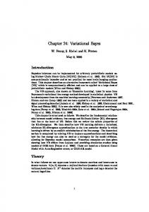
X = Xki ; k = 1, . . . , K; i = 1, . . . , P ; response surfaces of taxa. Superscript m and f stand for modern and fossil respectively. Notations without any superscript or subscript stand for both the types of variables, modern and ancient. Unlike that in Figure (1), the reported data on different taxa at various location in climate space are typically in counts. Due to huge variation in the tolerance limit of the taxa to different climate at different location, the count data on taxa are highly over-dispersed with an excess of zero counts in them. The zero-inflated behaviour of the count data can be understood with diagrams shown in Figure (2). The diagram represents the histograms of the count data on the taxa, Alnus and Corylus which shows that the most of the data points are zero.

1.3

Paper layout

In Section 2, we describe the model used for palaeoclimate reconstruction. Section 3 outlines the Bayesian inference approach, and implementation of the inference by variational Bayes is described in Section 4. Section 5 illustrates the approach with some examples.

2

Model description

For the demonstration of the Variational Bayes approximation to the palaeoclimate reconstruction problem, two types of the models are discussed in this paper; 1. one taxon and one climate model, 2. more than one taxon and one climate model.

3

8000

7000

7000

6000

6000 5000

Frequency

Frequency

5000 4000

3000

4000

3000 2000

2000

1000

0

1000

0

100

200

300

400

500

600

700

800

900

0

1000

0

100

200

300

400

500

600

Count data on taxon ’Corylus’

count data on taxon ’Alnus’

Figure 2: Histogram of the count data on the taxon (left) Alnus and (right) Corylus. The possible choices of the likelihoods of data on taxa and the prior distributions over the unknown parameters (ancient climate, response surface and hyper-parameters) are discussed for both the models.

2.1

The one taxon and one climate model

To explain the VB inference for the palaeoclimate reconstruction problem at a basic level, we first discuss the one taxon and one climate model. 1. Likelihood: It is assumed that the data on taxon are independent across the climate locations given the latent response surface. The ignorance of the dependence in data across the locations makes the inference problem simpler. It also favors the independent assumption of the VB method. Three standard distributions (likelihoods) are discussed for modelling data on taxa. (a) Gaussian Likelihood: For a simple understanding of the inference problem, data on taxa are first modelled with a Gaussian distribution. The VB approximation over the response surface is also Gaussian for a Gaussian prior distribution. L(y|X, θ) =

N !

N (yj ; X(Cj ), r 2 ).

(1)

j=1

As described earlier, data on taxon y are the function of the climate C through the latent responses X. At any climate location Cj , the mean of the Gaussian density of a data point yj is equal to the response surface, X(Cj ), a function of the climate at the same location; E(yj ) = X(Cj ). (2) The parameter r 2 is the unknown variance in the likelihood.

4

(b) Poisson Likelihood: A Gaussian density is not suitable for modelling count data on taxa. A Poisson distribution is one of the simplest choice among the discrete distributions to model count data. L(y|X, θ) =

N !

Poiss(yj ; exp(X(Cj ))).

(3)

j=1

In the Poisson likelihood L(y|X, θ), the mean is equal to exp(X(C)). Since the responses of the taxa to the climate can be both positive and negative, allowing the latent response surface raging from a negative value to a positive value in its space. The mean of the data point yj at Cth j climate location is an exponential function of the response surface X at the same location. E(yj ) = exp(X(Cj )). (4) (c) Zero-inflated Poisson Likelihood: The real data on taxa exhibit their zero-inflated behaviour (as shown in Figure 2). If zero-inflated data are modelled with a Poisson distribution, a non-zero-inflated distribution, the mean of the density would be underestimated and so the variance. The excess zeros in the data cannot even be ignored as they have potential information about the corresponding. Ridout et al. (1998) discuss a zero-inflated Poisson distribution for modelling counts with excess zeros; N ! L(y|X, θ) = ZIP (yj ; exp(X(Cj ))), (5) j=1

where ZIP (yj ; exp(X(Cj ))) =

"

1 − qj + qj exp(−eX(Cj ) ), if yj = 0; qj Poiss(yj ; exp(X(Cj ))), if yj > 0

where, (1 − qj ); j = 1 : N is the probability of observing essential zero counts. SalterTownshend (2009) uses a power law functional relationship to define the probability qj as # $γ λj qj = , (6) 1 + λj where, λj = exp(X(Cj )) is the rate parameter in the likelihood. The power index γ takes values from 0 to ∞ such that a big value of γ induces many zero counts in data. For a tractable VB approximation, we shall assume the probabilities of zeros inflation (1 − qj ); j = 1 : N , as known. The intractability issue of VB method with the unknown zeros inflation probabilities is explained in the Appendix section. 2. Prior Distributions: The two common unknowns to be inferred are the responses X and the ancient climate Cf . The climate space is assumed to be discrete and so climate values are taken on equally spaced discrete grid points. The discrete climate grid values are treated as the indexes for the response surfaces. (a) Prior distribution over ancient climate Cf : It is assumed that no particular information is available on the ancient climate to translate it into an informative prior

5

density. A non-informative prior is taken over the ancient climate assumed over discrete grid points; P (Cf ) ∝ 1. (7) (b) Prior distribution over response surface X: An intrinsic Gaussian Markov Random Field (IGMRF) by Rue and Held (2005) is assumed as a joint prior distribution over responses X across all the location in the climate space; P (X|Q) = IGMRF(Q).

(8)

IGMRF is an improper distribution with a low ranked precision matrix. The mean vector in the distribution is not specified. The markovian property of the GMRF allows the precision matrix Q to be sparse. Q = κ1 RP ×P ,

(9)

where, κ is an unknown smoothing parameter. The matrix R is a tri-diagonal matrix the first order random walk behaviour of the responses. In the case of a single climate variable, the IGMRF is specified as a Gaussian random walk indexed by climate: P ! P (X) ≈ NXi (Xi−1 , κ−1 ). (10) i=2

Generally, a multivariate Gaussian prior distribution is assumed as a prior distribution over a spatial variable. But often, the dense form of the covariance function in the distribution makes the computation slow. The advantage of a (intrinsic) GMRF over a multivariate Gaussian distribution is that it reduces the computation time, because the precision matrix in (intrinsic) GMRF is sparse. (c) Prior distribution over other unknown parameters: The prior distribution assumed over a smoothing parameter κ in an IGMRF prior, is a conjugate gamma prior with known hyper-parameters; κ ∼ Gamma(κ; a, b).

(11)

In the Gaussian likelihood, the variance parameter r 2 is assumed to be unknown. An inverse Gamma prior is considered over r 2 . r 2 ∼ Inv Gamma(r 2 ; α, β).

2.2

(12)

The more than one taxa and one climate model

As the palaeoclimate reconstruction is a multi-proxy problem, many taxa should be added to the model. We assume two taxa and one climate model. For the computational ease, the responses of each taxon are also considered as independent of each other. We add some unknown random effects to the latent responses in the model to induce dependence between taxa. For each data point (in modern and ancient ancient data set) on taxa, there is assumed a bivariate random effects (number 6

of dimensions equal to the number of taxa). Random effects also capture the over-dispersion in data. They are assumed to be independent of the climate in the model. U = {U1 , U2 }, Uk = ((Ukj )); k = 1, 2; j = 1 : N. 1. Likelihood: The Poisson likelihoods are considered to model count data on taxa. The taxa are assumed to be independent across climate location given the responses and are allowed to be independent of each other given the random effects. L(y1 , y2 |X1 , X2 , C, U1 , U2 ) =

2 ! N !

Poiss(ykj ; exp(Xk (Cj ) + Ukj )),

(13)

k=1 j=1

where, ykj denotes a data point on kth taxon at Cth j climate location, Xk is the corresponding unknown responses and Uj = (U1j , U2j ) is a common latent response at climate Cj that allows for dependence between taxa given climate, as described below. 2. Prior distributions: Independent IGMRF priors as described in the previous section are assumed over the responses X1 and X2 with precision matrix Q1 and Q2 and unknown smoothing parameters κ1 and κ2 . Conjugate Gamma priors are assumed over κ1 and κ2 with known hyper-parameters ak , bk ; k = 1, 2. The same non-informative prior distribution (as discussed for the one taxa and one climate) is assumed over the ancient climate Cf . A bivariate Gaussian distribution with zero mean and unknown covariance is assumed as an independent prior distribution over the random effects U for each of the data points on the taxa. #% & $ 0 −1 P (U|QU ) ≡ BVN U , QU . (14) 0 A Wishart distribution is considered as a prior distribution over the unknown precision Q−1 U ; QU ∼ Wishart(df, SS),

(15)

where df is the degree of freedom and SS is a symmetric positive definite matrix. The dimension of the matrix SS is same as the one of the precision matrix QU .

3

Bayesian Inference

The aim of the reconstruction problem is to first, model the response surface and second, to infer the ancient climate. The response surfaces are modelled through their indirect observation (the count data) on the pollen across all the climate location considered for the study of the ancient climate. Then, the unknown ancient climate is inferred through the knowledge obtained from the modelling of the response surface. In the Bayesian paradigm, the inference on an unknown variable is obtained through its posterior distribution. In the Bayesian approach to the palaeoclimate reconstruction problem, the joint posterior distribution of the response surfaces X the ancient climate Cf and other unknown parameters in the

7

model can computed by Bayes’ law, as L(ym |Cm , X, θ)L(yf |Cf , X, θ)P (X|Cm , Cf , θ)P (Cf )P (θ) . m m f f m f f f X,Cf L(y |C , X, θ)L(y |C , X, θ)P (X|C , C , θ)P (C )P (θ)dXdC (16) f All the unknown parameters (and hyper-parameters) other than X and C are denoted by θ. In the above expression for the joint posterior distribution P (X, Cf , θ|ym , Cm , yf ) given ym and Cm , the term L(ym |Cm , X, θ) is the likelihood of ym given Cm and X, whereas L(yf |Cf , X, θ) is the likelihood of yf . A prior density over ancient climate Cf is denoted by P (Cf ). The term P (X|Cm , Cf , θ) is a joint prior over responses X and P (θ) is a prior density over the parameters θ. The expression for the marginal posterior distribution of X after integrating out Cf and θ, is given as ( P (X, Cf , θ|ym , Cm , yf , ) = '

P (X|ym , Cm , yf ) =

P (X, Cf |ym , Cm , yf )P (θ)dCf dθ,

(17)

Cf ,θ

Similarly, the marginal posterior distribution of Cf is computed as ( f m m f P (C |y , C , y ) = P (X, Cf |ym , Cm , yf )P (θ)dXdθ.

(18)

X,θ

The marginal inference on Cf shown by above expression, is equivalent to the inverse inference on Cf discussed in Section 1. An inference on Cf requires the knowledge of X obtained from the marginal posterior distribution P (X|ym , Cm , yf ). Both the ancient climate Cf and the responses X depend on each other. The response surfaces X are high dimensional matrices (dimension equal to the total number of the climate locations in the study). For each taxon, there is a response surface across all the climate locations. The evaluation of the integrals over multi-dimensional responses surface makes the evaluation of the posterior distributions (joint and marginal) computationally intensive and intractable. The goal is to find a tractable approximation to Equation (16). In this paper the Bayes (VB) method is used for a tractable approximation of the posterior distributions. A brief introduction to the VB method is presented in the next section.

4 4.1

The Variational Bayes method A Brief Introduction

The Variational Bayes (VB) is a functional approximation for a posterior distribution that has an advantage of fast computation. In the VB method, we try to find a distribution qθ (θ) as an approximation to the intractable density P (θ|y) by minimizing a Kullback-Leibler divergence KL(qθ (θ) ' P (θ|y)): ( P (θ|y) KL(qθ (θ) ' P (θ|y)) = qθ (θ) log dθ. (19) qθ (θ) θ Kullback-Leibler (KL) divergence is a measure of discrepancy from one distribution to another. It ˇ ıdl and Quinn (2006) have discussed the KL divergence and is always a non-negative quantity. Sm´ its properties. Detailed discussion on KL divergence can be found in Kullback (1997). 8

In practice, it is not possible to find a minimum of KL(qθ (θ) ' P (θ|y)) with respect to qθ (θ), ie; qθ (θ) = arg min KL(qθ (θ) ' P (θ|y)), qθ (θ)

(20)

as the posterior distribution P (θ|y) is known only up to a proportionally constant. But, a solution to the minimum of KL(q(θ) ' P (θ|y)) may be found assuming the (posterior) independence between the components of the parameter θ in qθ (θ) i.e. qθ (θ) =

P !

qθi (θi )

(21)

i=1

where qθi (θi ) is a marginal approximation of posterior distribution over the ith component of θ, θi , also called the VB marginal (of θi ). With the assumption of posterior independence in θ, a minimum solution of KL(q(θ) ' P (θ|y)) with respect to qθi (θi ) as; q(θi ) ∝ exp[Eq(θ−i ) [log P (y, θ)]],

i = 1, · · · , d,

(22)

ˇ ıdl and Quinn (2006)). In the above expression, the VB approximation (see Theorem 3.3.1 of Sm´ ) over the components (other than θi ) of θ, qθ−i (θ−i ) = dj=1 qθj (θj ) is kept fixed. The term q(θi ) is j$=i

called the VB-marginal of θi .

The assumption of posterior independence allows the expectation in the R.H.S of Equation (22) being expressed as a tractable product of (d − 1) 1-dimensional expectation over the log-joint density log P (y, θ), with a condition that the log-joint density should factorize over the components of θ. For example, it is common to have factorized log-joint density over the components of the parameter for the exponential family of distributions. It can be seen from Equation (22) that the VB marginal qθi (θi ) is a function of the moments of θj , j (= i, with respect to qθ−i (θ−i ), which leads to the fact the VB-marginals interact with each other via their moments, or in other words, the moments of one VB-marginal is a function of the moments of other VB-marginals. The interdependence of the VB marginals present an obstacle in their evaluation. This requires an iterative (VB) algorithm for a local minima of KL(q(θ) ' P (θ|y)) ˇ ıdl and Quinn, 2006). (Sm´

4.2

Implementation of the method

In this section, the VB approximation to the reconstruction problem is explained. As described in Section 3, the aim of the problem is to find a tractable solution to the marginal posterior densities over latent response surface X and the unknown ancient climate Cf . The VB approximation for the joint posterior distribution P (X, Cf , θ) is given as P (X, Cf , θ) ≈ q(X, Cf , Uθ),

(23)

f

(24)

= qX (X)qCf (C )qU (U)qθ (θ).

The VB marginal qθ (θ) may be further decomposed into the VB marginals over the components of θ. 9

From Equation 22, the VB marginals qX (X), qCf (Cf ) and qθ (θ) are expressed as qX (X) ∝ exp[Eqθ (θ)q

Cf

(Cf )qU (U) [log P (y

m

, yf , Cf , X, U, θ|Cm )]],

qCf (Cf ) ∝ exp[Eqθ (θ)qX (X)qU (U) [log P (ym , yf , Cf , X, U, θ|Cm )]], qU (U) ∝ exp[Eqθ (θ)q

Cf

and, qθ (θ) ∝ exp[EqX (X)q

(Cf )qX (X) [log P (y

Cf

m

(Cf )qU (U) [log P (y

f

f

m

(25) (26)

, y , C , X, U, θ|C )]],

(27)

m

(28)

f

f

m

, y , C , X, U, θ|C )]],

where, the joint likelihood P (ym , yf , Cf , X, U, θ|Cm ) = L(ym |Cm , X, U, θ)L(yf |Cf , X, U, θ)P (X|Cm , Cf , θ)P (Cf )P (U|θ)P (θ). (29) The prior distributions over X and U are not conjugate to the likelihoods of Y. Hence, the VB marginal qX (X) and qU (U) may not be recognized as the standard distributions. A numerical integration method is used to compute the normalizing constant and the required moments of the intractable VB marginals. However, the method will be too time consuming for intractable multi-dimensional VB marginals. Rue and Held (2005) describes a quick way of finding Gaussian approximations to the intractable posterior distributions with GMRF or Gaussian priors. For a Gaussian approximation to an intractable posterior distribution, a quadratic approximation to the log-joint likelihood is considered. If the corresponding prior density is already a quadratic function (Gaussian or GMRF), we only need to find a quadratic approximation to the log-likelihood. We use the same idea of Rue and Held (2005) for Gaussian approximation of intractable VB marginals qX (X) and qU (U). The only difference is that we have VB-expectation of the log-joint likelihood with respect to the VB-marginals unknown parameters (presented in the Equation 28), which can further be decomposed in the log of prior term and the log of the likelihood terms depending on the VB moments of the other parameters.

4.3

VB solution to the one taxon and one climate model

VB solutions for the one taxon and one climate model with the likelihoods (discussed in Section 2.1) is presented. We present the VB marginals with their functional forms only. The functions are defined in detail in the Appendix section. 4.3.1

VB solution for the model with the Gaussian Likelihood:

The VB marginals over the responses surface X, the ancient climate Cf and the unknown variance r 2 are given as follows: 1. VB marginal over X obtained, is a Gaussian density with mean µX and variance σX and is expressed as qX (X) ≡ NX (µX , ΣX ), ΣX = µX =

10

Q#X−1 , Q#X BX ,

(30) (31) (32)

where BX is a function of likelihood terms involving y, data on pollen and the VB-moments of r 2 and Cf . The structure of the posterior (VB) precision matrix Q#X is given as Q#X = Eq (QX ) + diag(VX ),

(33)

= Eq (κ)R + diag(VX ),

(34)

where, QX is the prior precision. The term VX is the precision obtained from the likelihood and is a function of the data on pollen y and the VB-moments of r 2 and Cf . 2. The VB marginal over Cf , qCf (Cf ) is not a standard distribution. As the ancient climate Cf is univariate, a numerical approximation method can be applied to compute the normalizing constant of un-normalized qCf (Cf ). 3. The VB marginal over the variance parameter r 2 is an inverse Gamma density. qr2 (r 2 ) = Inverse Gamma(r 2 ; α# , β # ),

(35)

where, the hyper-parameters α# and β # are functions of the data y and the VB-moments of X and Cf . 4. The VB marginal κ, qκ (κ) is a Gamma density. qκ (κ) ≡ Gamma(κ; a# , b# ).

(36)

The hyper-parameters a# and b# in the VB marginal are functions of the VB moments of X and Cf . The smoothing parameter κ is independent of the likelihood of the data y. It appears only in the prior density of X. Therefore, the VB hyper-parameters do not involve any term related to the data y. 4.3.2

VB solution for the models with the Poisson and the zero-inflated Poisson Likelihood:

With IGMRF prior and a non-Gaussian likelihood (Poisson and zero-inflated Poisson Likelihoods), the VB marginal over the response surface X, qX (X) is not a tractable density. We apply a Gaussian approximation for a tractable approximation to qX (X). # qX (X) ≡ NX (µX , ΣX ),

ΣX = µX = Q#X

Q#X−1 , Q#X BX ,

(37) (38) (39)

= Eq (QX ) + diag(VX ),

(40)

= Eq (κ)R + diag(VX ),

(41)

BX = ((BXi )); i = 1 : P. th # Any (r, s)  element in the precision matrix QX has the following form;  2Eq (κ) + VXr , if r = s; Q#1 rs = −Eq (κ), r ∼ s;  0, otherwise.

11

(42)

% s are the functions of where, Eq (κ) is the VB mean of the smoothing parameters κ, VXr and BX i the first and the second derivatives of the VB expectation of log-likelihood at the posterior mode of X with respect to the other VB marginals. The VB-marginal over Cf , qCf (Cf ) is not a tractable density (as earlier in the Gaussian case). For the tractable inference to the problem, a numerical approximation is applied to compute the normalizing constants and so the moments of intractable uni-dimensional density qCf (Cf ). The VB marginal over κ is again a Gamma density with hyper-parameters as functions of X and Cf .

4.4

VB solution to the more than one taxon and one climate model:

In this section, we present the VB approximations to the marginal posterior distributions over Xk , κk , Uj and Cf for k = 1, 2. The VB marginals qXk (Xk ) over Xk ; k = 1, 2 with the GMRF priors and the Poisson likelihood, are not tractable. The structure of the Gaussian approximation to qXk (Xk ) is same as to the VB marginal of X described for the one taxa model. The VB marginals over the smoothing parameters κ1 and κ2 are Gamma densities. The hyperparameters of the density are functions of the VB-moments of the responses and of the ancient climate. The VB marginal over uni-dimensional ancient climate is intractable as for the one taxa model. The VB marginals over the bivariate random effects Uj ; j = 1 : N are also not tractable densities. The Gaussian approximation to the intractable VB marginals over Uj ; j = 1 : N is obtained as; # # qU (Uj ) = BVN (µ#Uj , QU ) j j

Q#Uj µ#Uj

(43)

= Eq (QU ) + diag(VUj )

(44)

= Q#U−1 BUj , j

(45)

where, the functions VUj = ((VUj k )); k = 1, 2 and BUj = ((BUj k )); k = 1, 2 depend on the first and second derivatives of the VB-expectation of the log-likelihood with respect to the other VB marginals. VB marginal over the prior precision QU of the random effects U is a conjugate Wishart distribution. qQU (QU ) = Wishart(df # , SS # ), (46) where, the hyper-parameters df # and SS # are the function of the VB-moments of the random effects Uj ; j = 1 : N .

5

Example

For the illustration of the VB approximation to the reconstruction problem, values are simulated from the likelihoods and the priors described in Section 2. A hundred regular spaced discrete values from 1 to 100 are assumed on climate location in the location space. Ten values are simulated on the climate from discrete uniform distribution, rages from 1 to 100. Vectors of 100 values on the response surfaces are generated from IGMRF prior densities. For the two taxa and one climate model, ten values on the bivariate random effects are derived from a bivariate Gaussian distribution. 12

Corresponding to each of the ten values on the climate, a data point on taxa is generated from the likelihoods described in Section 2. Nine of the ten values on the climate and the data on taxa are treated as the modern data and the tenth value on the data on taxa is used as ancient pollen data. The remaining one data point on the climate is assumed the true value on the ancient climate which is further used for the validation of the inference on the ancient climate. We present the results on the VB approximation to the two types of the models discussed in the paper. The results are presented separately for different choices of the likelihoods. 1. Result on one taxon and one climate model: The results on the modelling of the responses and the estimation of the ancient climate are shown in Figure (3) for different likelihoods. The figure shows the comparison between the VB means and the true values (simulated) of the response surface. The data on taxon are also displayed in the figure to represent the indirect observations on the true (latent) responses. In Figure 3 for the Poisson and the Zero-Inflated Poisson likelihoods, the log of the data points are shown as the indirect observations on the responses, as the responses are assumed to be the log-function of the count data in the likelihoods (rate parameters are the exponential function of the latent responses). The VB marginal over the ancient climate is also presented in the figure. The data points having the same at different climate locations result in the multi-modal VB approximation (VB marginal) over the ancient climate. 2. Result on the two taxa and one climate model: Figure (4) shows the VB approximations to the modelling of the responses for two taxa and that to the estimation of the ancient climate. The true responses and VB estimated responses are shown in the figure for the comparison of the result with the true value. The log of the data points minus estimated (VB) random effects as the indirect observations on the latent responses are also displayed in the figure (as the rate parameters assumed in the model is the exponential of the addition of the responses and the random effects at the observed locations). In Figures (3) and (4), the VB-means of the response surface pass through each of the modern data points, so are not a very smooth function of the data on taxa as they are desired. The VB marginal of the ancient climate is multi-modal due to the non-monotonic behaviour of the responses. The spiky modes of the VB marginal show the loss of some uncertainty in the estimation. The loss of accuracy in the estimation due to the posterior independence assumption of the VB method. It is clear from the figures that the VB-variance of the responses are small at the locations where data on taxa is available. For the Poisson and ZI-Poisson likelihoods the variance of the responses are much smaller than those for the Gaussian likelihood. Making Gaussian approximations for the tractable VB approximation forces us to lose some accuracy (the uncertainty). It also emphasizes on the fact that the VB method works well only for the exponential family of distributions and the conjugate priors. Though the Zero-Inflated Poisson model is capable of modelling the extra zero counts in data, the VB approximation over the ancient climate for the model is not very satisfactory (modes in the approximation are not close to the true value). The VB approximation requires some further approximations in the ZI-Poisson likelihood for the tractable solution which deteriorates the approximation on the inference on the ancient climate. It is clear from Figure (4) that the (VB) variance of the responses for the two taxa model are larger than those obtained for the one taxon model. So we gain in the uncertainty in the VB 13

0.25

15

10

0.2

5

VB marginal

response

0.15

0

0.1 −5

0.05 −10

−15

0

10

20

30

40

50 60 Climate/location

70

80

90

0

100

0

10

20

30

40

50 60 Ancinet climate

70

80

90

100

0

10

20

30

40

50 60 Ancient climate

70

80

90

100

0

10

20

30

40

50 60 Ancient climate

70

80

90

100

0.5

20

0.45 15

0.4 10

0.35

VB marginal

response

0.3 5

0

0.25

0.2

0.15

−5

0.1 −10

0.05

−15

0

10

20

30

40

50 60 Climate/location

70

80

90

0

100

20

0.5

15

0.45

0.4

10

0.35 5

VB marginal

response

0.3 0

−5

0.25

0.2 −10

0.15 −15

0.1

−20

−25

0.05

0

10

20

30

40

50 60 Climate/location

70

80

90

0

100

Figure 3: (Left) the black line denotes the true value of the response for the taxon, blue line is for the estimated response, red lines show the 95% HPD region, the blue asterisks represent the observations on taxon, the green asterisk stands for the data point on the taxon assumed as a single observation on the fossil pollen, (right) the VB marginal of the ancient climate given the observation on fossil pollen, the red asterisk shows the true (assumed) value of the ancient climate, the first block of the figures are for the Gaussian likelihood, second block, for the Poisson and the third is for the Zero-Inflated Poisson likelihood. marginal over the ancient by introducing the random effects in the two taxa and one climate model.

6

Discussion

VB provides a relatively fast functional approximation to a posterior distribution, through making assumptions of independence in the posterior. It presents a trade-off between ease of computation, via more independence assumptions, and accuracy of the approximation. Palaeoclimate reconstruction is a good example of its use in an inverse regression problem. 14

10

0.25

8 0.2

4

0.15 VB marginal

response surface of second taxon

6

2

0.1

0

−2 0.05

−4

−6

0

10

20

30

40

50 60 Climate/location

70

80

90

0

100

10

0

10

20

30

40

50 Climate

60

70

80

90

100

0

10

20

30

40

50 Climate

60

70

80

90

100

0.25

8 0.2

4 0.15 VB marginal

response surface of second taxon

6

2

0

0.1

−2

−4

0.05

−6

−8

0

10

20

30

40

50 60 Climate/location

70

80

90

0

100

Figure 4: (Left) the black line denotes the true value of the response for the first taxon, blue line is for the estimated response, red lines show the 95% HPD region, the blue asterisks represent the observations on taxon, the green asterisk stands for the data point on the taxon assumed as a single observation on the fossil pollen, (right) the VB marginal of the ancient climate given the observation on fossil pollen, the red asterisk shows the true (assumed) value of the ancient climate.

From the results for the model with Gaussian likelihood, it can be understood that the method performs well for the conjugate family of distributions. It provides tractable approximations to the intractable posterior distributions over unknown parameters for conjugate prior distributions. We can include many unknown parameters for estimation (assumed with the conjugate prior distributions) in the model. Unlike the MCMC method, the multi-modal behaviour of climate does not create any problem for a tractable VB solution. We learn (from Figures 3 and 4) that the VB method does have problems in convergence due to the multi-modal behaviour of climate. It performs quickly and provides a multi-modal VB-approximation to the multi-modal posterior distribution of the ancient climate. However, the resulting posterior distributions on climate appear to have smaller variance than desirable, in the sense that the true climate value is often not supported by the VB approximation. This is a commonly observed feature of VB approximations with some theoretical support (see Wang and Titterington (2004a), and Wang and Titterington (2004b)). VB approximations for intractable posterior distributions with non-conjugate distributions (likelihoods and priors) may not be recognized as standard distributions, which requires further approximations to the multi-dimensional VB approximations known up to proportionality constants. Gaussian approximations to intractable VB approximations with GMRF or Gaussian priors and non-conjugate likelihoods are presented in the paper. The VB approximation can be made more accurate by introducing the dependence between 15

taxa. But it may induce computational complexity in the inference problem. The assumption of random effects in the model, though increases the number of unknowns to estimate, but helps in gaining accuracy in the VB approximation without making the problem very complex. The zero-inflated Poisson distribution is the most appropriate of the three likelihoods for real data, but the VB implementation requires that the zero-inflation parameter is known. How to tractably incorporate inference for this parameter is clearly important. Since the responses of taxa to climate are latent and are modelled through the data on taxa, considering many more data points may smoothen the response surfaces. Making the inference problem not very complex and more accurate, the dependency between taxa can be allowed in nested structure, see (Salter-Townshend, 2009), keeping the intractability issue of the VB method in mind.

7

Bibliography

References Allen, R. M. J., W. A. Watts, and B. Huntley (2000). Weichselian palynostratigraphy, palaeovegetation and palaeoenvironment; the record from lago grande di monticchio, southern italy. Quaternary International 73–74, 91–110. Antonsson, K., S. J. Brooks, H. Sepp¨ a, R. J. Telford, H. John, and B. Birks (2006). Quantitative palaeotemperature records inferred from fossil pollen and chironomid assemblages from Lake Gilltj¨ arnen, northern central Sweden. 21 (8), 831–841. Bhattacharya, S. (2004). Importance Resampling MCMC: A Methodology for Cross–Validation in Inverse Problems and Its Applications in Model Assessment. Ph. D. thesis, Trinity College Dublin. Haslett, J., M. Whiley, S. Bhattacharya, M. Salter-Townshend, S. P. Wilson, J. R. M. Allen, B. Huntley, and F. J. G. Mitchell (2006, July). Bayesian palaeoclimate reconstruction. Journal of the Royal Statistical Society : Series A (Statistics in Society) 169 (3), 395–438. Huntley, B. (1991). How plants respond to climate change : , Migrate rates, individualism and consequences for plant communities. Annals of Botany 67, 15–22. Huntley, B., R. A. Spicer, W. G. Chaloner, and E. A. Jarzembowski (1993, August). The Use of Climate Response Surfaces to Reconstruct Palaeoclimate from Quaternary Pollen and Plant Macrofossil Data. Kullback, S. (1997, Oct). Information Theory and Statistics. Dover Publications Inc. Nakajima, S. and S. Watanabe (2006). Analytic Solution of Hierarchical Variational Bayes in Linear Inverse Problem. In ICANN (2), pp. 240–249. Ridout, M., G. B. Demetrio, and J. Hinde (1998). Models for count data with many zeros. In Proceedings of the XIXth International Biometric Conference, Invited Papers, pp. 179–192.

16

Rue, H. and L. Held (2005, February). Gaussian Markov random fields. Theory and applications (Monographs on Statistics and Applied Probability) (1 ed.). Chapman & Hall/CRC. Rue., H., S. Martino, and N. Chopin (2009). Approximate Bayesian Inference for Latent Gaussian Models by using Integrated Nested Laplace Approximations. Journal of the Royal Statistical Society Series B 71(2), 1–35. Salter-Townshend, M. (2009). Fast Approximate Inverse Bayesian Inference in non-parametric Multivariate Regression with application to palaeoclimate reconstruction. Ph. D. thesis, School of Computer Science and Statistics, Trinity College Dublin, Dublin 2, Ireland. ˇ ıdl, V. and A. Quinn (2006). The Variational Bayes Method in Signal Processing. Signals and Sm´ Communication Technology. Springer. Wang, B. and D. M. Titterington (2004a). Convergence and Asymptotic Normality of Variational Bayesian Approximations for Expon. In D. M. Chickering and J. Y. Halpern (Eds.), UAI, pp. 577–584. AUAI Press. Wang, B. and D. M. Titterington (2004b). Variational Bayes Estimation of Mixing Coefficients. In J. Winkler, M. Niranjan, and N. D. Lawrence (Eds.), Deterministic and Statistical Methods in Machine Learning, Volume 3635 of Lecture Notes in Computer Science, pp. 281–295. Springer.

8

Appendix

Gaussian Likelihood: For the VB marginal over X: for i = 1 : P ; VXi ni BXi

#

$ 1 = [ni + q(c = i)]Eq , r2 = No. of times i equals to C m ,   Nm 0  #1$  m f f =  yj + q(C = i)y  E 2 .   r f

j=1 Cjm =i

For the VB marginal over κ:

a# = a + 0.5(P − 1), % P P P −1 0 0 1 0 # f 2 f 2 b = b+ 2 q(C = i)Eq (Xi ) + q(C = i)Eq (Xi−1 ) + q(C f = i)Eq (X2i+1 ) 2 i=1 i=2 i=1 & P −1 P 0 0 −2 q(C f = i)Eq (Xi Xi−1 ) − 2 q(C f = i)Eq (Xi Xi+1 ) i=1

4

1 + 2 2

i=2

P −1 0

Eq (X2i ) + Eq (X21 ) + Eq (X2P ) − 2

i=2

P 0 i=2

17

5

Eq (Xi Xi−1 ) ,

For the VB marginal over r 2 : Nm , 2 & Nm% 1 0 m2 m 2 = β+ yj − 2yj Eq (X(Cj )) + Eq (X (Cj )) 2

α# = α + β#

j=1

% & P P 0 0 1 f2 f f f 2 + y − 2y q(C = i)Eq (Xi ) + q(C = i)Eq (Xi ) , 2 i=1

i=1

For VB marginal over Cf : for i = 2 : P − 1, # $# $ % 1 1 f f 2 q(C = i) ∝ exp − Eq y Xi + Xi 2 r2 " 6& 1 2 2 2 − Eq (κ) 2Xi + Xi−1 Xi+1 − 2Eq (Xi Xi−1 ) − 2Eq (Xi Xi+1 ) 2 Poisson Likelihood: For the VB marginal over X: for i = 1 : P ; VXi

BXi

M

= [ni + q(C f = i)]eXi , 



Nm 0   f f =  ym + q(C = i)y  − (1 − XM j i )VXi ,   j=1 Cjm =i

XM i

= Mode of the marginal posterior distribution over Xi .

The functional forms of the hyper-parameters of the VB marginal over κ are the same as those defined for Gaussian likelihood. For the VB marginal over Cf : for i = 2 : P − 1, % " 6 1 f 2 2 2 q(C = i) ∝ exp − Eq (κ) 2Xi + Xi−1 Xi+1 − 2Eq (Xi Xi−1 ) − 2Eq (Xi Xi+1 ) 2 " 6& Xi f + −Eq (e ) + y Eq (Xi ) Zero-Inflated Poisson Likelihood: For the VB marginal over X:

18

for i = 1 : P VXi =

%0 Nm

(1 −

Zjm ) +

j=1 Cjm =i M

−eXi

+e

XM i

e

& M q(C = i)(1 − Z ) eXi f

f

" 6−2 Nm % M M 0 −eXi XM m2 m2 m m −eXi i e e qj Zj 1 − qj + qj e

j=1 Cjm =i

" 6−1 & XM M +(1 − eXi )qjm Zjm 1 − qjm + qjm e−e i +e−e

XM i

% " 6−2 XM XM M M eXi q(C f = i) e−e i eXi q f 2 Z f 2 1 − q f + q f e−e i

XM i

+(1 − e

BXi

=

f

)q Z

f

−XM i VXi

"

f

M

f −eXi

1−q +q e

6−1 & ,

" 6 Nm % 0 M + (1 − Zjm ) eXi + yj j=1 Cjm =i

" 6−1 & XM M eXi qjm Zjm 1 − qjm + qjm e−e i % " 6 f f XM f i +q(C = i) (1 − Z ) e +y −e−e

f

XM i

+q Z e XM i

M

f −eXi

XM i

e

" 6−1 & M f f −eXi 1−q +q e ,

= Mode of the marginal posterior distribution over Xi . " 1, if ym j = 0; f m m Z and Zj ’s are the known auxiliary variables defined as Zj = 0, if ym j >0 " f 1, if y = 0; Zf = 0, if yf > 0 The functional forms of the hyper-parameters of the VB marginal over κ are the same as those defined for Gaussian likelihood. For the VB marginal over Cf : for i = 2 : P − 1, % " 6 1 f 2 2 2 q(C = i) ∝ exp − Eq (κ) 2Xi + Xi−1 Xi+1 − 2Eq (Xi Xi−1 ) − 2Eq (Xi Xi+1 ) 2 % " 6& " 6& 7 8 X +Z f Eq log 1 − q f + q f e−e i +(1 − Z f ) −Eq eXi + yf Eq (Xi ) 19

" 6 Xi f f −e Second order Taylor’s expansion of log 1 − q + q e around Xi = 0 is equal to −q f (1 − q f )e−e Considering further approximations to e−e

Xi

Xi

1 X + q f 2 e−2e i . 2

and e−2e

Xi

as

1 1 ≈ −eXi + e2Xi − e3Xi , 2 6 4 −2eXi Xi 2Xi e ≈ −2e + 2e − e3Xi 3 e−e

Xi

% " 6& % & 1 1 f f −eXi f Xi 2Xi 3Xi Eq log 1 − q + q e = q −Eq (e ) + Eq (e ) − Eq (e ) 2 6 % & 1 + q f 2 Eq (e2Xi ) − Eq (e3Xi ) 2 More than one taxa an done climate model: For the VB marginal over Xk k = 1 : 2: for i = 1 : P VXki

=

Nm % 9 m: 9 f:& M 0 Ukj f Eq e + q(C = i)Eq eUk eXki ; i = 1 : P,

j=1 Cjm =i

BXi





Nm 0   f f M =  ym + q(C = i)y kj k  − (1 − Xki )VXki ,   j=1 Cjm =i

XM i

= Mode of the marginal posterior distribution over Xi .

The functional forms of the hyper-parameters of the VB marginal over κ1 and κ2 are the same as those defined for Gaussian likelihood. The VB marginal over the random effects qU (U) =

m N !%

& qUf (Uf )

qUm (Um j ) j

j=1

For the VB marginal over Um j : for j = 1 : N m M

m

VUmkj

= eUkj Eq (eXk (Cj ) ),

m BU kj

M m = ym kj − (1 − Ukj )VUkj ,

UM kj

= Mode of the marginal posterior distribution over Um kj 20

and for the VB marginal over Uf : VUfk

Ufk

= e

M

6 P " 0 f Xki (Cf ) q(C = i)Eq (e ) , i=1

f BU k f M Uk

=

yfk

f − (1 − UM )VUfk , k

= Mode of the marginal posterior distribution over Ufk

For the VB marginal over QUj df # = df + N m + 1, %f f m SS # = SS −1 + Eq (U%m j Uj ) + Eq (Uj U ).

For the VB marginal over Cf : for i = 2 : P − 1 %0 " 6 2 % 1 2 2 2 − Eq (κk ) 2Xki + Xk(i−1) Xk(i+1) − 2Eq (Xki Xk(i−1) ) − 2Eq (Xki Xk(i+1) ) q(C = i) ∝ exp 2 " k=1 6&& f Xki + −Eq (e ) + yk Eq (Xki ) . f

21