Theoretical and numerical modelling of unvulcanized rubber ... branch model the ground-state viscoelasticity and rate-dependent hardening phenomenon.
Theoretical and numerical modelling of unvulcanized rubber H¨usn¨u Dal, Michael Kaliske & Christoph Zopf Institut f¨ur Statik und Dynamik der Tragwerke, Technische Universit¨at Dresden, Germany
ABSTRACT: The forming process of unvulcanized rubber is of great interest. However, classical hyperelastic models developed for cross-linked rubber do not apply to unvulcanized rubber due to the lack of crosslinks giving the material its elasticity. Experiments show that unvulcanized rubber exhibits strong viscoplastic flow without a distinct yield point accompanied with hardening. In this contribution, we propose a new constitutive model suited for unvulcanized rubber. The kinematic structure of the model is based on the micro-sphere model (see Miehe et al., JMPS 52:2617-2660, 2004). The computation of the stretch in the orientation direction follows the Cauchy-Born rule. The micro-sphere enables numerical integration over the sphere via finite summation of the orientation directions corresponding to the integration points over the sphere. This structure replaces the complex three-dimensional formulations, e.g. finite inelasticity models based on multiplicative split of the deformation gradient, by a simpler and more attractive one-dimensional rheological representation at the orientation directions. The rheology of the model consists of two parallel branches. The first branch consists of a spring connected to a Kelvin element where the latter spring models the kinematic hardening. The dashpot describes a time-independent endochronic flow rule based solely on the deformation history. The second branch consists of a spring connected to a Maxwell element in parallel to a dashpot. The two dashpots in the latter branch model the ground-state viscoelasticity and rate-dependent hardening phenomenon. Albeit its complexity, the proposed rheology and the numerical implementation show promising results suitable for large scale FE-based simulations.
1
INTRODUCTION
Rubber elasticity and inelasticity are active fields of research since decades. However, to the authors’ knowledge, no substantial effort exists on the modelling of unvulcanized rubber. Expansion of the simulation based design in all engineering processes increased the interest not only on the constitutive behaviour of the end products but also on the material behaviour of raw materials in parallel to the enhancements in the process simulation techniques. Within this context, we propose a one-dimensional rheology for unvulcanized rubber and its three-dimensional continuum extension within the context of the microsphere model, see Miehe et al. (2004). 1.1 Rheology The mechanical response of unvulcanized rubber is quite dissimilar to vulcanized rubber. Experiments demonstrate clearly that unvulcanized rubber is a highly deformable material which shows yield surface free equilibrium and non-equilibrium hysteresis with hardening at large strains. Unlike the classical viscoelastic behaviour of crosslinked rubber, it is ob-
served that the amount of hardening is also strongly rate dependent. The rheology of the model consists of two parallel branches with endochronic and viscoelastic dashpots accommodated in parallel to nonlinear springs responsible for the hardening. In the latter branch, the spring responsible for hardening is serially connected to a viscous dashpot in order to account for the rate dependent post-yield hardening phenomenon. In contrast to the crosslinked rubber, unvulcanized rubber does not show ground-state elasticity and material flows at very small strain rates without a distinct yield surface. Three different characteristics can be observed from experiments. Firstly, the material shows an equilibrium hysteresis up to moderate stretches which can be idealized by a serially connected elastic spring and a dashpot element converted from viscoelastic flow rule via the correspondence principle, see Haupt (2000). Further loading leads to post-yield hardening which is modeled via a spring connected in parallel to the friction element. Furthermore, at elevated loading rates, one observes strong rate effects around the thermodynamical equilibrium. The rheology representing the complexities inherent to the model is depicted in Fig. 2. Vulcanized rubber consists of a network connected via cross-links
which gives the material the memory for the undeformed state upon removal of the mechanical loading. Although unvulcanized rubber also posssesses a degree of elasticity due to the entanglements, the effect is small. The behaviour is nonlinear, showing significant equilibrium and non-equilibrium hysteresis. The cyclic loading of the material at low strain rates (cf. Fig. 5) shows that flow occurs even at very small deformation levels without a distinct yield surface. Further loading leads to kinematic hardening. Unvulcanized rubber shows significant rate dependency as depicted in the uniaxial tension tests, see Fig. 3a. The multistep relaxation test (cf. Fig. 4a) shows that the stresses do not fully relax reinforcing the hypothesis of existence of an equilibrium elastoplastic branch. Moreover, uniaxial tension experiments (Fig. 3a) clearly demonstrate a post-yield hardening regime which is strongly rate-dependent. Within this context, two discrete mechanisms are proposed for the description of the rheology of the material. For the equilibrium hysteresis observed at very small loading rates, a spring is connected serially to a Kelvin element, where an endochronic dashpot replaces the classical viscous dashpot via correspondence principle, see Haupt (2000). The spring in the Kelvin element models the rate-independent post-yield kinematic hardening regime. The latter branch consists of a non-linear spring connected serially to a system consisting of a Maxwell element in parallel to a viscous dashpot. The dashpot parallel to the Maxwell branch is responsible for the rate dependence of the initial loading whereas the dashpot in the Maxwell branch is responsible for the rate dependent kinematic hardening.
2
A MICROMECHANICAL MODEL FOR UNVULCANIZED RUBBER
2.1
Kinematic description
The key aspect of the micro-sphere based modelling is to link the deformation of a single point on the ¯. sphere to the macroscopic isochoric deformation F Let r denote√a Lagrangean orientation unit vector with |r|G := r ♭ · r = 1, where r ♭ := Gr is the covector of r obtained by mapping with the standard metric G = δAB . It can be described in terms of spherical coordinates r = cos ϕ sin ϑe1 + sin ϕ sin ϑe2 + cos ϑe3
in Cartesian frame {ei }i=1,2,3 , where ϕ ∈ [0, 2π] and ϑ ∈ [0, π], see Fig. 1. Mapping of the unit orientation vector r by the isochoric deformation of the contin¯ leads to the spatial orientation vector uum F t = Fr .
r3
ϑr ϕ r2
e2 r1
e1
is the co-vector of t obtained by a mapping with the current metric g = δAB . Before we introduce the averaging operator on the unit micro-sphere S, the infinitesimal R ϑ R ϕ area dA = sin ϑdϕdϑ and the area A(ϕ, ϑ) = 0 0 sin dϕdϑ are defined. The total area reads |S| = 4π. To this end, we define the averaging operator over the unit sphere S Z 1 (·) dA (4) h·i = |S| S which can be considered as the homogenization of the state variable (·) over the unit micro-sphere S. For the affine micro-sphere model, the macroscopic free energy function is linked to the microscopic free energies (5)
in terms of continuos integration on the sphere. The set of microscopic internal variables of are denoted by ¯ holds I . We propose, the affinity assumption λ = λ for the linkage between micro-stretches λ and macro¯ The affinity assumption corresponds to stretches λ. the Cauchy-Born rule in crystal elasticity, stating that for crystals undergoing small deformations, stretch in micro-orientation direction is equivalent to the macro¯ scopic stretch λ. 2.2
Figure 1. The unit micro-sphere and the orientation vector r = r1 e1 + r2 e2 + r3 e3 where r1 = cos ϕ sin ϑ, r2 = sin ϕ sin ϑ and r3 = cos ϑ in terms of spherical coordinates {ϕ, ϑ}, respectively.
(2)
The affine-stretch of a material line element in the orientation direction r reads √ ¯ := t♭ · t where t♭ := gt (3) λ
¯ Ψ(g; F , I) := nhψ(λ, I )i e3
(1)
Free energy and the dissipation function
A general internal variable formulation of finite inelasticity based on two scalar functions: the energy storage function and the dissipation function, will be constructed. The general set up of this generic type of models in the context of multiplicative split of
ψph ψp
The micro-dissipation due to the internal variable reads
γ˙ p
ep Dloc := βˆp ε˙p ≥ 0
ψvh γ˙ vh ψv
where we introduce the thermodynamical force driving the endochronic dashpot
γ˙ v
βˆp := −∂εp ψp − ∂εp ψph = βp − βph
Figure 2. Rheological representation of the proposed model
the deformation gradient dates back to the works of Biot (1965), Maugin (1990) among others. A similar framework is applied to rubber viscoelasticity by Miehe and G¨oktepe (2005) in the context of microsphere model. They used logarithmic stretches and internal variables in the orientation directions of the sphere with their work-conjugatetes for the description of the flow rule and/or the dissipation function. Such an ansatz circumvents the complexities inherent to the multiplicative split of the deformation gradient which entails additional assumptions concerning the inelastic rotation and inelastic spin. In what follows, we propose microscopic free energy functions and dissipation potentials for the constitutive description of the unvulcanized rubber material consistent with the rheological description depicted in Fig. 2. The microscopic free energy additively decomposes into elasto-plastic and visco-elastic parts ψ(λ, I ) = ψˆp (λ, I p ) + ψˆv (λ, I v ) .
(6)
The storage and dissipation functions describing each part will be considered as follows. Endochronic plasticity + kinematic hardening: The first branch of the rheology consists of two storage functions ψˆp (λ, I p ) = ψp (λep ) + ψph (λp ),
(7)
where the latter expression is responsible for the postyield kinematic hardening. A generic power-type expression is adopted for the free energy functions � µp ψp (λep ) := (λep )δp − 1 and (8) δp ψph (λp ) :=
µph (λp − 1)δph . δph
(9)
µp , δp , µph and δph are the material parameters. The stretch expression is split into elastic and plastic contributions λ = λep λp
and
ε := εep + εp ,
(10)
where ε = ln(λ), εep = ln(λep ) and εp = ln(λp ), respectively. Hence, the internal state of the material due to plastic deformation is described by I p := {εp } .
(12)
(11)
(13)
as work-conjugate to the logarithmic internal variable εp . βph = ∂εp ψph is the back stress. The model of inelasticity must be supplemented by additional constitutive equations which determine the evolution of the internal variables εp in time. A broad spectrum of inelastic solids is covered by the so-called standard dissipative media where the evolution ε˙p is governed by a smooth dissipation function φep which is related to the free energy function through Biot’s equation ∂εp ψp (εe ) + ∂ε˙ p φep (ε˙p , εp ) = 0
(14)
with εp (0) = 0. We propose a power-type generic expression for the dissipation function φep (ε˙p , εp ) :=
mp z˙ mp (ηp |ε˙p |) 1+mp ηp (1 + mp )
(15)
governed by the material parameters mp and ηp . Insertion of (15) into (14) leads to the evolution of the inelastic logarithmic strain after some manipulations ε˙p := γ˙ p (βˆp )βˆp
;
z˙ γ˙ p (βˆp ) := |βˆp |mp . ηp
(16)
A special choice of the evolution of the arclength z˙ := |ε| ˙ =
˙ |λ| λ
(17)
renders the formulation (16) rate-independent. Hence, the deformation of the plastic strain is controlled solely by the magnitude of the deformation history and plastic flow occurs without a distinct yield surface. Viscoelasticity + kinematic hardening: The second branch of the rheology also consists of two storage functions ψˆv (λ, I v ) = ψv (λve ) + ψvh (λvh ),
(18)
where the latter expression is responsible for the postyield kinematic hardening. A generic power-type expression is adopted for the free energy functions ψv (λve ) :=
� µv (λve )δv − 1 δv
ψvh (λvh ) :=
µvh (λvh − 1)δvh . δvh
and
(19) (20)
µv , δv , µvh and δvh are the material parameters. The stretch expression is split into elastic and viscous contributions λ = λve λv
and ε := εve + εv ,
(21)
where ε = ln(λ), εep = ln(λep ) and εp = ln(λp ), respectively. In order to model the rate-dependency of the hardening stress, a second dashpot is introduced. Accordingly, the viscous stretch and strain is decomposed as λv = λeh λvh
and
εv := εeh + εvh .
(22)
The internal state of the material due to viscous deformations is described by I v := {εv , εvh } .
(23)
The micro-dissipation due to the internal variables Table 1. Material parameters of the specified model Param. Description µp , δp µph , δph µv , δv µvh , δvh ηp , mp ηv , mv ηvh , mv
Elas. const., elasto-plastic branch Elas. const., back-stress in pl. branch Elas. const., visco-elastic branch Elas. const. back-stress in visc. branch Evol. par., plastic flow Evol. par., viscous flow Evol. par., hardening viscosity
Eqn. (8) (9) (19) (20) (15, 16) (27, 29) (28, 30)
1 |βvh |mv , (30) ηvh
respectively. In (16), (29) and (30), |(·)| := {[(·)/unit(·)]2 }1/2 is the norm operator with neutralization of the units. In addition, the material parameters of the specified model are listed in Table 1 along with their brief description and the equation numbers where they appear. 2.3
Stresses and Moduli
Endochronic plasticity + kinematic hardening: (i) Stresses: Having the free energy function and the dissipation function at hand, stress expression and the numerical tangent necessary for the finite element implementation will be derived. The Kirchhoff stresses τ¯ := ¯ ¯ , I) are computed via 2∂g Ψ(g; F τ¯ ep := hf p λ−1 t ⊗ ti
; f p :=
∂ ψˆp , ∂λ
(31)
with the help of the identity 2∂g λ = λ−1 t ⊗ t .
(32)
Applying the chain rule, the relation between the micro-stresses σp = ∂εe ψp and f p can be established f p = σp /λ .
reads ve Dloc := βˆv ε˙v + βvh ε˙vh ≥ 0 ,
(24)
where we introduce the thermodynamical forces driving the viscous dashpots βˆv := −∂εv ψv − ∂εv ψvh = βv − βvh
(25)
as work-conjugate to the logarithmic internal variable εv and βvh := −∂εvh ψvh
(26)
as work-conjugate to the logarithmic internal variable εvh , respectively. The identity ∂εv ψvh = −∂εvh ψvh is utilised in the previous equation. βvh = −∂εvh ψvh is the rate-dependent back stress. The power-type generic expressions for the dissipation functions read φve (ε˙v , εv ) :=
ε˙vh := γ˙ vh (βvh )βvh ; γ˙ vh (βvh ) :=
mv mv (ηv |ε˙v |) 1+mv , ηv (1 + mv )
(27)
mvh φ (ε˙vh , εvh ) := (28) (ηvh |ε˙vh |) ηvh (1 + mvh ) and are governed by the material parameters mv , mvh , ηv and ηvh , respectively. The dissipation potentials (27) and (28) lead to the evolution laws mvh 1+mvh
vh
ε˙v := γ˙ v (βˆv )βˆv
;
1 γ˙ v (βˆv ) := |βˆv |mv ηv
(31)2 and (33) into (8) leads to δ
λepp f = µp λ p
;
σp = µp λδepp .
(34)
Computation of σp at an orientation direction r entails the description of the current state of the history variable λp or εp . In order to compute εp for a given time-step tn+1 , we recall the flow rule expression (16) and recast it into a discrete residual form by backward Euler scheme r p = εp − εnp − γ˙ p (βˆp )βˆp ∆t = 0 .
(35)
The index n denotes the previous time-step tn , Table 2. Local Newton update of the internal variable εp 1. Set initial values DO 2. Residual equation 3.
Linearization
4.
Compute
5.
Solve
6.
Update
WHILE
and (29)
(33)
k = 0, ε0p = εn v ˆp )β ˆp ∆t = 0 r p = εp − εn ˙ p (β p −γ Lin r p
:= r p |εk + p
∂r p ∂εp
=0 |εk ∆εk+1 p p ∂r p Kp := ∂ε k p εp =εp
∆εk+1 = −K−1 p p rp
εk+1 ← εkp + ∆εk+1 p p k ←k+1 T OL ≤ |r p |
whereas the index n + 1 is dropped from εp and βˆp expression for the sake of convenience. The thermodynamical force driving the endochronic dashpot can be derived by incorporating (13)2 into (8) and (9)
p In order to derive the expression dε , we will make use dε ofpthe implicit function theorem. Recalling the identity dr = 0 and applying the chain rule, one finally ends dε up with
βˆp = σp − βph
∆t ηz˙p |βˆp |mp σp′ λep dεp = . dε Kp
; βph = µph (λp − 1)δph −1 λp . (36)
(35) is a nonlinear equation and cannot be solved analytically for εp . Linearization of the residual around εkp yields Lin r p := r p |εkp +
∂r p |εkp ∆εk+1 =0. p ∂εp
(37)
Setting ε0p = εnp , the incremental plastic strain in (37) can be obtained ∆εk+1 = −Kp−1 r p |εkp p
;
Kp =
∂r p |εk . ∂εp p
(38)
Viscoelasticity + kinematic hardening: (i) Stresses: The viscoelastic part of the Kirchhoff stresses can be derived similar to what has been proposed for the endochronic branch
εk+1 = εkp + ∆εk+1 . p p
(35) is to be solved repeating the steps (38) and (39) until a certain residual tolerance |rp |