Theoretical Results on Reinforcement Learning with ... - CiteSeerX

In Machine Learning: ECML’98. 10th European conference on Machine Learning, Chemnitz, Germany, April 1998. Proceedings, pp.382–393. Springer Verlag.

Theoretical Results on Reinforcement Learning with Temporally Abstract Options Doina Precup1 , Richard S. Sutton1 , and Satinder Singh2 1

Department of Computer Science University of Massachusetts Amherst, MA 01003-4610 http://www.cs.umass.edu/f˜dprecupj˜richg 2

Department of Computer Science University of Colorado Boulder, CO 80309-0430 http://www.cs.colorado.edu/˜baveja

Abstract. We present new theoretical results on planning within the framework of temporally abstract reinforcement learning (Precup & Sutton, 1997; Sutton, 1995). Temporal abstraction is a key step in any decision making system that involves planning and prediction. In temporally abstract reinforcement learning, the agent is allowed to choose among ”options”, whole courses of action that may be temporally extended, stochastic, and contingent on previous events. Examples of options include closed-loop policies such as picking up an object, as well as primitive actions such as joint torques. Knowledge about the consequences of options is represented by special structures called multi-time models. In this paper we focus on the theory of planning with multi-time models. We define new Bellman equations that are satisfied for sets of multi-time models. As a consequence, multi-time models can be used interchangeably with models of primitive actions in a variety of well-known planning methods including value iteration, policy improvement and policy iteration.

1 Introduction Model-based reinforcement learning offers a possible solution to the problem of integrating planning with real-time learning and decision-making [20]. However, conventional model-based reinforcement learning uses one-step models [11, 13, 18], that cannot represent common-sense, higher-level actions, such as picking an object or traveling to a specified location. Several researchers have proposed extending reinforcement learning to a higher level by treating entire closed-loop policies as actions [3–6, 9, 10, 12, 17]. In order to use such actions in planning, an agent needs the ability to create and handle models at a variety of different, interrelated levels of temporal abstraction. Sutton [19] introduced an approach to modeling at different time scales, based on prior work by Singh [17], Dayan [2] and by Sutton and Pinette [21]. This approach enables models of the environment at different temporal scales to be intermixed, producing temporally abstract models. In previous work [14], we generalized this approach from the prediction case, to the full control case. In this paper, we summarize the framework of temporally abstract reinforcement learning and present new theoretical results on planning with general options and temporally abstract models of options.

Options are similar to AI’s classical “macro operators” [7, 8, 16], in that they can take control for some period of time, determining the actions during that time, and in that one can choose among options much as one originally chose among primitive actions. However, classical macro operators are only a fixed sequence of actions, whereas options incorporate a general (possibly non-Markov) closed-loop policy and completion criterion. These generalizations are required when the environment is stochastic and uncertain with general goals, as in reinforcement learning and Markov decision processes (MDP). The predictive knowledge needed in order to plan using options can be represented through multi-time models [14]. Such models summarize several time scales and have the ability to predict events that can happen at various unknown moments. In this paper, we focus on the theoretical properties of multi-time models. We show formally that such models can be used interchangeably with models of primitive actions in a variety of well-known dynamic programming methods, while preserving the same guarantees of convergence to correct solutions. The benefit of using such temporally extended models is a significant improvement in the convergence rates of these algorithms.

2 Reinforcement Learning (MDP) Framework First we briefly summarize the mathematical framework of the reinforcement learning problem that we use in the paper. In this framework, a learning agent interacts with . At each time an environment at some discrete, lowest-level time scale = 0 1 2 step, the agent perceives the state of the environment, t , and on that basis chooses a primitive action, t . In response to each primitive action, t , the environment produces one step later a numerical reward, t+1 , and a next state, t+1 . The agent’s objective is to learn a policy , which is a mapping from states to probabilities of taking each action, that maximizes the expected discounted future reward from each state :

s

a

s

r

n

V  (s) = E r



r

r

t a s

; ; ;:::






s

o

s;  ; where 2 [0; 1) is a discount-rate parameter. The quantity V  (s) is called the value of state s under policy  , and V  is called the value function for policy  . The optimal value of a state is denoted  V (s) = max  V (s) 1

+

2

+

2

3

+

0

=

The environment is henceforth assumed to be a stationary, finite Markov decision process. We assume that the states are discrete and form a finite set, t 2 f1 2 g. The latter assumption is a temporary theoretical convenience; it is not a limitation of the ideas we present.

s

; ; : : :; n

3 Options In order to achieve faster planning, the agent should be able to predict what happens if it follows a certain course of action over a period of time. By a “course of action” we mean any way of behaving, i.e. any way of mapping representations of states to primitive actions. An option is a way of choosing actions that is initiated, takes control for some period of time, and then eventually ends. Options are defined by three elements:

– the set of states I in which the option applies – a decision rule which specifies what actions are executed by the option – a completion function which specifies the probability of completing the option on every time step.







is of a slightly more general form than the policies used in conventional reinforcement learning. The first generalization is based on the observation that primitive actions qualify as options: they are initiated in a state, take control for a while (one time step), and then end. Therefore, we allow to choose among options, rather than only among primitive actions. The conventional reinforcement learning setting also requires that a policy’s decision probabilities at time should be a function only of the current state t . This type of policy is called Markov. For the policy of a option, , we relax this assumption, and we allow the probabilities of selecting a sub-option to depend on all the states and actions from time 0 , when the option began executing, up through the current time, . We call policies of this more general class semi-Markov. The completion function can also be semi-Markov. This property enables us to describe various kinds of completion. Perhaps the simplest case is that of a option that completes after some fixed number of time steps (e.g. after 1 step, as in the case of primitive actions, or after steps, as in the case of a classical macro operator consisting of a sequence of actions). A slightly more general case is that in which the option completes during a certain time period, e.g. 10 to 15 time steps later. In this case, the completion function should specify the probability of completion for each of these time steps. The case which is probably the most useful in practice is the completion of a option with the occurrence of a critical state, often a state that we think of as a subgoal. For instance, the option pick-up-the-object could complete when the object is in the hand. This event occurs at a very specific moment in time, but this moment is indefinite, not known in advance. In this case, the completion function depends on the state history of the system, rather than explicitly on time. Lastly, if is always 0, the option does not complete. This is the case of usual policies used in reinforcement learning. Options are typically executed in a call-and-return fashion. Each option can be viewed as a “subroutine” which calls sub-options, according to its internal decision rule. When a sub-option 0 is selected, it takes control of the action choices until it completes. Upon completion, 0 transfers the control back to . also inherits the current time 0 and the current state t0 , and has to decide if it should terminate or pick a new suboption. Two options, and , can be composed to yield a new option, denoted , that first follows until it terminates and then follows until it terminates, also terminating the composed option .



t



s

t

t



n

n





o

o o

a

oo

s

a b ab

b

t

ab

4 Models of Options Planning in reinforcement learning refers to the use of models of the effects of actions to compute value functions, particularly . We use the term model for any structure that generates predictions based on the representation of the state of the system and on the course of action that the system is following.

V

In order to plan at the level of options, we need to have a knowledge representation form that predicts their consequences. The multi-time model of a option characterizes the states that result upon the option’s completion and the truncated return received along the way when the option is executed in various states [14]. Let p be an -vector and a scalar. The pair p is an accurate prediction for the execution of semi-Markov option in state if and only if

r

n

;r

o

s n r = E rt

+1

+

rt

+2

+






+ T rT st = s; o 1

n o p = E T sT st = s; o ;

and

T s s

o (1) (2)

o

where is the random variable denoting the time at which terminates when executed in t = , and sT denotes the unit basis -vector corresponding to T . p is called the state prediction vector and is called the reward prediction for state and option . We will use the notation “
”, as in x
y, to represents the inner or dot product between vectors. We will refer to the -th element of a vector x as ( ). The transpose of a vector x will be denoted by xT . The predictions corresponding to the states 62 I are always 0. If the option never terminates, the reward prediction is equal to the value function of the internal policy of the option, and the elements of p are all 0. The state prediction vectors for the same option in all the states are often grouped as the rows of an  state prediction matrix, P, and the reward predictions are often grouped as the components of an -component reward prediction vector, r. r P form the accurate model of the option. A key theoretical result refers to the way in which the model of a composed option can be obtained from the models of its components.

n

o

i

r

n n

s s xi

o

s

n

;

r;

Theorem 1 (Composition or Sequencing). Given an accurate prediction a pa for some option applied in state and an accurate model rb Pb for some option , the prediction: T = a + pa
rb and p = pa Pb (3)

a

s

;

g r

b

ab when it is executed in s. Proof. Let k be the random variable denoting the time at which a completes, and T be the random variable denoting the time at which ab completes. Then we have: r = Ert +


+ T rT j st = s; ab  k rk j st = s; a + E  k rk +


+ T rT j st = s; ab = E rt +


+ 1 X X Pfk = i j st = s; ag i Pfsk = s0 j st = s; k = ig = ra + is an accurate prediction for the composed option

+1

+1

i=1

1

1

+1

1

s0 T k 1 E rk+1 +


+ rT j s k = s 0 ; b 1 XX = ra + Pfk = i j st = s; ag iPfsk = s0 j st = s; k = igrb (s0) s0 i=1

X

ra + pa(s0 )rb (s0) s0 = r a + p a
rb

=

The equation for p follows similarly.

ut

A simple combination of models can also be used to predict the effect of probabilistic choice among options:

ri ; pi be a set of accurate predictions for the w > 0 be a set of numbers such that Pi wi = 1.

Theorem 2 (Averaging or Choice). Let options i executed in state , and let i Then the prediction defined by:

o

s

r= o

X

i

wi ri

p=

and

X

i

wi pi

(4)

s

is accurate for the option , which chooses in state among sub-options abilities i and then follows the chosen i until completion.

w

or

o

w E  rt

P

Proof. Based on the definition of , = i i P i i i The equation for p follows similarly.

wr

+1

+

oi with prob-




+ T rT j st = s; oi 1



=

ut

These results represent the basis for developing the theory of planning at the level of options. The options map the low-level MDP in a higher-level semi-Markov decision process (SMDP) [15], which we can solve using dynamic programming methods. We will now go into the details of this mapping.

5 Planning with Models of Options In this section, we extend the theoretical results of dynamic programming for the case in which the agent is allowed to use an arbitrary set of options, O. If O is exactly the set of primitive actions, then our results degenerate to the conventional case. We assume, for the sake of simplicity, that for any state , the set of options that apply in , denoted Os , is always non-empty. However, the theory that we present extends, with some additional complexity, to the case in which no options apply in certain states. Given a set of options O, we define a policy to be a mapping that, for any state specifies the probability of taking each option from Os . The value of is defined similarly to the conventional case, as the expected discounted reward if the policy is applied starting in :

s

s



s

s

n

V (s) = E rt

+1

+





rt

+2

+

o




st = s;  :

(5)

The optimal value function, given the set O, can be defined as

VO(s) =

s



sup

2O

V (s);

(6)

for all , where O is the set of policies that can be defined using the options from O. The value functions are sometimes represented as -vectors, V and VO , with each component representing the value of a different state.

n

The value function of any Markov policy equations: X

V  (s) =

 s; o r;

o2Os

 2 O satisfies the Bellman evaluation

(s; o)(ro + po
V);

for all

o

s

s 2 S;

(7)

where ( ) is the probability of choosing option in state when acting according to and o po is the accurate prediction for sub-option in state . We will show that, similarly to the conventional case, V is the unique solution to this system of equations. Similarly, the optimal value function given a set of options O satisfies the Bellman optimality equations:



 VO(s) = omax (r + po
VO); 2Os o

o

for all

s

s 2 S;

(8)

 is the unique solution of this set of equations, and there As in the conventional case, VO  2 O that is optimal, i.e., for which exists at least one deterministic Markov policy O    V O = VO. We will now present in detail the proofs leading to these theoretical results. The practical consequence is that all the usual update rules used in reinforcement learning  when the agent makes choices among options. We can be used to compute V and VO focus first on the Bellman policy evaluation equations.







Theorem 3 (Value Functions for Composed Policies). Let be a policy that, when starting in state , follows option and, when the option completes, follows policy 0 . Then ( ) = o + po
V0 (9)

s

o V s

r



:

Proof. According to the theorem statement, ately from the composition theorem.

 = o0 . The conclusion follows immediut

Theorem 4 (Bellman Policy Evaluation Equation). The value function of any Markov policy satisfies the Bellman policy evaluation equations (7).

 is Markov, we have: (s; o)V o (s)

Proof. Using the averaging rule and the fact that

V (s) = We can expand

X

o2Os

vo (s) using (9), to obtain the desired result (7).

ut

We now prove that the Bellman evaluation equations have a unique solution, and that this solution can be computed using the well-known algorithm of policy evaluation with successive approximations: start with arbitrary initial values 0 ( ) for all states and iterate for all : k+1 ( ) (s) + p(s)
Vk , where ( ) is the option suggested by in state .



s

sV

s

r

o

V s

s

s norm



Proof. For any option and any starting state , there exists a constant o such P that k po k1  o 1, where k
k1 denotes the 1 of a vector: k x k1 = i ( ). The value of o depends on and on the expected duration of when started in . For

 < 

l

o

xi s

o

T

r

any option , we show that the operator o (V) = o constant o . For arbitrary vectors V and V0 , we have:



To(V) To(V0 ) =

X

s0

+

po(s0)(V (s0) V 0(s0 )) 

po
V is a contraction with

X

po(s0 )k V V0 k1;

s0 where k
k1 denotes the l1 norm of a vector: k x k1 = maxi x(i). Therefore, To(V) To(V0 )  ok V V0 k1 The result follows from the contraction mapping

ut

theorem [1].

So far we have established that the value functions of Markov option policies have similar properties with the Markov policies that use only primitive actions. Now we establish similar results for the optimal value function that can be obtained when planning with a set of options. Theorem 5 (Bellman Optimality Equation). For any set of options  satisfies the Bellman optimality equations (8). value function VO



Proof. Let be an arbitrary policy which, at time step 0, in state among the available options with probabilities o .

V (s) =

W s

X

o2Os

w

wo(ro +

X

s

0

V s

Since

X

o2Os

0

=

s, chooses

po(s0)W (s0 ))

where  ( 0 ) is the expected discounted return from state using the definition of O( 0 ), we have:

V (s) 

s

O, the optimal

s0 on. Since po(s0)  0; 8s0,

 wo (ro + po
VO )  omax (r + po
VO) 2Os o

 is arbitrary, due to the definition of VO(s),  VO(s)  omax (r + po
VO): 2Os o o

r



 ). Let be the policy that On the other hand, let 0 = arg maxo2Os ( o + po
VO 0 chooses 0 at time step 0 and, after 0 ends, in state , switches to a policy s0 such that s0 ( 0 )  O( 0 ) . s0 exists because of the way in which O was defined. From (9), we have:

v s

o

V s

V (s) = ro0 +

X



po0 (s0)vs0 (s0 )  ro0 +

s0 Since VO(s)  v  (s), we have:



o

X

s0

s

V



po0 (s0)(VO(s0 ) )  ro0 + po0
VO 

  VO(s)  omax (r + po
VO) 2Os o

Since is arbitrary, it follows that

 t VO(s) = omax (r + po
VO) u 2Os o

The following step is to show that the solution of the Bellman optimality equations (8) is bounded and unique, and that it can be computed through a value iteration algorithm: start with arbitrary initial values 0 ( ) and iterate the update: k+1 ( ) maxo2Os o + po
Vk 8 .

r

V s

; s

V

T r

s

s

Proof. For any set of actions O let us consider the operator O which, in any state , performs the following transformation: Os (V) = maxo2Os ( o + po
V) Let V and V0 be two arbitrary vectors. Then we have:

T

0 0 TOs (V) = omax (r + po (V + V V0 )) = omax (T (V ) + po
(V V0 )) 2Os o 2Os o X  TOs (V0 ) + omax po(s0 )k V V0 k1 = TOs (V0 ) + Os k V V0 k1; 2Os

s0

Os = maxo2Os o. Similarly, TOs (V0 )  TOs (V) + Os k V V0 k1 Therefore, 8s, k TO (V) TO (V0 ) k1  O k V V0 k1 ; where O = maxs Os . Therefore TO is a contraction with constant O . The results where

follow from the contraction mapping theorem [1].

 is the unique bounded So far we have shown that the optimal value function VO solution of the Bellman optimality equations. Now we will show that this value function can be achieved by a deterministic Markov policy:

O defined as O (s) = arg omax r + po
VO 2Os o

Theorem 6 (Value Achievement). The policy

. achieves VO

s

Proof. For any arbitrary state , we have: 0

Since

 VO(s) V  s pO s
(VO VO )  Os k VO VO k1 :  O( ) =

( )

O < 1, VO(s) = V  s

 O( ).

ut

In order to find the optimal policy given a set of options, one can simply compute

VO and then use it to pick actions greedily. Another popular planning method for com-

puting optimal policies is policy iteration, which alternates steps of policy evaluation and policy improvement. We have already investigated policy evaluation, so we turn now to policy improvement:



Theorem 7 (Policy Improvement Theorem). For any Markov policy defined using options from a set O, let 0 be a new policy which, for some state , chooses greedily among the available options, and then follows



Then

V 0 (s)  V (s).

 0(s) = arg omax r + po
V; 2Os o

s

Proof. Let

o

0

 in state s. Then, from (7), r + po
V= V 0 (s):ut V (s) = ro0 + po0
V  omax 2Os o be the option chosen by

s

Given a set of options O such that Os is finite for all , the policy iteration algorithm,  in a finite which interleaves policy evaluation and policy improvement, converges to O number of steps. The final result relates the models of options to the optimal value function of the environment,  .

V

Theorem 8. If



ro ; po is an accurate prediction for some option b in state s, then ro + po
V  V (s)

We say that accurate models are non-overpromising, i.e. they never promise more that the agent can actually achieve.

o

Proof. Assume that the agent can use and all the primitive actions in the environment. Let =  , where  is the optimal policy of the environment. Then we have:

 o



V (s)  V  (s) = ro + po
V ut

6 Illustrations

g g

g g

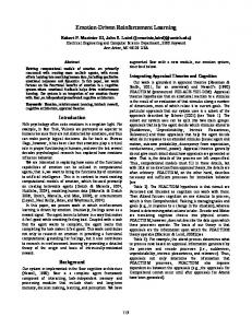
Average RMSE for all possible goal positions

The theoretical results presented so far show that accurate models of options can be used in all the planning algorithms typically employed for solving MDPs, with the same guarantees of convergence to correct plans as in the case of primitive actions. We will now illustrate the speedup that can be obtained when using these methods in two simple gridworld learning tasks. 0.6 0.5 0.4 0.3 0.2 Options

0.1

Primitives

0 0

2

4

6

8 10 12 14 Number of iterations

16

18

20

Fig. 1. Empty gridworld task. Options allow the error in the value function estimation to decrease more quickly

The first task is depicted on the left panel of figure 1. The cells of the grid correspond to the states of the environment. From any state the agent can perform one of four primitive actions, up, down, left or right. With probability 2/3, the actions cause the agent to move one cell in the corresponding direction (unless this would take the

agent into a wall, in which case it stays in the same state). With probability 1/3, the agent moves instead in one of the other three directions (unless this takes it into a wall, of course). There is no penalty for bumping into walls. In addition to these primitive actions, the agent can use four additional higher-level options, to travel to each of the marked locations. These locations have been chosen randomly inside the environment. Accurate models for all the options are also available. Both the options and their models have been learned during a prior random walk in the environment, using Q-learning [22] and the -model learning algorithm [19]. The agent is repeatedly given new goal positions and it needs to compute optimal paths to these positions as quickly as possible. In this experiment, we considered all possible goal positions. In each case, the value of the goal state is 1, there are no rewards along the way, and the discounting factor is = 0 9. We performed planning according to the standard value iteration method, where the starting values are 0 ( ) = 0 for all ) = 1. In the first experiment, the the states except the goal state, for which 0 ( agent was only allowed to use primitive actions, while in the second case, it used both the primitive actions and the higher-level options. The right panel in figure 1 shows the average root mean squared error in the estimate of the optimal value function over the whole environment. The average is computed over all possible positions of the goal state. The use of higher-level options introduces a significant speedup in convergence, even though the options have been chosen arbitrarily. Note that an iteration using all the options is slightly more expensive than an iteration using only primitive actions. This aspect can be improved by using more sophisticated methods of ordering the options before doing the update. However, such methods are beyond the scope of this paper.



: V goal

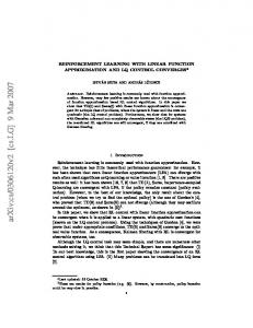
ROOM

HALLWAYS

V s

4 unreliable primitive actions up left

o1

right

Fail 33% of the time

down

G? o2

8 goal-directed options (to each room's 2 hallways)

Fig. 2. Example Task. The natural options are to move from room to room

In order to analyze in more detail the effect of options, let us consider a second environment. In this case, the gridworld has four “rooms”. The basic dynamics of the environment are the same as in the previous case. For each state in a room, two higherlevel options are available, which can take the agent to each of the hallways adjacent to the room. Each of these options has two outcome states: the target hallway, which corresponds to a successful outcome, and the state adjacent to the other hallway, which corresponds to failure (the agent has wandered out of the room). The completion function is therefore 0 for all the states except these outcome states, where it is 1. The policy underlying the option is the optimal policy for reaching the target hallway. The goal state can have an arbitrary position in any of the rooms, but for this illustration let us suppose that the goal is two steps down from the right hallway. The value of the goal state is 1, there are no rewards along the way, and the discounting factor







:

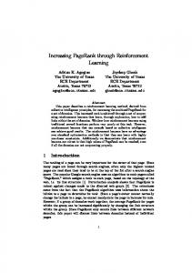
Iteration #1

Iteration #2

Iteration #3

Iteration #4

Iteration #5

Iteration #6

Fig. 3. Value iteration using primitive actions and higher-level options

is = 0 9. We performed planning again, according to the standard value iteration method, with the same setting as in the previous task. When using only primitive actions, the values are propagated one step on each iteration. After six iterations, for instance, only the states that are within six steps of the goal are attributed non-zero values. Figure 3 shows the value function after each iteration, using all available options. The area of the circle drawn in each state is proportional to the value attributed to the state. The first three iterations are identical to the case in which only primitive actions are used. However, once the values are propagated to the first hallway, all the states in the rooms adjacent to the hallway receive values as well. For the states in the room containing the goal, these values correspond to performing the option of getting into the right hallway, and then following the optimal primitive actions to get to the goal. At this point, a path to the goal is known from each state in the right half of the environment, even if the path is not optimal for all the states. After six iterations, an optimal policy is known for all the states in the environment.

7 Discussion Planning with multi-time models converges to correct solutions significantly faster than planning at the level of primitive actions. There are two intuitive reasons that justify this result. First, the temporal abstraction achieved by the models enables the agent to reason at a higher level. Second, the knowledge captured in the models only depends only on the MDP underlying the environment and on the option itself. The options and multi-time models can therefore be seen as an efficient means of transferring knowledge across different reinforcement learning tasks, as long as the dynamics of the environment are preserved. Theoretical results similar to the ones presented in this paper are also available for planning in optimal stopping tasks [1], as well as for a different regime of executing

options, which allows early termination. Further research will be devoted to integrating temporal and state abstraction, and to the issue of discovering useful options. Acknowledgments The authors thank Amy McGovern, Andy Fagg, Leo Zelevinsky, Manfred Huber and Ron Parr for helpful discussions and comments contributing to this paper. This research was supported in part by NSF grant ECS-9511805 to Andrew G. Barto and Richard S. Sutton, and by AFOSR grant AFOSR-F49620-96-1-0254 to Andrew G. Barto and Richard S. Sutton. Satinder Singh was supported by NSF grant IIS-9711753. Doina Precup also acknowledges the support of the Fulbright foundation.

References 1. Dimitri P. Bertsekas. Dynamic Programming: Deterministic and Stochastic Models. Prentice Hall, Englewood Cliffs, NJ, 1987. 2. Peter Dayan. Improving generalization for temporal difference learning: The successor representation. Neural Computation, 5:613–624, 1993. 3. Peter Dayan and Geoff E. Hinton. Feudal reinforcement learning. In Advances in Neural Information Processing Systems 5, pages 271–278. Morgan Kaufmann, 1993. 4. Thomas G. Dietterich. Hierarchical reinforcement learning with MAXQ value function decomposition. Technical report, Computer Science Department, Oregon State University, 1997. 5. Manfred Huber and Roderic A. Grupen. A feedback control structure for on-line learning tasks. Robotics and Autonomous Systems, 22(3-4):303–315, 1997. 6. Leslie P. Kaelbling. Hierarchical learning in stochastic domains: Preliminary results. In Proceedings of the Tenth International Conference on Machine Learning, pages 167–173. Morgan Kaufmann, 1993. 7. Richard E. Korf. Learning to Solve Problems by Searching for Macro-Operators. Pitman Publishing Ltd, 1985. 8. John E. Laird, Paul S. Rosenbloom, and Allan Newell. Chunking in SOAR: The anatomy of a general learning mechanism. Machine Learning, 1:11–46, 1986. 9. Sridhar Mahadevan and Jonathan Connell. Automatic programming of behavior-based robots using reinforcement learning. Artificial Intelligence, 55(2-3):311–365, 1992. 10. Amy McGovern, Richard S. Sutton, and Andrew H. Fagg. Roles of macro-actions in accelerating reinforcement learning. In Grace Hopper Celebration of Women in Computing, pages 13–17, 1997. 11. Andrew W. Moore and Chris G. Atkeson. Prioritized sweeping: Reinforcement learning with less data and less real time. Machine Learning, 13:103–130, 1993. 12. Ronald Parr and Stuart Russell. Reinforcement learning with hierarchies of machines. In Advances in Neural Information Processing Systems 10. MIT Press, 1998. 13. Jing Peng and John Williams. Efficient learning and planning within the Dyna framework. Adaptive Behavior, 4:323–334, 1993. 14. Doina Precup and Richard S. Sutton. Multi-time models for temporally abstract planning. In Advances in Neural Information Processing Systems 10 (Proceedings of NIPS’97), pages 1050–1056. MIT Press, 1998. 15. Martin L. Puterman. Markov Decision Processes: Discrete Stochastic Dynamic Programming. Wiley, 1994. 16. Earl D. Sacerdoti. A Structure for Plans and Behavior. Elsevier North-Holland, 1977. 17. Satinder P. Singh. Scaling reinforcement learning by learning variable temporal resolution models. In Proceedings of the Ninth International Conference on Machine Learning, pages 406–415. Morgan Kaufmann, 1992. 18. Richard S. Sutton. Integrating architectures for learning, planning, and reacting based on approximating dynamic programming. In Proceedings of the Seventh International Conference on Machine Learning ICML’90, pages 216–224. Morgan Kaufman, 1990. 19. Richard S. Sutton. TD models: Modeling the world as a mixture of time scales. In Proceedings of the Twelfth International Conference on Machine Learning, pages 531–539. Morgan Kaufmann, 1995. 20. Richard S. Sutton and Andrew G. Barto. Reinforcement Learning: An Introduction. MIT Press, 1998. 21. Richard S. Sutton and Brian Pinette. The learning of world models by connectionist networks. In Proceedings of the Seventh Annual Conference of the Cognitive Science Society, pages 54–64, 1985. 22. Christopher J. C. H. Watkins. Learning with Delayed Rewards. PhD thesis, Psychology Department, Cambridge University, Cambridge, UK, 1989.