Sep 17, 2013 - 1Nonlinear Physical Chemistry Unit, CP231, Faculté des Sciences, Université Libre de Bruxelles (ULB), 1050 Brussels, Belgium ... studied. Acid-base reactions are indeed exothermic reactions .... The mean distance between plumes is 3 mm. ... temperature T satisfy the following RDC evolution equations:.
PHYSICAL REVIEW E 88, 033009 (2013)
Thermal effects on the diffusive layer convection instability of an exothermic acid-base reaction front C. Almarcha,1,2 P. M. J. Trevelyan,1,3 P. Grosfils,4 and A. De Wit1 1
Nonlinear Physical Chemistry Unit, CP231, Facult´e des Sciences, Universit´e Libre de Bruxelles (ULB), 1050 Brussels, Belgium 2 Aix Marseille Universit´e, CNRS, Centrale Marseille, IRPHE UMR 7342, F-13384, Marseille, France 3 Division of Mathematics and Statistics, University of South Wales, CF37 1DL, United Kingdom 4 Center for Nonlinear Phenomena and Complex Systems, Universit´e Libre de Bruxelles (ULB), CP 231, 1050 Brussels, Belgium (Received 22 April 2013; published 17 September 2013) A buoyancy-driven hydrodynamic instability appearing when an aqueous acid solution of HCl overlies a denser alkaline aqueous solution of NaOH in a vertically oriented Hele-Shaw cell is studied both experimentally and theoretically. The peculiarity of this reactive convection pattern is its asymmetry with regard to the initial contact line between the two solutions as convective plumes develop in the acidic solution only. We investigate here by a linear stability analysis (LSA) of a reaction-diffusion-convection model of a simple A + B → C reaction the relative role of solutal versus thermal effects in the origin and location of this instability. We show that heat effects are much weaker than concentration-related ones such that the heat of reaction only plays a minor role on the dynamics. Computation of density profiles and of the stability analysis eigenfunctions confirm that the convective motions result from a diffusive layer convection mechanism whereby a locally unstable density stratification develops in the upper acidic layer because of the difference in the diffusion coefficients of the chemical species. The growth rate and wavelength of the pattern are determined experimentally as a function of the Brinkman parameter of the problem and compare favorably with the theoretical predictions of both LSA and nonlinear simulations. DOI: 10.1103/PhysRevE.88.033009
PACS number(s): 47.20.Bp, 47.70.Fw, 82.40.Ck
I. INTRODUCTION
Buoyancy-driven instabilities of miscible interfaces between reactive fluids impact a wide range of applications and physicochemical systems [1]. Among the various hydrodynamic instabilities that act on a stratification of a solution of A on top of another miscible solution of B in the gravity field, the most common one is the Rayleigh-Taylor (RT) instability [2,3] occurring when the density ρa of the upper solution of A is larger than the density ρb of the lower solution of B. If ρa < ρb , the system can nevertheless be destabilized either if B diffuses faster than A because of a so-called double-diffusion (DD) instability [3–6] or if diffusive-layer convection (DLC) is triggered when A diffuses faster than B [3,6–8]. In all cases, these buoyancy-driven instabilities lead in nonreactive miscible fluids to convective motions, which develop similarly above and below the initial contact line because of the symmetry of the underlying density gradient [2–8]. In reactive systems, it is of interest to understand how chemical reactions that influence the density profiles can impact these buoyancy-driven instabilities. Experimental studies of such hydrodynamic instabilities in reactive systems involving simple A + B → C type of reactions have characterized various patterns either in immiscible two-layer systems [9–17] or in miscible acid-base systems [18–26] for instance. In such miscible cases, the reaction can deeply affect the pattern as it has been shown to break the symmetry of RT, DD [26], and DLC [21,24] modes. From a theoretical point of view, the reaction-diffusion-convection (RDC) patterns are studied by coupling the equation for the flow velocity to evolution equations for the concentrations of the involved species via a state equation expressing the density as a function of the composition [21,26–30]. The comparison between experimental results and theoretical predictions is however confronted in such reactive 1539-3755/2013/88(3)/033009(11)
cases with several difficulties. First of all, the base state of the problem is time dependent as, upon contact, the miscible reactive solutions start to mix and reactions begin to operate, building complex density profiles in the system. To predict the wavelength and time of appearance of the related RDC pattern requires one to perform a linear stability analysis (LSA) of a time-dependent base state of a complex RDC system of equations. The question arises concerning the time at which to compare experimental and stability analysis data. Another issue relates to the way the patterns are visualized. Color indicators should ideally be avoided as they can be responsible for totally different patterns to what is seen in their absence [18,22,23] and because the patterns also depend on the type of color indicator used [19]. A solution is then to visualize gradients of the refractive index in the system but it remains to establish the link between these and density gradients or even further with concentrations gradients. Last but not least, the influence of thermal effects still needs to be quantitatively studied. Acid-base reactions are indeed exothermic reactions and, intuitively, it is reasonable to suppose that a local heating in the reaction zone, due to the exothermicity of the reaction, might lead to a local Rayleigh-B´enard type of mechanism whereby convection sets in above the reaction zone where the upper layer of fluid is heated from below. Double-diffusive effects due to differential diffusion of heat and mass are also susceptible to come into play [4,26,31]. Such thermally induced convective effects are well known to couple to reaction fronts [32–35]. Tanoue et al. [19] by placing a thermochromic liquid crystal sheet along the outside plane of the reactor associated to a local probe of the temperature in the cell by a thermocouple have shown that a temperature increase of the order of 0.5 K can be measured in the reaction zone for a simple HCl-NaOH system. More strikingly, hotter thermal plumes are found to rise following convective motions above
033009-1
©2013 American Physical Society
PHYSICAL REVIEW E 88, 033009 (2013)
ALMARCHA, TREVELYAN, GROSFILS, AND DE WIT
the reaction region. We have recently argued on the basis of simple quantitative estimation of related solutal and thermal Rayleigh numbers that thermal effects should be negligible in the dynamics of such acid-base fronts in Hele-Shaw cells [24]. The argument remains however heuristic as no linear stability analysis of the influence of thermal vs solutal effects has been performed in such systems. In this context, we revisit here both experimentally and theoretically reactive asymmetric DLC patterns observed when a simple exothermic neutralization reaction takes place inside a vertically orientated Hele-Shaw cell starting from an initially statically stable density stratification. Our objective is to investigate quantitatively the relative influence of solutal versus thermal effects in the hydrodynamic destabilization mechanism by performing a linear stability analysis of a RDC model of the problem taking specifically the influence of the exothermicity of the reaction on the density profile into account. The dynamics is described by reaction-diffusionconvection equations for the evolution of the concentration of the reactants A, B, product C, and of temperature T coupled to Darcy-Brinkman’s law for the evolution of the flow velocity. These predictions are compared to experimental data obtained using an interferometric method and particle image velocimetry (PIV) techniques to quantify the temporal evolution of the asymmetric convection and to measure the experimental growth rate and most unstable wave number of the early time perturbations. The goal is to compare experimental characteristic wavelengths and onset times of patterns with those predicted theoretically, respectively, both with and without heat effects. We demonstrate that, for the reaction and concentration ratios used in the experiments, the heat contribution to the instability characteristics is negligible. We also investigate the contribution of the various chemical species to the destabilization mechanism, showing that the instability indeed originates from differential diffusion phenomena involving the various chemical species diffusing at different rates rather than from a RayleighB´enard mechanism due to a localized heating by the reaction. Eventually, we also discuss the optimal time at which to compare experimental and theoretical growth rates and most unstable wave numbers showing good agreement between the two. We moreover discuss the influence of changes in the gap width of the cell and of initial concentrations on these values. The outline of the article is as follows. In Sec. II, the experimental procedure and observations are outlined. In Sec. III, the theoretical model is presented. In Sec. IV, the base state concentration and density profiles are numerically obtained. In Sec. V, a linear stability analysis is employed. In Sec. VI, nonlinear simulations are included. In Sec. VII, we summarize the results. II. EXPERIMENTAL RESULTS A. Experimental setup
The experimental setup consists of a vertically oriented Hele-Shaw cell made of two glass plates 3.1 cm wide and 5 cm high separated by a gap width h of either 0.5 or 1 mm. Using a specific device allowing a flat interface to be
y x
ACID A
g REACTION ZONE
BASE B
FIG. 1. Sketch of the system.
obtained between two miscible solutions [15], an aqueous HCl solution at concentration A0 is placed on top of an equimolar, miscible, and denser NaOH solution in the absence of any color indicator. A schematic diagram is illustrated in Fig. 1. Gravity points along the x direction while y denotes the transverse direction. xo is the initial position of the contact line. Once the reactants meet by diffusion the following exothermic reaction takes place: HClaq + NaOHaq → NaClaq + H2 O + heat B. Interferometric method
The visualization of the convective motions is performed via a PIV technique using chemically inert latex particles of diameter 5 µm. The visualization of the interface of the concentration patterns is obtained by digital interferometry based on a Mach-Zehnder type interferometer coupled with a CCD camera [36]. The light source is a 633 nm laser beam. The fringes, which are typically parallel in a homogeneous medium, are distorted in the presence of refractive index gradients. The phase shift "φ(x,y) = 2π h "n(x,y)/λ in the light beam (λ = 633 nm) induced by the local variation of the refractive index "n(x,y) in the Hele-Shaw cell is computed by a Fourier transform algorithm [37]. If necessary, the phase image is corrected by substracting a reference image in order to eliminate the possible misalignment of the Hele-Shaw cell window with the light beam. The method gives a precision of 10−5 on the value of the relative refractive index variation. An example of an interferometry figure is reported on Fig. 2 for molar solutions and a gap width h = 0.5 mm. C. Results
Soon after contact, a sinusoidal perturbation grows in the zone slightly above the initial position x0 . Later on, fingers develop, merge, and grow until they reach the upper limit of the reactor. Convective flows are observed to rise within fingers and sink between them (Fig. 3). Remarkably, the zone below x0 remains unperturbed by convection and features only a diffusive flux of solutes and a slow downward progression of the reaction front. The dynamics is thus fundamentally different from the one observed with similar acid-base systems in two-layer systems [11] or in the same system in the presence of a color indicator [18].
033009-2
PHYSICAL REVIEW E 88, 033009 (2013)
THERMAL EFFECTS ON THE DIFFUSIVE LAYER . . .
FIG. 2. Interferometric figure of asymmetric DLC obtained using a 1M HCl solution on top of an equimolar NaOH solution in a vertical Hele Shaw cell of gap width h = 0.5 mm. The height of the figure is 9.8 mm.
The origin of the instability can be understood in terms of a DLC mechanism as follows: The fast diffusing acid leaves the upper layer faster downwards than the base diffuses upwards. In the absence of any reaction, this difference in diffusivity would lead to a symmetric density profile with depletion of the fast diffusing species above and accumulation of it below the initial contact line respectively [3,6,21]. The resulting nonmonotonic density profile would then feature two distinct zones of convective motions that develop at symmetric distances from x0 in the nonreactive DLC [3,6]. The reactive system behaves differently because the acid cannot coexist with the base out of the reaction zone as it is swiftly consumed by the fast neutralization reaction. Hence, the depletion in acid in the upper solution is not followed by its accumulation in the lower solution. In the upper layer for a HCl solution initially on top of a NaOH solution, as the fast downward diffusion of H+ ions (D = 9.3 × 10⁻⁵ cm2 s−1 ) cannot be compensated by the slower upward diffusion of the Na+ ions (D = 1.3 × 10⁻⁵ cm2 s−1 ),
a local minimum in density appears above the initial contact line. The locally unfavorable stratification of a denser fluid on top of a less dense one induces convection in the upper layer through convective rolls. In the lower layer no convection rolls appear as no local maximum in the density appears below the initial contact line. The diffusion coefficient of the upward moving OH− ions (D = 5.3 × 10⁻⁵ cm2 s−1 ) is indeed larger than the diffusion coefficient of the incoming Cl− ions (D = 2.0 × 10⁻⁵ cm2 s−1 ). We can conclude that we have a nonsymmetric DLC instability: above the reaction zone, the diffusion of the species downward is faster than the diffusion of the species upwards while the reverse is operating under the reaction zone. In order to determine quantitatively the local evolution of density, the diffusion of ions must be considered in pairs. As the reaction is exothermic, a local heating of the solution in the reaction zone should reinforce this solutal mechanism by a Rayleigh-B´enard instability of the upper solution heated from below. Our objective is to quantify the relative importance of these two sources of instability by a theoretical analysis. III. THEORETICAL MODEL
In order to support the experimental findings and test the importance of thermal effects in the dynamics, let us now turn to a theoretical description of the problem. We assume that we have two miscible liquids, one containing an acid A, at initial concentration A0 , and the other containing a base B at initial concentration B0 . An exothermic neutralization reaction produces a salt C and heat via the mechanism
1.3425 1.342
1.3405
FIG. 3. (Color online) Superposition of the refractive index and velocity maps at time 70 s. Convection is observed only in the upper acidic solution. The mean distance between plumes is 3 mm. The height of the figure is 9.8 mm. The maximum velocity measured by PIV is 132 µm/s.
(2)
ρ = ρ0 [1 + αA A + αB B + αC C − αT (T − T0 )],
(3)
where ρ0 is the density of pure water at the temperature T0 and the molar expansion coefficients αi are defined as αi =
1.34 1.3395
2 1 1 = + , Dij Di Dj
where Di and Dj are the tabulated diffusion coefficients of the ions [38]. This allows one to reconstruct the density ρ in the system as a linear combination of the concentrations and temperature contributions as
1.3415 1.341
(1)
HCl and NaOH are a strong acid and base respectively, that totally dissociate into ions in water. However, to compute density profiles as a function of solutal expansion coefficients and concentrations we need to take as relevant variables the concentrations A, B, and C of HCl, NaOH, and NaCl ion pairs, respectively. These ion pairs are assumed to diffuse with a constant diffusion coefficient Dij computed as
1.3435 1.343
A + B → C + heat.
1 ∂ρ , ρ0 ∂Ci
where Ci is the concentration of the relevant chemical species. These coefficients are taken positive as the solutes are here increasing the solutal part of density. The thermal expansion coefficient is defined as 1 ∂ρ . αT = − ρ0 ∂T
033009-3
PHYSICAL REVIEW E 88, 033009 (2013)
ALMARCHA, TREVELYAN, GROSFILS, AND DE WIT
It is also considered as positive as we deal here with aqueous solutions at T > 4 ◦ C for which the density is a decreasing function of temperature. Consistently with the fact that the concentrations used are small, the temperature only varies by a few Kelvins so that the kinetic constant, the diffusion constants and the physical properties of water can be considered as independent of temperature. The three species concentrations A, B, and C along with the temperature T satisfy the following RDC evolution equations: At + u · ∇A = DA ∇ 2 A − qAB, Bt + u · ∇B = DB ∇ 2 B − qAB,
(4c)
∇ · u = 0,
(4e) µ 12µ 2 ∇p = − u + 2 ∇ u + ρ(A,B,C,T )g, (4f) K π where p is the pressure in the fluid. The permeability of the system is K = h2 /12. The dynamic viscosity and acceleration due to gravity are µ and g respectively. The 2D domain is considered infinite. The initial conditions for this problem are for for
x0
t , tc
u K , pˆ = (p − pa − ρ0 gx) uc lc µuc ρ0 cp 1 (A,B,C), θ = − (a,b,c) = (T − T0 ), A0 A0 "H xˆ =
x , lc
uˆ =
where hats denote a dimensionless quantity and g = |g|. The normalization speed, time, and length are αA A0 Kg DA uc = ,tc = 2 , and ν uc
ct + u · ∇c = δC ∇ 2 c + Da ab, θt + u · ∇θ = Le∇ 2 θ + Da ab,
DA lc = , uc
respectively, where ν = µ/ρ0 is the kinematic viscosity. The constant hydrostatic pressure and the ambient pressure pa have been used to define the dimensionless pressure. Additionally the dimensionless density is given by ρˆ = (ρ − ρ0 )/(αA A0 ). Substituting these nondimensional quantities into Eqs. (3)
(5a) (5b) (5c) (5d) (5e) (5f) (5g)
where i is the unit vector pointing downwards parallel to the x axis. The ratios of the expansion coefficients are RB =
αB , αA
RC =
αC αT "H , RT = − , αA ρ0 cp αA
(6)
As "H < 0 because the reaction is exothermic, RT > 0. The ratios of the diffusion coefficients are given by δB =
DB , DA
δC =
DC , DA
(7)
while Le = DT /DA is the Lewis number. Additionally, Da = qA0 tc
is the Damk¨ohler number, which is the ratio between the hydrodynamic normalization tc and the chemical tchem = 1/(qA0 ) time scales. Finally Br =
h2 π 2 lc2
is the Brinkman parameter quantifying the correction to Darcy’s law needed when the Hele-Shaw cell gap width is not sufficiently small with regard to the wavelength of the instability [39,40]. The initial conditions now become
where
where one recalls from Fig. 1 that x < 0 is the upper region and x > 0 is the lower region. We introduce the following nondimensionalization: tˆ =
ρ = a + RB b + RC c − RT θ, at + u · ∇a = ∇ 2 a − Da ab, bt + u · ∇b = δB ∇ 2 b − Da ab,
(4d)
where u is the velocity of the fluid, DA , DB , and DC are the molecular diffusion coefficients of A, B, and C, while cp is the constant pressure specific heat of water. DT is the thermal diffusivity, which is assumed not to depend on concentrations as the solutions are diluted. The kinetic constant of the neutralization reaction is q and "H is the enthalpy of the acid-base reaction. Although the density in the system changes due to both solutal and thermal contributions, relative changes are small enough so that the Boussinesq approximation can be made and the flow is treated as incompressible. The gap width averaged two-dimensional (2D) fluid flow inside the Hele-Shaw cell can be modeled to a good approximation by the Darcy-Brinkman equation [39], namely
T = T0 T = T0
∇ · u = 0, ∇p = −u + Br∇ 2 u + ρ(a,b,c,θ)i,
(4a) (4b)
Ct + u · ∇C = DC ∇ 2 C + qAB, "H Tt + u · ∇T = DT ∇ 2 T − qAB, ρ0 cp
A = A0 , B = 0, C = 0, A = 0, B = B0 , C = 0,
and (4) and dropping hats for convenience leads to the final dimensionless model
a = 1, b = 0, c = θ = 0 for x < 0, a = 0, b = γ , c = θ = 0 for x > 0, γ = B0 /A0
(8)
is the ratio between the initial concentrations of the base and the acid. For the specific case of the HCl-NaOH experiment, using the values of the parameters given in Table I fixes six of the parameters, i.e., RB = 2.22, RC = 2.17, RT = 0.16, δB = 0.61, δC = 0.50, and Le = 46. This study now only depends on the three remaining parameters Br, Da , and γ related to the geometry of the cell and to the initial concentrations. IV. BASE STATE OF THE SYSTEM
In order to analyze the stability of this system with regard to buoyancy-induced instabilities, we must first compute the base state of the pure reaction-diffusion problem. In the absence of flow, the one-dimensional reaction-diffusion base state profiles can be computed numerically by solving Eqs. (5d)–(5g) with u = 0. We let a(x,t), b(x,t), c(x,t), and θ (x,t) denote the base-state solutions. All of the base states approach self-similar
033009-4
PHYSICAL REVIEW E 88, 033009 (2013)
THERMAL EFFECTS ON THE DIFFUSIVE LAYER . . . TABLE I. Typical parameter values at 20 ◦ C for water [38]. Description
Parameter
Value
Kinetic constant Enthalpy of neutralization Specific heat Kinematic viscosity Gravity acceleration Density of water
q "H cp ν g ρ0
1.4 × 10¹¹ l/(mol s) −55.86 kJ/mol 4.182 kJ/(kg K) 9.2 × 10⁻⁷ m2 /s 9.8 m/s2 0.998 kg/l
HCl diffusion coefficient NaOH diffusion coefficient NaCl diffusion coefficient Thermal diffusivity HCl expansion coefficient NaOH expansion coefficient NaCl expansion coefficient Thermal expansion coefficient
DA DB DC DT αA αB αC αT
HCl optical index NaOH optical index NaCl optical index Thermal optical index
βA βB βC βT
3.34 × 10⁻⁹ m2 /s 2.13 × 10⁻⁹ m2 /s 1.61 × 10⁻⁹ m2 /s 1.4 × 10⁻⁷ m2 /s 1.8 × 10⁻² l mol−1 4.4 × 10⁻² l mol−1 4.1 × 10⁻² l mol−1 2.1 × 10⁻⁴ /K 0.0083 l mol−1 0.0098 l mol−1 0.0106 l mol−1 10−4 /K
A. Influence of the ratio of initial concentrations γ
profiles√ in the course of time with the similarity variable being η = x/ 4t. Using the obtained base-state concentrations, the dimensionless base-state density profiles can be reconstructed as ρ(x,t) = a + RB b + RC c − RT θ .
For γ = 1, as the acid diffuses faster than the base, the reaction front defined as the location of maximum C production invades the lower solution containing the base [41]. In parallel, a local minimum in the density profile is seen to develop around η = −0.784 in the upper layer. The temperature’s contribution to this density profile is found to be very weak because heat diffuses much faster than mass (Le ( 1) and because the value of RT is much smaller than the other solutal Rayleigh numbers. The contribution of thermal effects to the base-state density profile is therefore barely visible on Fig. 4. As thermal effects are barely affecting the density profile, they have a negligible effect on the dynamics as will be confirmed in Sec. V. The local minimum (illustrated in Fig. 4) is thus essentially due to the fact that the species A (acid) diffuses faster than the species C (salt) so this minimum in density corresponds to the zone, which is already depleted in acid while the salt has not had time to reach it yet. This unstable stratification of a locally denser zone on top of a less dense one in the upper layer is the origin of the convective instability observed above the contact line in the experiments.
(9)
In Fig. 4, each of the species contribution to the base state density profile are plotted as a function of η for γ = 1, i.e., equimolar initial concentrations. As a reminder, gravity points towards positive η. For η → ±∞, we are in the pure reactant solutions at ambient temperature (θ = 0). ρ = a = 1 in the pure acid reactant (b = c = 0) at η → −∞. In the alkaline zone where a = c = 0 while b = γ , the density ρ = RB γ . Any zone in the density profile featuring locally a minimum is susceptible to trigger buoyancy-driven flows as we have then locally a denser solution on top of a less dense one.
FIG. 4. Profiles of a, RB b, RC c, −RT θ and ρ for γ = 1. For our acid-base system here, RB = 2.22, RC = 2.17, RT = 0.16, δB = 0.61, δC = 0.50, and Le = 46.
We focus now on analyzing the effect of varying γ , i.e., the ratio of the initial concentrations, on the dynamics. By varying γ , using the large time asymptotic solutions [42], one finds that there are three different types of density profiles, which are illustrated in Fig. 5. If γ < 0.424, the density has a local minimum in the lower layer (η > 0), while if γ > 0.493 the density has a local minimum in the upper layer (η < 0). If 0.424 < γ < 0.493 then the density profile contains a local maximum sandwiched between two local minima. However, the most important factor that one must take into consideration is that when γ < 0.45 ≈ RB−1 the situation is initially stratifically unstable as the acid’s contribution to the density is then larger than the base’s contribution to the density. Thus to avoid a Rayleigh-Taylor instability one requires that γ > RB−1 . In order to determine when and where an instability occurs starting from an initially statically stable configuration
FIG. 5. Profiles of ρ for γ = 0 to 0.6 (solid line) in uniform increments of 0.15. Additionally, dotted lines are used to denote the special cases when γ = 0.424 and γ = 0.493.
033009-5
PHYSICAL REVIEW E 88, 033009 (2013)
ALMARCHA, TREVELYAN, GROSFILS, AND DE WIT
of a less dense solution on top of a denser one, we perform a linear stability analysis in the next section.
eigenvector F as F = MA + RB MB + RC MC − RT MT
(13)
σ v = J v,
(14)
to yield the eigenvalue problem
V. LINEAR STABILITY ANALYSIS A. Linear equations and numerical method
Using the base-state concentration and density profiles computed above, let us analyze the stability of the flow by LSA. As the flow is incompressible, for convenience, the stream-function formulation is employed. Using u = ψy and v = −ψx , we satisfy ∇ · u = 0. Taking the curl of Eq. (5b) yields 2
4
∇ ψ − Br∇ ψ = ay + RB by + RC cy − RT θy .
(10)
We introduce normal form perturbations to the base-state solutions in the form [ψ,a,b,c,θ] = [0,a,b,c,θ ] + /eσ t+iky [ik −1 F,A,B,C,T ], where / is a small parameter and make the quasi-steady-state approximation that the base-state solutions vary on a much slower time scale than the perturbations. Hence considering the base-state solutions frozen at a given time t0 , linearizing the resulting equations in / gives ρ = Fxx − k 2 F − Br(Fxxxx − 2k 2 Fxx + k 4 F) ,
(11a)
ρ = −k 2 (A + RB B + RC C − RT T ) , σ A = a x F + Axx − k 2 A − Da (aB + bA) ,
(11b) (11c)
σ B = bx F + δB (Bxx − k 2 B) − Da (aB + bA) , σ C = cx F + δC (Cxx − k 2 C) + Da (aB + bA) , σ T = θ x F + Le(Txx − k 2 T ) + Da (aB + bA) .
(11d) (11e) (11f)
These equations are solved numerically on a discrete set of points with the derivatives approximated using finite differences to allow the system to be expressed in matrix form as (L − BrL2 )F = k 2 (A + RB B + RC C − RT T ) , σA =
D (a) F x
σB =
D (b) F x
σC =
D (c) F x
(a)
(12a) (b)
+ LA − Da D B − Da D A ,
(12b)
(a)
(b)
+ δB LB − Da D B − Da D A ,
(12c) + δC LC + Da D B + Da D A , (a)
where v = (A,B,C,T )T and with
J = *
and
(12e)
where the fields F, A, B, C, and T are now represented in vector notation by F, A, B, C, and T . The diagonal matrix D (z) is constructed from the base-state solutions with its elements defined as Dij(z) = δij zi where z denotes a, b, c, and θ . Further, D (z) denotes the diagonal matrix obtained by differentiating x each element of D (z) with respect to x. The linear operator (∂x2 − k 2 ) is expressed in matrix format using finite differences as L. By writing M = k 2 (L − BrL2 )−1 one can express the
L + D (a) M − Da D (b) x D (b) M − Da D (b) x D (c) M + Da D (b) x
D (θ) M + Da D (b) x
RC D (a) M x
RC D (b) M x J ** = δC L + RC D (c) M x RC D (θ) M x
RB D (a) M − Da D (a) x
δB L + RB D (b) M − Da D (a) x (a) RB D (c) M + D D a x (θ) (a) RB D x M + D a D −RT D (a) M x −RT D (b) M x −RT D (c) M x
LeL − RT D (θ) M x
.
This method is similar to the approach used by Kalliadasis et al. in their LSA of buoyancy fingering of autocatalytic fronts [35]. The matrix M is numerically obtained using the subroutine DGESV from LAPACK and the eigenvalues and eigenvectors of J are obtained using DGEEVX from LAPACK. For a given fixed wave number k, the growth rate σ is then obtained numerically. As the base-state solution varies quickly at the start, this method is not valid for small values of t0 . In order to perform this numerical eigenvalue problem the infinite domain is truncated to a size w and the equations discretized using a nonuniform grid. The vertical spatial coordinate x is defined on a discrete set of N + 1 points as ) +1−2|j/N| w 16 * xj = j t0 + 1 N w
with the integer |j | ! N/2 so that √ |xj | ! w/2 and the mesh is finest around x0 = 0 with x1 ≈ 16 t0 /N. Grid independence was checked by increasing N until the variation in the maximum growth rate was below a given tolerance. Typically N = 200 was found to provide sufficiently accurate results.
(b)
(12d) (θ) (a) (b) σ T = D x F + LeLT + Da D B + Da D A .
" ! J = J * J **
B. Thermal effects
The base-state density profiles have a very weak dependence on the temperature. The linear stability analysis allows us to test whether these small thermal contributions have nevertheless an impact or not on the flow. In Fig. 6(a) the real part of the instantaneous growth rate σ is plotted as a function of the wave number k at various times for γ = Da = 1 and Br = 0 without thermal effects incorporated. At the onset of the instability the instantaneous growth rates are complex but in the course of time become real. Once the maximum growth rate is real, the rate of increase of the instantaneous growth rate increases in time. Still later a maximum is reached and then eventually σ decreases in time. This trend is also observed in the nonreactive DLC instability [3].
033009-6
PHYSICAL REVIEW E 88, 033009 (2013)
THERMAL EFFECTS ON THE DIFFUSIVE LAYER . . .
C. Quasi-steady-state approximation
(a)
We recall that the amplitude of the disturbances in the linear stability analysis are given by /eRe(σ )max t0 , so that no matter how small / is eventually the amplitude will become large and the linear stability analysis will break down. Further, the magnitude of the term Re(σ )max t0 is important in determining the order of the time at which the instability first becomes physically observable. As we are using the quasi-steady-state approximation, the growth rate depends on time. As the growth rates here are very small the linear stability analysis can remain valid until the time at which the term Re(σ )max t0 becomes O(1). This marks the end of the linear regime and the start of the nonlinear regime in which the dispersion curves of the LSA lose any meaning. (b)
D. Eigenfunctions
FIG. 6. (Color online) Real part of the instantaneous growth rates against the wave number k for γ = Da = 1 and Br = 0 in the isothermal case (a). The difference in the growth rate with the exothermic case is reported in (b), showing that the exothermic case for which RT = 0.16 is only slightly more unstable. The curves are illustrated at times t = 5000, 7000, 104 , 1.2 × 10⁴ , 1.5 × 10⁴ , 2 × 10⁴ , 3 × 10⁴ , 5 × 10⁴ , 105 , 3 × 10⁵ , and 106 from bottom to top and eventually right to left.
To determine the effect of the temperature, we compute the difference with the exothermic case with RT = 0.16 in Fig. 6(b). One can see that the exothermic growth rates are only slightly larger than the isothermal ones. The difference is indeed only of a few percents. This confirms that the effect of temperature is very weak in this problem. One finds that if RT is larger or Le is smaller then the temperature effects are enhanced, however, using the physically relevant parameters of Table I shows that the effect of the temperature can be ignored throughout the entire linear regime for the HCl-NaOH case. Thus the remainder of the linear stability analysis will focus on the isothermal case, setting RT = 0. In the presence of the temperature J is a 4N × 4N matrix, however, in its absence it reduces to a 3N × 3N matrix. As the cpu time of the eigenvalue problem scales with N 3 , the numerics takes less than half the time (27/64) in the absence of the temperature than in its presence, and so the removal of the temperature justified by its negligible impact is a useful approximation.
In Fig. 6(a), at t0 = 3 × 10⁴ the most unstable mode occurs with kmax = 0.0047 and σmax = 6.1 × 10⁻⁵ . We note that the term σmax t0 ≈ 1.8, which means that the system is nearing the end of the linear regime. We find that the most unstable mode is real. To determine where the instability occurs in space, the eigenfunctions associated with this most unstable mode are plotted at t0 = 3 × 10⁵ along with the base state solutions in Fig. 7. As the eigenfunction A is largest, all of the eigenfunctions were normalized with the maximum amplitude of A. In Fig. 7(a), each of the eigenfunctions A, B, and C are plotted along with the base-state concentrations a, b, and c. The eigenfunction B is around 102 times smaller than the other two eigenfunctions and its maximum value is just to the right of the reaction front, which is not observable in the figure. In Fig. 7(b), the eigenfunction F associated with the stream function, reconstructed using Eq. (13), is illustrated with the base-state density field. This shows that the instability is located in the upper layer (η < 0) where there is a local minimum in the base state of the density. More specifically, the instability is strongest approximately in the region where the density gradient is most negative, as expected since this is where the locally denser over less dense region is most unstable. The eigenfunctions have confirmed that the instability is only related to the eigenfunctions for species A and C while the eigenfunction for species B plays no part in the instability. These results confirm the important difference between reactive and nonreactive DLC instabilities in terms of both the shape of the eigenfunctions and the number of unstable modes at the end of the linear regime. In the reactive case studied here, we have one unstable mode with the eigenfunction associated with the stream function not changing sign. On the contrary, in the nonreactive DLC instability the eigenfunction associated with the most unstable mode takes a sign above the initial interface opposite to the sign below it [3]. Further in time in the nonreactive DLC instability, a second unstable mode appears and grows in time until both modes are equally dominant, but this second eigenfunction has the same sign above and below the initial interface. As the eigenfunctions are approximately equal in one region and equal and opposite in the other region, this allows the instabilities in each region to develop independently in the nonreactive case.
033009-7
PHYSICAL REVIEW E 88, 033009 (2013)
ALMARCHA, TREVELYAN, GROSFILS, AND DE WIT (a)
(a)
(b) (b)
FIG. 7. In (a) the eigenfunctions A, B, and C associated with the most unstable mode are plotted against η. In (b) the eigenfunction F associated with the most unstable mode is plotted against η. This is for the isothermal case with γ = Da = 1 and Br = 0 at t0 = 3 × 10⁵ . E. Effect of the Brinkman number Br
Returning to the reactive problem at hand, when it comes to comparing the experimental wavelength and growth rate of the instability with those in Fig. 6(a) the effect of the Brinkman number Br must be taken into consideration. The results in Fig. 6 were obtained using Br = 0 corresponding to the Darcy limit, which is valid when the gap width of the Hele-Shaw cell is sufficiently narrow. In dimensionless quantities, the linear stability analysis for Br = 0 overestimates the instability, i.e., predicts a shorter wavelength and a larger growth rate. However, by increasing the value of Br the dimensionless wavelength increases and the growth rate decreases. To demonstrate this the real part of the instantaneous growth rate σ is plotted in Fig. 8 as a function of the wave number k at various times for Br = 103 and Br = 104 when γ = Da = 1. Although we find that the qualitative results are the same as Br is increased, quantitatively there is a difference. By comparing Fig. 6(a) with Fig. 8(a), although we notice that increasing Br from 0 to 103 has a stabilizing effect, by the time t0 = 3 × 10⁴ there is only a small change with the wave
FIG. 8. (Color online) Real part of the instantaneous growth rates against the wave number k for γ = Da = 1, RT = 0, and (a) Br = 103 and (b) Br = 104 . In (a) the curves are illustrated at times t = 5000, 7000, 104 , 1.2 × 10⁴ , 1.5 × 10⁴ , 2 × 10⁴ , 3 × 10⁴ , 5 × 10⁴ , 105 , 3 × 10⁵ , and 106 and in (b) the curves are illustrated at times t = 104 , 1.2 × 10⁴ , 1.5 × 10⁴ , 2 × 10⁴ , 3 × 10⁴ , 5 × 10⁴ , 105 , 3 × 10⁵ , and 106 , from bottom to top and eventually right to left.
number around 7% smaller and the growth rate around 10% smaller. However, the differences increase as Br is increased further. In Fig. 8 the cases Br = 103 and Br = 104 are plotted over the same range of values to allow a better comparison. Although the two cases initially look very different, around t0 = 106 the two cases start to look the same, however, at this time the term σ t0 ≈ 30 and so the linear stability analysis is clearly not valid at this time. For Br < 103 , there is only a very small variation in the dispersion curves, meaning that the Darcy limit of Br = 0 is adequate to model this problem and the Brinkman correction term can be removed as was pointed out by Almarcha et al. [21]. However, when Br is increased above 103 , the growth rates become dampened so that the initiation of the instability is delayed and takes place over a longer time scale resulting in a larger wavelength of the instability. The asymptotic evolution of the wavelength and the growth rate with Br can be recovered considering Eq. (5b). For sufficiently high values (Br > 106 ) the term u can be neglected in front of the term Br∇ 2 u. Thus balancing Br∇ 2 u with ρ, of order one, we find that the product
033009-8
PHYSICAL REVIEW E 88, 033009 (2013)
THERMAL EFFECTS ON THE DIFFUSIVE LAYER . . .
TABLE II. The seven configurations tested experimentally, for several Hele-Shaw gap widths a and initial concentrations A0 . The value of the respective Brinkman parameter Br [40] and the normalization time and length used in model 5 are reported.
−5
2.5
x 10
2
configuration a (mm) A0 (M)
σ
1.5
1
0.5
0 0
0.5
1
1.5
k
2
2.5
3
3.5
−3
x 10
FIG. 9. Numerical dispersion relation computed by evaluating the variations between two successive time steps of the perturbations in concentration A for Br = 105 at times 2.8 × 105 , 3 × 10⁵ , 3.2 × 10⁵ , 3.4 × 10⁵ , and 3.6 × 10⁵
of time by length goes like Br. Then from Eq. (5d), balancing ∇ 2 a with at or with u.∇a, we see that the lengths scale like square root of time. So the growth rate scales like Br−2/3 and the wavelength scales like Br1/3 . These two asymptotes are verified experimentally and numerically in the following (Fig. 10). VI. NONLINEAR SIMULATIONS
The system of nonlinear equations (5) is numerically solved in the stream function formalism by the pseudospectral scheme proposed by Tan and Homsy [43], which has been adapted to take the chemical reaction into account. The program is based on the Fourier transform of the stream function ψ and of the concentrations of the reactants A and B, and of the product C. The system is integrated in two dimensions on a rectangular domain of dimensionless length L*x = Lx / lc and width L*y = Ly / lc . At the initial time, ψ = 0 and the concentrations of the chemical species are given by a step function. Noise is added on an intermediate line between the two levels of the step −4
growth rate
10
1 2 3 4 5 6 7
0.5 0.5 1 0.5 1 1 1
0.2 0.5 0.1 1 0.2 0.5 1
Br
tc (s) 3
1.39×10 8.72×10³ 2.23×10⁴ 3.49×10⁴ 8.93×10⁴ 5.58×10⁵ 2.23×10⁶
lc (mm) −3
5.96×10 9.54×10⁻⁴ 1.49×10⁻³ 2.38×10⁻⁴ 3.73×10⁻⁴ 5.96×10⁻⁵ 1.49×10⁻⁵
4.26×10⁻³ 1.71×10⁻³ 2.13×10⁻³ 8.53×10⁻⁴ 1.07×10⁻³ 4.26×10⁻⁴ 2.13×10⁻⁴
function in order to allow the emergence of the instability. The reaction rate is taken as unity (Da = 1). It still corresponds to a reaction time scale much smaller than the hydrodynamic time scales, as in the experiments. We computed the growth rate and wavelength of the perturbations of the early stages of the instability. The numerical domain width was chosen so that a minimum of 50 fingers were present at onset. The wavelength and largest growth rate were evaluated by computing the slope of the change between two successive computing times of the amplitude of each mode k in the Fourier transform of the concentrations and of the stream function. An example of related dispersion curves is reported on Fig. 9. We have checked once more that the difference between the growth rates, with and without thermal effects, remains within few percents. The growth rate at the end of the linear regime is reported on Fig. 10 and is always smaller than 6.6 × 10⁻⁵ , i.e., the upper limit value obtained for porous media (Br → 0). The most amplified wavelength at the onset of the nonlinear regime is also reported and we see a good agreement with numerics for all experiments performed for various values of the gap width and initial concentration A0 . The experimental wavelength and growth rate are calculated from Fourier transform of the PIV field in the early times of destabilization. Table II lists the various experimental conditions used as well as the corresponding value of the Brinkman parameter and normalization length
1.3435
−5
10
1.343 1.3425 −6
wavelength
10
2
10
10
5
10
4
10
3
10
4
Br
6
10
10
8
1.342 1.3415 1.341 1.3405 1.34
8
1.3395
FIG. 10. Experimental nondimensional growth rate and wavelength of the perturbations as a function of the Brinkman parameter Br, and comparison with numerical results shown as the dashed line.
FIG. 11. (Color online) Superposition of the numerical refractive index map and of the velocity map for same conditions as the experiment in Fig. 3.
10
2
10
4
Br
10
6
10
033009-9
PHYSICAL REVIEW E 88, 033009 (2013)
ALMARCHA, TREVELYAN, GROSFILS, AND DE WIT
and time allowing one to switch between dimensional and dimensionless variables. In the nonlinear regime, we also see a good agreement between experiments and numerics as reported on Fig. 11 where the refractive index computed using values from Table I is reported for the same conditions and at the same time as in Fig. 3. VII. CONCLUSION
In conclusion, we have studied experimentally buoyancydriven convection induced by a simple exothermic neutralization reaction between HCl and NaOH solutions in a vertical Hele-Shaw cell. The reaction drastically modifies the convective pattern with regard to the nonreactive equivalent, leading to an asymmetric situation where convection appears in the upper acidic solution only. A theoretical study based on a linear stability analysis and nonlinear simulations of a related reaction-diffusion-convection model has been performed to explore the relative weight of solutal versus thermal effects in the source of the instability. Contrary to what one might have expected, thermal effects are found to be weak in this problem. The heat of reaction is indeed found to virtually play
[1] A. De Wit, K. Eckert, and S. Kalliadasis, Chaos 22, 037101 (2012). [2] J. Fernandez, P. Kurowski, P. Petitjeans, and E. Meiburg, J. Fluid Mech. 451, 239 (2002). [3] P. M. J. Trevelyan, C. Almarcha, and A. De Wit, J. Fluid Mech. 670, 38 (2011). [4] J. S. Turner, Buoyancy effects in fluids (Cambridge University Press, Cambridge, 1979). [5] S. E. Pringle and R. J. Glass, J. Fluid Mech. 462, 161 (2002). [6] J. Carballido-Landeira, P. M. J. Trevelyan, C. Almarcha, and A. De Wit, Phys. Fluids 25, 024107 (2013). [7] R. W. Griffiths, J. Fluid Mech. 102, 221 (1981). [8] A. P. Stamp, G. O. Hughes, R. I. Nokes, and R. W. Griffiths, J. Fluid Mech. 372, 231 (1998). [9] D. Avnir and M. Kagan, Nature 307, 717 (1984). [10] O. Citri, M. L. Kagan, R. Kosloff, and D. Avnir, Langmuir 6, 3 (1990). [11] K. Eckert and A. Grahn, Phys. Rev. Lett. 82, 4436 (1999). [12] K. Eckert, M. Acker, and A. Grahn, Phys. Fluids 16, 385 (2004). [13] D. A. Bratsun, Y. Shi, K. Eckert, and A. De Wit, Europhys. Lett. 69, 746 (2005). [14] Y. Shi and K. Eckert, Chem. Eng. Sci. 61, 5523 (2006). [15] Y. Shi and K. Eckert, Chem. Eng. Sci. 63, 3560 (2008). [16] C. Wylock, S. Dehaeck, A. Rednikov, and P. Colinet, Microgravity Sci. Technol. 20, 171 (2008). [17] D. A. Bratsun and A. De Wit, Chem. Eng. Sci. 66, 5723 (2011). [18] A. Zalts, C. El Hasi, D. Rubio, A. Urena, and A. D’Onofrio, Phys. Rev. E 77, 015304 (2008). [19] K.-I. Tanoue, H. Ikemoto, M. Yoshitomi, and T. Nishimura, Therm. Sci. Eng. 17, 121 (2009). [20] K.-I. Tanoue, M. Yoshitomi, and T. Nishimura, J. Chem. Eng. Jpn. 42, 255 (2009).
a negligible role on the convection observed in this exothermic reaction problem. On the contrary, computation of the density profiles and the computation of eigenfunctions of the linear stability analysis confirm that the source of the instability is a double diffusive effect between HCl and NaCl. Indeed, the instability is found to be caused here by the salt product diffusing slower than the acid leading to a less dense region above the reaction front triggering a diffusive layer convection mechanism of instability. Quantitatively the theoretical model provides wavelengths and growth rates that follow the same trend and are of a similar order of magnitude to those in the experiments for all concentrations and Hele-Shaw cell gap widths scanned. A generalization of these results to classify the instability mechanisms possible for any kind of reacting solutions is currently in progress. ACKNOWLEDGMENTS
We thank Y. De Decker, A. D’Onofrio, K. Eckert, and A. Zalts for fruitful discussions. We thank F. Dubois for providing us access to his interferometric device. We acknowledge Prodex, FNRS and the ARC-CONVINCE programme for financial support.
[21] C. Almarcha, P. M. J. Trevelyan, P. Grosfils, and A. De Wit, Phys. Rev. Lett. 104, 044501 (2010). [22] C. Almarcha, P. M. J. Trevelyan, L. Riolfo, A. Zalts, C. El Hasi, A. D’Onofrio, and A. De Wit, J. Phys. Chem. Lett. 1, 752 (2010). [23] S. Kuster, L. A. Riolfo, A. Zalts, C. El Hasi, C. Almarcha, P. M. J. Trevelyan, A. De Wit, and A. D’Onofrio, Phys. Chem. Chem. Phys. 13, 17295 (2011). [24] C. Almarcha, Y. R’Honi, Y. De Decker, P. M. J. Trevelyan, K. Eckert, and A. De Wit, J. Phys. Chem. B 115, 9739 (2011). [25] K. Tsuji and S. C. M¨uller, J. Phys. Chem. Lett. 3, 977 (2012). [26] L. Lemaigre, M. A. Budroni, L. A. Riolfo, P. Grosfils, and A. De Wit, Phys. Fluids 25, 014103 (2013). [27] K. Eckert, L. Rongy, and A. De Wit, Phys. Chem. Chem. Phys. 14, 7337 (2012). [28] L. Rongy, P. M. J. Trevelyan, and A. De Wit, Phys. Rev. Lett. 101, 084503 (2008). [29] L. Rongy, P. M. J. Trevelyan, and A. De Wit, Chem. Eng. Sci. 65, 2382 (2010). [30] S. H. Hejazi and J. Azaiez, J. Fluid Mech. 695, 439 (2012). [31] J. D’Hernoncourt, A. Zebib, and A. De Wit, Chaos 17, 013109 (2007). [32] T. Bansagi Jr., D. Horvath, A. Toth, J. Yang, S. Kalliadasis, and A. De Wit, Phys. Rev. E 68, 055301 (2003). [33] V. V. Zhivonitko, I. V. Koptyug, and R. Z. Sagdeev, J. Phys. Chem. A 111, 4122 (2007). [34] J. Martin, N. Rakotomalala, L. Talon, and D. Salin, Phys. Rev. E 80, 055101(R) (2009). [35] S. Kalliadasis, J. Yang, and A. De Wit, Phys. Fluids 16, 1395 (2004). [36] P. Hariharan, Basics of Interferometry, 2nd ed. (Academic Press/Elsevier Inc., 2007).
033009-10
PHYSICAL REVIEW E 88, 033009 (2013)
THERMAL EFFECTS ON THE DIFFUSIVE LAYER . . . [37] M. Takeda, H. Ina, and S. Kobayashi, J. Opt. Soc. Am. 72, 156 (1982). [38] Handbook of Chemistry and Physics, 59th ed., edited by Robert C. Weast (CRC Press, Boca Raton, 1979). [39] J. Zeng, Y. C. Yortos, and D. Salin, Phys. Fluids 15, 3829 (2003).
[40] [41] [42] [43]
033009-11
H. C. Brinkman, Appl. Sci. Res. Sect. 1, 27 (1949). L. G´alfi and Z. R´acz, Phys. Rev A 38, 3151 (1988). M. Sinder and J. Pelleg, Phys. Rev. E 62, 3340 (2000). C. T. Tan and G. M. Homsy, Phys. Fluids 31, 1330 (1988).