762
IEEE TRANSACTIONS ON IMAGE PROCESSING, VOL. 8, NO. 6, JUNE 1999
Three-Dimensional Video Compression Using Subband/Wavelet Transform with Lower Buffering Requirements Hosam Khalil, Student Member, IEEE, Amir F. Atiya, Senior Member, IEEE, and Samir Shaheen, Member, IEEE
Abstract— Three-dimensional (3-D) video compression using wavelets decomposition along the temporal axis dictates that a number of video frames must be buffered to allow for the temporal decomposition. Buffering of frames allows for the temporal correlation to be made use of, and the larger the buffer the more effective the decomposition. One problem inherent in such a set up in interactive applications such as video conferencing, is that buffering translates into a corresponding time delay. In this paper, we show that 3-D coding of such image sequences can be achieved in the true sense of temporal direction decomposition but with much less buffering requirements. For a practical coder, this can be achieved by introducing an approximation to the way the transform coefficients are encoded. Applying wavelet decomposition using some types of filters may introduce edge errors, which become more prominent in short signal segments. We also present a solution to this problem for the Daubechies family of filters. Index Terms— Image sequence compression, 3-D wavelets, video conferencing.
I. INTRODUCTION
I
MAGE sequence coding has been an active research area for a long time. Video conferencing image sequence coding is becoming even more important now with the widespread use of networks and the affordability of video capturing equipments. In addition to spatial redundancies in the case of still images, video images possess temporal redundancies that have to be exploited in any efficient codec. Most video compression techniques utilize standard two-dimensional (2-D) compression methods, but with an added prediction step in the temporal dimension. The most widely used 2-D method utilizes the DCT, but also subband and wavelet transforms have provided very efficient techniques. Still image compression using wavelets is accomplished by applying the wavelet transform to decorrelate the image data, quantizing the resulting transform coefficients, and encoding the quantized values. This is usually carried out in a row-byManuscript received August 11, 1996; revised July 23, 1998. The associate editor coordinating the review of this manuscript and approving it for publication was Dr. Thrasyvoulos N. Pappas. H. Khalil is with the University of California, Santa Barbara, CA 93106 USA (e-mail:
[email protected]). A. Atiya is with the Department of Electrical Engineering, California Institute of Technology, Pasadena, CA 91125 USA (e-mail:
[email protected]). S. Shaheen is with the Department of Computer Engineering, Cairo University, Giza, Egypt. Publisher Item Identifier S 1057-7149(99)04064-6.
row then a column-by-column basis when using a separable one-dimensional (1-D) wavelet transform. A natural extension is to apply wavelet compression to a “3-D” image, with the temporal axis being the third dimension. Thus, in 3-D wavelet coding schemes, the frequency decomposition is carried out in addition along the temporal axis of a video signal. Slow movement in the video content will produce mostly low frequency components and the high frequency components will be almost negligible. This is the energy compacting property of wavelet decomposition, that would allow us to ignore some frequency components and still have a good representation of the signal. Recently, several 3-D wavelet/subband coding schemes have appeared. Wavelet/subband coding lends itself to scalable techniques and one such technique was presented in [1]. The multirate scheme uses global camera-pan compensation and supports multiple-resolution decoder displays. In [2], an adaptive scheme in which the decomposition along the temporal direction utilizes more or less frames depending on video activity. Typically, less frames would be used when activity is high (correlation is low). In [3], a scheme is presented that uses wavelet packets. Yet another scheme utilizing 3-D subband coding is described in [4] demonstrating 3-D zero-tree coding. Other schemes such as [5]–[9] are basically hybrid-like schemes with correlation only between two adjacent frames utilized. The obvious advantage of utilizing a temporal decomposition is that representation of temporal changes can be very efficient in the transform domain when movement is slow. The forward transform is implemented using analysis filters, and, generally, better analysis is achieved when filters are longer so that correlation among more frames can be discovered. One problem inherent in such a scheme is that if it is required to analyze video over long sequences, one must first buffer a large number of frames. Such a requirement is not a problem when considering general video such as in [1]–[4]. But in interactive applications such as video phone, buffering of frames results in a corresponding time delay. If there is a maximum allowable delay in such applications, that would put an upper limit on the number of frames that can be used for our decomposition resulting in lower compression efficiency. Previously, this problem was solved by using only Haar wavelets (a filter with a length of two taps) in the temporal direction. One even simpler solution was to treat only a maximum of two consecutive frames (i.e., a maximum
1057–7149/99$10.00 1999 IEEE
KHALIL et al.: 3-D VIDEO COMPRESSION
763
of one decomposition level in the temporal direction), and thus is very similar in nature to normal hybrid coding techniques. Examples of such codecs can be found in [5]–[9]. In this paper, we propose a solution to this problem by allowing correlation over a larger number of frames to be utilized while operating below the maximum allowable delay. Such a scheme is made possible by applying the temporal decomposition to a window of frames consisting of some old frames and a number of new frames as dictated by the maximum allowable delay. Selective transmission of coefficients concerning only the new frames is then performed. The next section explains the use of wavelets and Sections III and IV present the details of the video coding algorithm. Results and conclusions will be presented in Sections V and VI, respectively. II. THE SUBBAND/WAVELET TRANSFORM Still images are considered as 2-D signals. Applying the subband/wavelet transform to such signals is most commonly done by using the 1-D transform version and applying it to the still image in both row-order and column-order. This is because implementation of the single dimension transform is more efficient than an equivalent 2-D transform, and was shown [10] to be an effective solution. Video images can be considered as a 3-D signal, the three dimensions being the horizontal, the vertical, and the temporal dimension. In this section, we will summarize the implementation of the 1-D wavelet transform which is also representative of the subband transform in this context. The wavelet transform, as a data decorrelating tool, has won acceptance because of its multiresolution analysis capabilities in which the signal being transformed is analyzed at many different scales to give a transformation whose coefficients can efficiently describe fine details as well as global details in a systematic way. This, in addition to the locality of the wavelet basis functions as opposed to the Fourier transform, for example, which uses infinite width basis functions. Wavelets also unify the many other techniques that are of local type, such as the Gabor transform and the short time Fourier transform. The wavelet/subband transform is implemented using a pair of filters: a highpass filter and a lowpass filter , which split a signal’s bandwidth in two halves. The frequency responses and are mirror images. To reconstruct the original of signal an inverse transform is implemented, using the inverse , which are also mirror images. transform filters The 1-D forward wavelet transform of a discrete-time signal , is performed by convoluting that signal with and downsampling by two. Specifically, the both , and analysis cycle is (1)
(2) represent the lowpass downsampled result, the where highpass downsampled result, and and , respectively, are
the coefficients of the discrete-time filters and with filter taps. The synthesis cycle (backward transform) is performed as follows: (3) where the ’s represent the synthesized values after an analwhenever ysis/synthesis cycle and is odd. Also, and , respectively, are the coefficients of the discrete-time filters , and . Perfect reconstruction . By downsampling, as requires that implied by (1) and (2), we are in effect producing a critically subsampled set. This is possible because the analysis filters each result in a half-bandwidth output. A common problem arises with respect to edges, and is well known as the “edge-problem” in wavelet/subband coding. Basically, the problem does not arise in infinite-length signals, but practically, we only transform a limited-length signal such as a row of pixel values in an image. When applying (1) and (2), we immediately see that we would need to extend the signal beyond the edges, to provide all required coefficients in those equations. This problem occurs again in (3). We can assume some suitable values for the extension, but if exact reconstruction will be required, then the values of the referenced elements that are outside our initial set that are used in the analysis cycle need to be retained so that they can be used again in the synthesis cycle. The disadvantage of this is that the number of elements (samples) that have to be retained will be larger than the original set and thus if recursive application of the transform will be applied, the data set size will continue to rise and thus not constitute a critically sampled data set. On the other hand, the requirement that the number of elements necessary for representation to remain constant is stated as follows: The highpass and lowpass filtering of a should result in outputs and 1-D signal of length with a total number of samples that is also . Some methods [11] have been used to solve this problem, and generally all of them extend the 1-D signal to counter the effect of finite signal length. One extension method that involves wrapping the image around the edges to form a periodical signal provides perfect reconstruction but when subjected to high quantization still produces degradation at the edges. Another method that makes a mirror extension at the edges may produce less degradation but may not give perfect reconstruction for some filters. In this work, we use two types of wavelets. The symmetric -tap filters of [12] for the spatial directions, and the 6tap Daubechies filter [13], [14] for the temporal direction. The symmetric extension at the edges are suitable for the former filter, but inappropriate for the latter. Because we are compelled to use the combination of these filters, as will be explained in Section III, we use a new extension technique that provides perfect reconstruction for Daubechies filters (that we use for the temporal dimension) even at the edges. This new technique is explained in the appendix so as not to distract from the main topic of this work.
764
IEEE TRANSACTIONS ON IMAGE PROCESSING, VOL. 8, NO. 6, JUNE 1999
III. THREE-DIMENSIONAL WAVELET CODING In this section, we propose a coding system utilizing a 3-D wavelet transform that will be able to handle interactive applications. We use separable wavelets for our decomposition, whereby 1-D wavelets are used in each of the three dimensions. We essentially perform the three steps of horizontal decomposition, then vertical decomposition, then temporal decomposition. When we apply the wavelet transform, we must therefore first define the signal segment of length that needs to be transformed. When we are presented with a still image, we already have all pixels available to us, and thus we are free to immediately perform wavelet decomposition to the image. But when considering video sequences, to be able to perform temporal decomposition, we must consider a signal segment that contains all temporal versions of the same spatial pixel location. There will therefore be a delay, since we must frames, for example, to accumulate the required wait for frames. When we specifically consider the special case of video conferencing applications, we note that such an application is typically an interactive communication utility. In such a case, the encoding time at the transmitter plus the transmission time plus the decoding time at the receiver must all sum up to an acceptable delay period. A widely acceptable delay is about 1/4 s, then at a frame rate of 30 frames/s, this translates into a maximum delay of seven frames. In other words, if we will perform 3-D coding, we can only buffer a maximum of seven frames to be able to apply wavelet decomposition (not including computational delays). Let us give a conservative estimate that we can only buffer a maximum of four frames . Of course, such a low figure will rule out wavelet filters that usually span six or eight elements at the lowest decomposition level, and multiples more at higher levels. Thus, we may be lead to the fact that 3-D coding is only suitable for noninteractive general video in which delay is unimportant. But we will demonstrate that by imposing a certain setup, we may be able to use 3-D coding in interactive applications and still make the most out of buffering a large number of frames that enhances wavelet performance. The basic idea of this 3-D coding system is as follows. Assume wavelets can only be applied when we have buffered a large number of frames, say , and we assume we can frames (say ), because of the delay only buffer consideration, as previously explained. Then, if it is possible past frames together with new to put together frames that we need. Now if frames, we would have the we can extract only the wavelet coefficients associated with frames, then we would have taken the advantage the last of applying the 3-D wavelet transform on the entire frames, as is preferable, while not spending extra bit rate to code frames. the other coefficients concerning the other This setup was found to be necessary because an effective 3D wavelet transform may not be able to operate on only frames, since they are too few, unless we use the Haar wavelet that, as will be shown in the simulation section, gives inferior results.
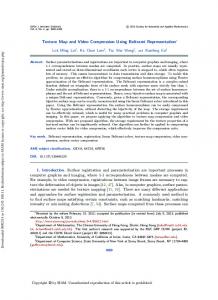
Fig. 1. Two-dimensional example of selectively transmitting coefficients belonging to region of interest (the shaded regions approximate the important coefficients).
Considering decomposition along the temporal direction, the application of the wavelet transform to a signal segment results in two lower resolution component segments (the lowpass and the highpass). Now, it is in our interest that the pixels of the frames that we wish to code, when wavelet transformed, end up in a confined region and not have their effect dispersed among too many coefficients in the transform domain. The reason for this is that we are going to extract the wavelet frames, and hence we would coefficients concerning the last not want these to be too many, otherwise we would have low coding efficiency. Not all wavelets have such a characteristic as will be explained later in this section. Fig. 1 shows a schematic diagram for an example of what is meant by having a signal effect confined when wavelet transformed. It is easier to comprehend this 2-D version, and the 3-D version follows easily. In the figure, we assume new columns (as that we have a 2-D signal with opposed to frames). Now we wish to transform the 2-D signal concerning the new columns but by applying a transform to
KHALIL et al.: 3-D VIDEO COMPRESSION
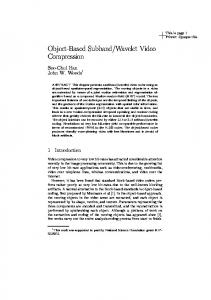
the whole signal to make use of any correlation. After the second iteration, the coefficients concerning the new columns will be dispersed as shown in the shaded regions in the figure. Now we want to transmit only the coefficients in the shaded parts. At the other end, the receiver has in its buffer only the old columns. Now before we can inverse transform the coefficients concerning the new columns that the receiver has just received, we would like to insert them in their correct respective places. Before we can do that, the receiver must wavelet transform the old columns and since the dimensions of the 2-D image must be equal to that at the transmitter, assumed columns we will extend the 2-D old columns by (chosen, for example, as a constant extrapolation of the last frame). Now we transform this extended signal, and reinsert the coefficients that the transmitter sent in their corresponding places. The process of inserting the coefficients into their respective places replaces the coefficients that result from the assumed columns. In reality, the transformation causes wider dispersion than shown in the shaded regions. We only transmit the more important coefficients, since it will not be cost-effective to transmit the remaining coefficients from the compression point-of-view. Due to neglecting coefficients, this approximation becomes more and more accurate when the new frames are more correlated with the old frames. Practical experiments (Section V) show that it is an acceptable approximation in general, especially if movement in the video is slow, as is the case in typical video-conferencing-type sequences. After such a procedure, we will now end up with a 2-D signal that resembles the original 2-D signal that we are compressing. In other words, even though we coded a few columns, we were able to take into account the correlation over a wider range of columns while not sacrificing extra bit rate. A 3-D interpretation follows easily, and Fig. 2 offers an example concerning four new frames that are to be coded. Two decomposition iterations are performed. It remains to be seen if there exist filters that when applied to a signal segment will not disperse the effect of a localized region. If, for example, we consider the 9-tap QMF filter, a single pixel in a signal segment will affect a total of coefficient. If we want perfect reconstruction, then all 17 coefficients concerning this one pixel must be transmitted to the receiver. This figure, in fact, is lower than 17 because, first we are not treating one pixel but four adjacent pixels and then there would be overlap in the affected coefficients, and second we are treating pixels at the edge of a signal segment, and that we ignore affected regions that are outside our scope. But then, the figure is still too high, and it would be advantageous to find a filter that has approximately four coefficients affected by four pixels. Such a setup can be achieved if we use the Daubechies’ filters [13] because it has a more compact representation. When we specifically use the 6-tap filter, which was built to allow perfect reconstruction, we find that the influence of a group of pixels in a signal segment is still a bit too wide (dispersion still occurs). Therefore, we make an approximation by neglecting the least affected of these dispersed coefficients. Retaining all affected coefficients is the only way to ensure perfect reconstruction, but this is inefficient. A cost-effective
765
Fig. 2. Cubic portion of frames undergoing 3-D wavelet transformation. Notice the position of the coefficients that depend on the last four frames.
solution, that we found to give acceptable distortion, is to retain as many coefficients as there were pixels and neglect the rest. A heuristic choice of retained coefficients is shown in Figs. 1 and 2, and these coefficients are the most dependent on the pixels that we want to compress. It is important to note that in general, filter-length does not directly affect the time-locality. We just stress that in the special circumstances of this algorithm, where coefficients are neglected in this special way, filters may in fact have different characteristics, especially when handling signals at regions near the edges. We have performed experiments and the results agree with this symmetric interpretation. In the spatial domain, we use the QMF filters because they have superior performance, and the circumstances allow us to use them. A. Detailed Steps of the Algorithm Step 1: When the transmitter and receiver start to make contact, the transmitter sends 12 frames using any kind of coding. We suggest a sort of intraframe coding for simplicity. The lowpass coarsest subband is coded using adaptive Huffman coding with past frame prediction. These 12 frames will be the basis of our prediction in the 3-D transform.
766
Step 2: The transmitter buffers new frames. old Step 3: The transmitter now having frames, and new frames, i.e., a total of 16 frames, can perform a 3-D decomposition of the signal. To make practical implementation possible, we divide the frames into spatial blocks of size 64, such that the 3-D signal that we will 64 64 handle at any one time is of dimensions 64 16. Step 4: The encoder at the transmitter, must now locate the coefficients in the transform domain that depend frames. Their (or depend most) on the positions are usually known beforehand and are fixed for any set of filters (see Fig. 2). These coefficients are then coded using any efficient coding method. We describe one such method later in this section. Step 5: Now the receiver has already 12 old frames, and new frames. But needs to reproduce the these 12 old frames are not in the transform domain, while the data received from the transmitter is. We then extend the 12 frames to 16 by repeating the 12th frame four times. Then we 3-D transform such a 64 64 16 signal. We then receive the coded coefficients corresponding to the four new frames, and distribute them among their correct locations. When we distribute these coefficients among their locations, they will approximately replace all the coefficients concerning the extended four frames. 64 16 Step 6: Now that the receiver has a 64 block that resembles the original one except for quantization errors, we can perform an inverse 3-D wavelet transform to the block and end up with our 12 old frames plus the four new frames. Step 7: This process is first repeated for all spatial 64 64 blocks. When we have completed the whole frame size, the receiver and transmitter can now shift back in time the frames by four temporal locations to get ready for another four new frames. We then return to step 2. As we see in step 5 above, the receiver extends the number of frames to 16 by repetition before applying the temporal decomposition. As mentioned earlier, the coefficients representing these frames will be a little dispersed beyond the confinement region. We are only able to replace some of them when we distribute the coefficients that are received from the transmitter. Because it was found to be cost-effective only to send the more important coefficients, there will be some mismatch between the transmitter and the receiver. To solve this potential problem, the transmitter repeats all steps undertaken by the receiver. In other words, the transmitter, after it has selected the coefficients to be sent (and quantized them), performs a four-frame extension by repetition, then forward transforms the 3-D block, reinserts these coefficients and then performs a backward transform. Now, both receiver and transmitter are ensured to be in full synchronism.
IEEE TRANSACTIONS ON IMAGE PROCESSING, VOL. 8, NO. 6, JUNE 1999
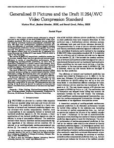
Fig. 3. Parent-child relationship for a 3-D version of zero-trees for a two-level decomposition of 3-D signal.
IV. THREE–DIMENSIONAL ZERO-TREE CODING The performance of any codec not only depends on the choice of wavelet filter or the number of decompositions, but also on the way the coefficients are quantized and encoded. Many successful 2-D wavelet-based image compression schemes have been reported in the literature, ranging from simple entropy coding to more complex techniques such as vector quantization [12], tree encodings [15], [16], and edgebased coding [17]. Shapiro’s zero-tree [15] encoding algorithm defines a data structure called a zero-tree. An extension to this algorithm to suit 3-D coding was derived independently in [25] prior to the appearance of [4]. This section briefly outlines the major concepts of a 3-D zero-tree coding algorithm, and how it is used to fulfill our objective. is first filtered along the The image sequence dimension, resulting in a lowpass image and a . Since the bandwidth of and highpass image along the dimension is now half that of , we can safely downsample each of the filtered image sequences in dimension by two without loss of information. The the downsampling is accomplished by dropping every other filand are then filtered along the tered value. Both dimension, resulting in four subimage sequences: , and . Once again, we can downsample the subimages by two, this time along the dimension. Then each of these four subimage sequences are then filtered along the dimension, resulting in eight subimages: , and (see Fig. 3). The 3D filtering decomposes an image sequence into the slowly and seven detail signals which moving average signal emphasizes are directionally sensitive: for example, slowly changing the quickly changing average signal, horizontal image features, the slowly changing vertical the quickly changing diagonal features. features, and
KHALIL et al.: 3-D VIDEO COMPRESSION
The directional sensitivity of the detail signals is caused by the frequency ranges they contain. It is common in wavelet compression to recursively trans. The number of transformaform the average signal tions performed depends on several factors, including the amount of compression desired, the size of the original image, and the length of the filters. In general, the higher the desired compression ratio, the more times the transform is performed. The encoder/decoder pair, or codec, has the task of compressing and decompressing the sparse matrix of quantized coefficients. A wavelet coefficient is said to be insignificant . The zero-tree with respect to a given threshold if is based on the assumption that when a wavelet coefficient at a coarse scale is insignificant with respect to some threshold , then all wavelet coefficients having the same orientation (as defined by the type of filters applied to any one subband) at the same spatial and temporal location at all finer scales (lower decomposition levels) are likely to be also insignificant with respect to . Consider a hierarchical recursive wavelet system. We define parent and child relationships to relate coefficients of one given scale to the next. The first modification to make is the zero-tree shape. In 2-D, a zero-tree starts as a single coefficient child coefficients, then each of those then it has another four, and so on. In three dimensions, a zero-tree starts as a single coefficient. Then, for the next level, it will have child coefficients, each of which has another eight, and so on. If we are assuming a two-level decomposition then the parent/child relationships are as follows (see Fig. 3): A coefficient in LLH2 is the parent of eight coefficients in LLH1 (where one and two are the first and second decomposition levels, respectively). A coefficient in LLH1 has no children. A coefficient in HLL2 is the parent of eight coefficients in HLL1 and so on. When encoding the zero-tree information, a scanning of the coefficients is performed in such a way that no child node is scanned before its parent. For an -scale transform, the scan is done separately for each of the slowly, and the quickly moving subbands. The slowly moving subband scan, for example, begins at the lowest frequency subband, denoted , and scans subbands , and , by , etc. Note that at which point it moves on to scale each coefficient within a given subband is scanned before any coefficient in the next subband. A coefficient is said to be an element of a zero-tree for if itself and all of its descendants (children a threshold and children of children and so on) are insignificant with respect to . A symbol is used to indicate a zero-tree root and the insignificance of the coefficients at all finer scales. This information can be efficiently represented by a string of symbols from a three-symbol alphabet (similar to [15]) which can be entropy-coded. These three symbols are 1) zerotree root (ZT), 2) isolated zero (IZ), which means that the coefficient is insignificant but has some significant descendent, and 3) significant (SIG). It has also been found more efficient to encode runs of zero-tree root symbol (ZT) using variable codeword-length run-length encoding. A state diagram is shown in Fig. 4. Thus
767
Fig. 4. State diagram showing possible output sequences.
we are always in one of two states: we are either counting runs of ZT, or we encode either IZ or SIG. We chose that we alternate between the two states so as to save on the signaling requirement that would be needed to switch also between IZ and SIG (more efficient to inhibit transition between IZ and SIG, and provide a run-length of zero of ZT in exchange). ZT run-length values are encoded using fixed Huffman tables as in [18]. Formerly marked descendants of a previously found zero-tree root are not counted in the run-length as they are known at the decoder. To differentiate between IZ or SIG, we use one bit. In case the coefficient is SIG, we quantize the coefficient using a nonlinear optimal Lloyd quantizer and then entropy-encode the quantized values. As for the lowest subband (the one subjected only to lowpass filters), we code it using variable length differential pulse code modulation (DPCM) with past frame prediction. Fixed Huffman tables are used to encode differential values as the distribution of differential values is a priori known. V. CODING RESULTS In this section, we demonstrate the performance of the proposed system. We use the first 36 frames of the image 256 sequences Claire and salesman. We only use a 320 64 portion of the frame so as to simplify division into 64 blocks. The frame rate is 30 frames/s, and we handle the gray-scale frames, which have a resolution of 256 levels. As indicated before, we code the first 12 frames using 2-D coding, then we switch to 3-D coding mode. The PSNR of the different frames for the Claire and salesman sequences are indicated in Figs. 5 and 6, respectively. Shown in these figures are comparisons of the ITU-T H.261 [19] standard and the 3-D wavelet systems that use the Haar wavelet and the six-tap Daubechies filter. Coding of the first 12 frames for the 3-D methods requires an average bit rate of around 900 kb/s. The steady-state bit rate for all designs is fixed around 300 kb/s. Results are demonstrated only for the 256 portion of the sequences and the following peak 320 signal-to–noise ratio (PSNR’s) are calculated as averages of frame 13 to frame 36, because that is when all sequences are running at the same bit rate. The average PSNR over the test sequence Claire for H.261 is 40.58 dB, for Haar is 40.05 dB, and for 6-tap Daubechies is 40.63 dB. The
768
Fig. 5. PSNR comparison of Claire sequence. Two-dimensional coding is used till frame 12, then 3-D afterwards.
Fig. 6. PSNR comparison of salesman sequence. Two-dimensional coding is used till frame 12, then 3-D afterwards.
average PSNR over the test sequence salesman for H.261 is 35.58 dB, for Haar is 35.48 dB, and for 6-tap Daubechies is 35.97 dB. This shows that incorporating as many frames as possible in the decomposition (6-tap Daubechies versus Haar) produces better results, and the performance of this new system is comparable to H.261, if not better. But this design does not require the time and computation consuming motion compensation (MC) step and thus can be viewed as a better solution in situations where such resources are scarce. However, standards like H.261 and H.263 [20] have quite sophisticated MC procedures that are the main source of their efficiency. H.263 outperforms H.261 by about 2 dB for these sequences, and the main source of this additional improvement is mainly attributed to further improvements in MC. H.263 is a highly optimized method and is therefore very hard to beat. In our proposed wavelet approach, we have not used any MC, so in that sense our results are favorable. Recent work in [21]–[23] combined MC with 3-D subband coding and very promising results were demonstrated. We believe that if our proposed system outperforms H.261 in its present state, then adding H.261’s MC will most probably improve performance, and such complicated MC as used in H.263 even more. This reduced-buffering 3-D codec can approximate a real 3-D codec only under conditions that neglected coefficients are in fact negligible. Under conditions of high-motion, we expect these
IEEE TRANSACTIONS ON IMAGE PROCESSING, VOL. 8, NO. 6, JUNE 1999
Fig. 7. PSNR comparison of Claire sequence at 64 kb/s.
coefficients to be more significant and the codec performance is bound to deteriorate. It becomes necessary to have motioncompensation to counteract any motion that occurs. Any discrete cosine transform based (DCT-based) codec will suffer similar fate when no motion-compensation is used. Many of the referenced papers on 3-D coders show compression results that are favorable when motion is low, then significant drops in PSNR are exhibited when motion increases. Research is under way in combining the MC step of [21] to our proposed method, but this will be studied in a future work. Also, though zerotree encoding is a very effective coding technique, it can easily be exchanged with any other more effective coding technique that is discovered in the future. The actual encoding of the wavelet coefficients and the actual way that the system works are two separate issues. We also conducted a test at the lower rate of 64 kb/s. Fig. 7 shows the results for the Claire sequence. The average PSNR for the 3-D codec is 36.82 dB and that of the DCT based system is 36.78 dB. To achieve the shown results, we code CIF frames at only 10 frames/s. Subjectively, the 3-D wavelet codec produced reconstructed frames that did not contain blocking degradations that are always produced in H.261. The blurring that occurred in high movement areas were not as annoying as these blocking effects. See Fig. 8 for a comparison of the H.261 output with that of our 3-D coder for the Claire sequence for the higher bit rate (frame 33), and Fig. 9 for the lower bit rate (frame 90). The thirty-third frame, for the lower rate, was chosen on purpose to show that even when the PSNR of the 3-D coder is lower than H.261 for that particular frame, the subjective results are favorable. The performance of our coder is more pronounced when movement is low since we do not use MC as previously explained. This can be noticed in the second part of the salesman sequence where movement is low. Fig. 10 shows a comparison of the thirty-sixth frame of salesman. One final comment about the results is that the quantitative periodic change in PSNR that is seen in Figs. 5–7, is a problem that is characteristic of most 3-D subband/wavelet coders reported in the literature. It is mainly due to the fact that the joint encoding of a group of frames makes it difficult to know which coefficients affect exactly which frames, since it is considered now a 3-D signal, i.e., a single unit.
KHALIL et al.: 3-D VIDEO COMPRESSION
(a)
(b)
769
(a)
(b)
(c) Fig. 8. Comparison of thirty-third frame of Claire sequence. (a) Original. (b) H.261. (c) Three-dimensional coder (6-tap Daubechies).
It is interesting to study how the codec would perform at higher bit rates. As mentioned before, the 3-D decomposition causes dispersion of coefficients that concern the frames that we wish to encode. Because we neglect some coefficients
(c) Fig. 9. Comparison of ninetieth frame of Claire sequence at 64 kb/s. (a) Original. (b) H.261. (c) Three-dimensional coder (6-tap Daubechies).
in the way we code them, that places an upper limit on possible reconstruction performance. We have conducted tests on both the Claire sequence and the salesman sequence under
770
IEEE TRANSACTIONS ON IMAGE PROCESSING, VOL. 8, NO. 6, JUNE 1999
Fig. 11. Performance of the 3-D codec under conditions of “No quantization” of the 3-D coefficients. Frames 1–12 have exact reconstruction as they are unaffected by neglected coefficients. (a)
(b)
(c) Fig. 10. Comparison of thirty-sixth frame of salesman sequence. (a) Original. (b) H.261. (c) Three-dimensional coder (6-tap Daubechies).
conditions of no quantization. Fig. 11 shows the output results. It can be seen that the neglected coefficients do have an
impact on the highest achievable PSNR. So even if bit rate is available, performance is bounded by the curves shown in the graph. To overcome this limitation, we must use a different coefficient encoding algorithm (different from the used zerotree) because the zero-tree codes all coefficients in the same manner irrespective of the subband. In a modified algorithm, we would need to distribute the available bit budget in a more intelligent way. Enhancements to the performance of the coding algorithm are also possible. As indicated in the procedure, it is seen that a 3-D forward and backward wavelet transform is performed for frames, while we are indeed only concerned about all . The following three steps can considerably decrease the required computations: 1) The first step addresses the issue of the forward transform at the transmitter. Since the transmitter will only send selected coefficients (those concerned only with the new frames), then we can perform the forward wavelet transform only for the needed coefficients and save considerable time. 2) The second step concerns the forward transform at the receiver. If we consider the decomposition along the temporal axis, it should be noted that most of the coefficients calculated using convolution with the analysis filters correspond exactly with a translated counterpart from the transformed 3-D block that we handled when we were considering the previous four frames. Thus for those coefficients, we need only perform a translation of the coefficients from the previous forward transformed block. The quantity of such translation depends on the specific coefficient. If the coefficient is in the first decomposition level, then we translate it by positions back in the temporal direction. If it is the second decomposition level, then we shift it by positions, and so on. 3) Since at the receiver, we are only concerned with calculating the pixels inside the four new frames, we thus only inverse transform such pixels. The overall effect of these optimizations is a decrease of the required computations, at the cost of a slightly more
KHALIL et al.: 3-D VIDEO COMPRESSION
771
sophisticated implementation, but the purpose is to show that frames as part of a larger frames does not treating necessarily constitute a proportional increase in computations.
Scheme B Another possible implementation for the forward and backward transform is as follows:
VI. CONCLUSION
(7)
A 3-D coding system for video conferencing applications has been introduced. 3-D coding for such applications was usually avoided because of the delay that such a system would introduce. A method whereby advantages of 3-D coding can be effectively made use of was demonstrated, and a solution to the delay problem was highlighted. Although the proposed algorithm is comparable to the H.261 standard and worse that the H.263 standard, it has the advantage of lower computational complexity. In addition, by adding the sophisticated MC of H.261 or H.263, performance of the developed algorithm can be further enhanced. We believe there is room for improvement in this direction, but this will be studied in a future work. APPENDIX Because the forward and backward transformations are accomplished by a convolution operation, we run into the problem of edge-effects. For the Daubechies family of filters (which are nonsymmetric filters), there exists only one simple edge extension solution that involves cyclically repeating the signal to form an infinite-like signal. When quantizing coefficients resulting from transforming such a signal, high reconstruction errors may appear, especially if the signal has highly differing amplitudes at the opposing edges. Here, we present a new edge-extension that has better performance under general circumstances. Before we describe the new edge-extension, we will explain why exactly the finite-length input signal poses a problem. Application of the forward and backward transforms can be implemented in several different ways. We present here two schemes: Scheme A This is the same as described in Section II; it is repeated here for convenience. The forward transform can be performed as follows:
(8)
(9) Both Scheme A and Scheme B suffer from edge-problems. Scheme A gives perfect reconstruction at the right edge, but distorts the left edge. As can be seen from (4) and (5), the analysis accesses elements (beyond the right edge) and the synthesis accesses elements (beyond the left edge). In the analysis cycle, we can make any arbitrary extension and would still obtain perfect reconstruction at the right edge. In the synthesis cycle, however, not just any extension at the left edge will lead to perfect reconstruction. Scheme B has the same problems except that the edges are switched, and now only the left edge gets perfect reconstruction. Since Scheme A and Scheme B are very similar, only Scheme A will be discussed in detail. Now, the problem can be solved if we can extend the left edges of and so that the analysis cycle can be performed. We can force perfect reconstruction at the left edge by making some suitable , and beyond their left edge such extension to the signal that over an analysis and then synthesis cycle at that edge, we will get exact reconstruction for all edge pixels. This, however, will not work using (4), (5), and (6) as they are. To see this, note that (4) and (5) do not even access elements below . This means extending the signal at the left edge seems worthless. Even if we use equations of Scheme B, the exact same situation occurs. We propose, therefore, to solve this other problem by implementing the analysis/synthesis as the following scheme. Scheme C
(4) (10) (5) (11) is the where represents the lowpass downsampled result, highpass downsampled result, and and respectively are the and . The coefficients of the discrete-time forward filters backward transform is performed as follows:
(12)
(6)
Here, it must be noted that the forward transform, denoted by (10) and (11), now requires the knowledge of both the sigand nal elements (i.e., requires extension at both edges). The backward trans-
772
IEEE TRANSACTIONS ON IMAGE PROCESSING, VOL. 8, NO. 6, JUNE 1999
form now needs to extend to the left and to the right. This now is very appropriate because now we can achieve perfect reconstruction at both edges by choosing those edgeextensions wisely. We will only demonstrate the solution for the left edge and the analysis will carry over to the case of the right edge. As mentioned before, we need to extend the signal at the left edge (and right edge), and the signal to the left. Denote , those extended elements of the signal : , respectively. Also denote the extended by ( is always elements of the signal : , respectively. From an even number), by the analysis and synthesis equations (10)–(12), we can obtain linear equations that give the reconstruction values at the edge elements of the signal. In other words, we can write as a linear combination of terms of , and as a linear combination of terms of , which will now include terms depending on . Then we write the reconstruction linear in terms of both and , but also equations that give . Since now is in terms of both and (and ), then it would also be in terms of (and ). Now if we impose to exactly match , we get a linear equation with only and unknown. Now if we get a set of such equations for different , we will get a set of linear simultaneous equations that can and . Because we only have be solved for the unknowns equations that actually reference and , and the fact unknowns, we have the that we have a total of variables freedom to assume the values of a total of and still be able to find perfect solutions to the equations. One such set of assumed values may be to mirror-reflect , . This such that unknowns and was found to perform makes up for well under quantization. Thus, now we only have to solve for the unknowns . With some simple manipulation of these equations, we can write (13) where (14) and (15) . where is a constant matrix of dimensions elements of follows from The reason why we need careful examination of (10)–(12). After we have found such a matrix , it can be fixed for any Daubechies filter. Thus, solving the simultaneous equations is all done off-line to calculate the matrix . During online operation of the transformation step, all we do is just mirrorreflection for the extension of and calculate (13) and use as the extension for . Thus, this edge extension scheme is not complex to implement and involves a simple matrix multiplication at the edge of the signal segment. We repeat this similarly for the right edge. We wish to note another interesting solution for the edgeeffect problem that has recently been developed [24]. The
solution was based on the idea that since the Daubechies vanishing moments, it can represent tap filter has very efficiently. Then if a polynomial of degree it is assumed that the extension of the finite length signal segment is the coefficients of a polynomial of such a degree, a polynomial expansion of the scaling function around the region will produce a number of linear equations that can be solved to deduce these coefficients.
REFERENCES [1] D. Taubman and A. Zakhor, “Multirate 3-D subband coding of video,” IEEE Trans. Image Processing, vol. 3, pp. 572–588, Sept. 1994. [2] Y. K. Kim, R. C. Kim, and S. U. Lee, “On the adaptive 3D subband video coding,” in Proc. SPIE, vol. 2727, pp. 1302–1312, Mar. 1993. [3] A. Mainguy and L. Wang, “Performance analysis of 3-D subband coding for low bit rate video,” in Proc. SPIE, vol. 2952, pp. 372–379, 1996. [4] Y. Chen and W. Pearlman, “Three-dimensional subband coding of video using the zero-tree method,” in Proc. SPIE, vol. 2727, pp. 1302–1312, Mar. 1997. [5] E. Chang and A. Zakhor, “Scalable video coding using 3-D subband velocity coding and multirate quantization,” in Proc. Int. Conf. Acoustics, Speech, and Signal Processing, Minneapolis, MN, Apr. 1993, vol. 5, pp. 574–577. [6] G. Karlsson and M. Vetterli, “Three dimensional subband coding of video,” in Proc. ICASSP, 1988, pp. 1100–1103. [7] C. I. Podilchuk, N. S. Jayant, and N. Farvardin, “Three-dimensional subband coding of video,” IEEE Trans. Image Processing, vol. 4, pp. 125–139, Feb. 1995. [8] M. Domanski and R. Swierczynski, “Efficient 3-D subband coding of color video,” in Proc. IWISP’96, Manchester, U.K., pp. 277–280. [9] T. Alonso M. Luo, H. Shahri, and D. Youtkus, “3D subband coding of video conference sequences,” in Proc. Int. Conf. Signal Processing Applications and Technology, Dallas, TX, Oct. 1994, vol. 2, pp. 933–938. [10] S. Mallat, “A theory for multiresolution signal decomposition: The wavelet representation,” IEEE Trans. Pattern Anal. Machine Intell., vol. 11, pp. 674–693, July 1989. [11] G. Karlsson and M. Vetterli, “Extension of finite length signals for subband coding,” Signal Process., vol. 17, pp. 161–166, June 1989. [12] M. Antonini, M. Barlaud, P. Mathieu, and I. Daubechies, “Image coding using wavelet transform,” IEEE Trans. Image Processing, vol. 1, pp. 205–220, Apr. 1992. [13] Y. Chan, Wavelets Basics. Boston, MA: Kluwer, 1995. [14] I. Daubechies, “Orthonormal bases of compactly supported wavelets,” Commun. Pure Appl. Math., vol. 41, pp. 909–996, Nov. 1988. [15] J. Shapiro, “Embedded image coding using zerotrees of wavelet coefficients,” IEEE Trans. Signal Processing, vol. 41, pp. 3445–3462, Dec. 1993. [16] A. Lewis and G. Knowles, “Image compression using the 2-d wavelet transform,” IEEE Trans. Image Processing, vol. 1, pp. 244–250, 1992. [17] J. Froment and S. Mallat, “Second generation compact image coding with wavelets,” Wavelets: A Tutorial and Applications. New York: Academic, San Diego, CA, vol. 2, pp. 655–678, 1992. [18] G. Einarsson, “An improved implementation of predictive coding compression,” IEEE Trans. Commun., vol. 39, pp. 169–171, Feb. 1991. [19] ITU-T Recommendation H.261, “Video codec for audiovisual services at p 64 kbits/s,” Dec. 1990, Mar. 1993. [20] ITU-T Recommendation H.263, “Video coding for low bit rate communication,” Dec. 1995. [21] J.-R. Ohm, “Three-dimensional subband coding with motion compensation,” IEEE Trans. Image Processing, vol. 3, pp. 559–571, Sept. 1994. [22] P. Waldemar, M. Rauth, and T. A. Ramstad, “Video compression by three-dimensional motion-compensated subband coding,” in Proc. Norwegian Signal Processing Symp., pp. 227–232, Sept. 1995. [23] K. Ngan and W. Chooi, “Very low bit rate video coding using 3D subband approach,” IEEE Trans. Circuits Syst. Video Technol., vol. 4, pp. 309–316, June 1994. [24] J. Williams and K. Amaratunga, “A discrete wavelet transform without edge effects using wavelet extrapolation,” IESL MIT Tech. Rep., 95-02, Jan. 1995. [25] H. Khalil, “New coding techniques for video images in conferencing applications,” M.Sc. thesis, Cairo Univ., Cairo, Egypt, 1996.
2
KHALIL et al.: 3-D VIDEO COMPRESSION
Hosam Khalil (S’98) was born in Washington, DC, in 1972. He received the B.S. and M.S. degrees in electrical engineering with honors from Cairo University, Cairo, Egypt, in 1993 and 1996, respectively. He is currently pursuing the Ph.D. degree at the University of California, Santa Barbara. From October 1993 to July 1996, he was an Assistant Teacher at Cairo University. He was also employed part-time during that period with IBM, Egypt. In the summer of 1998, he was an intern in the Multimedia Communications Research Laboratory, Bell Laboratories, Murray Hill, NJ. His research interests are in image and speech compression and recognition. Mr. Khalil was a recipient of the UC Regents Fellowship.
Amir F. Atiya (S’86–M’90–SM’97) was born in Cairo, Egypt, in 1960. He received the B.S. degree in 1982 from Cairo University, and the M.S. and Ph.D. degrees in 1986 and 1991 from the California Institute of Technology (Caltech), Pasadena, CA, all in electrical engineering. From 1985 to 1990, he was a Teaching and Research Assistant at Caltech. From September 1990 to July 1991, he held a Research Associate position at Texas A&M University, College Station. From July 1991 to February 1993, he was a Senior Research Scientist at QANTXX, Houston, TX, a financial modeling firm. In March 1993, he joined the Computer Engineering Department, Cairo University as an Assistant Professor. He spent the summer of 1993 with Tradelink Inc., Chicago, IL, and the summers of 1994, 1995, and 1996 with Caltech. In March 1997, he joined Caltech as a Visiting Associate in the Department of Electrical Engineering. In January 1998, he joined Simplex Risk Management Inc., Hong Kong, as a Research Scientist, and he is currently holding this position jointly with his position at Caltech. His research interests are in the areas of neural networks, learning theory, pattern recognition, data compression, and optimization theory. He has published about 60 papers in these fields. His most recent interests are the application of learning theory and computational methods to finance. Dr. Atiya received the Egyptian State Prize for Best Research in Science and Engineering in 1994. He also received the Young Investigator Award from the International Neural Network Society in 1996. Currently, he is an Associate Editor for the IEEE TRANSACTIONS ON NEURAL NETWORKS. He served on the organizing and program committees of several conferences, most recently Computational Finance, New York, 1999, and IDEAL’98, Hong Kong.
773
Samir I. Shaheen (S’74–M’81) received the B.Sc. and M.Sc. degrees from the Department of Electronic and Communications Engineering at Cairo University, Cairo, Egypt, in 1971 and 1974, respectively, and the Ph.D. degree from McGill University, Montreal, P.Q., Canada, in 1979. From 1979 to 1981, he worked in Computer Vision Laboratory, McGill University. In 1981, he joined Cairo University as an Assistant Professor. He joined the Computer Science Department, King Abdulaziz University, Saudi Arabia, as a Visiting Professor. He is currently a Professor in the Computer Engineering Department, Cairo University, and Director of the Computer Laboratories. He is the Manager of Cairo University Computer Network and Computer Research Center. His current research interests include neural networks, medical imaging, document analysis, and multimedia in high speed digital networks.