In fact, most propositional formulas have exponentially sized BDDs [27]. To cope with such systems, bounded model checking (BMC) has been proposed as an ...
Three–Valued Logic in Bounded Model Checking Tobias Schuele and Klaus Schneider Reactive Systems Group, Department of Computer Science, University of Kaiserslautern P.O. Box 3049, 67653 Kaiserslautern, Germany {Tobias.Schuele,Klaus.Schneider}@informatik.uni-kl.de http://rsg.informatik.uni-kl.de
Abstract In principle, bounded model checking (BMC) leads to semidecision procedures that can be used to verify liveness properties and to falsify safety properties. If the procedures fail, there is usually no information about the validity of the considered specification. In this paper, we present a new approach to BMC based on three-valued logic that allows us in many cases to falsify liveness properties and to verify safety properties. Moreover, we employ both global and local model checking to take advantage of the different types of specifications that can be handled by these techniques.
1. Introduction In the past two decades, model checking has evolved as one of the main technologies for the verification of reactive systems. The system to be verified is thereby given as a transition system with finitely or infinitely many states, and the specifications as formulas that refer to the states or paths of the transition system. Many formalisms like temporal and predicate logics, sequence diagrams, finite automata, and others have been considered for that purpose [16, 29]. It turned out, however, that most of these formalisms are subsumed by the µ-calculus. As a result, the design of verification systems can be split into frontends that translate specifications to µ-calculus model checking problems, and backends that solve these problems. Hence, the main effort for improving the efficiency of verification should focus on µ-calculus properties. The success of model checking is to a large extent due to efficient set representations by means of characteristic functions. In particular, binary decision diagrams (BDDs) [12] have been successfully used for the representation of large sets and coined the notion of symbolic model checking. In the same way as finite sets can be represented by BDDs, finite automata have been proposed as generalizations of BDDs for the representation of infinite sets [2, 7, 8].
0-7803-9227-2/05/$20.00 ©2005 IEEE
On the one hand, BDDs often allow the verification of very large systems, but on the other hand, they may fail for relatively small systems. In fact, most propositional formulas have exponentially sized BDDs [27]. To cope with such systems, bounded model checking (BMC) has been proposed as an alternative to symbolic model checking [4, 5, 6, 15, 17, 33, 34]. The main idea of BMC is to reduce the model checking problem to a satisfiability problem of the underlying base logic. In principle, this is accomplished by limiting the number of fixpoint iterations according to an a priori estimated bound. In this way, fixpoint formulas can be syntactically replaced with finitely many approximations obtained by unwinding the formulas. The resulting formulas can then be checked using sophisticated SAT solvers. However, bounded model checking as described above can only be used to disprove, but not to prove greatest fixpoint formulas. This is due to the fact that greatest fixpoint formulas are computed by successively removing states until the fixpoint is reached. If one of the initial states is not contained in an approximation, the specification is disproved. Otherwise, nothing can be said about the validity of the specification, since the final fixpoint is not known. Analogously, least fixpoints can be proved, but they cannot be disproved: The computation of least fixpoints starts with the empty set and iteratively adds states to refine the approximations. If the initial states are included in an approximation, the specification is proved. Otherwise, it is not clear whether the specification holds. Bounded model checking is an active area of research, and many improvements have been developed in recent years. One approach to obtain complete decision procedures is to determine a maximal bound for unwinding the specification which is called the completeness threshold. Given a bound that is greater than or equal to the completeness threshold, BMC is complete for finite systems [17, 5]. Another approach is loop detection, a technique to detect cycles in the transition system [4, 6, 15]. However, this often increases the size of the resulting formulas significantly and slows down the verification process.
166
Authorized licensed use limited to: Technische Universitat Kaiserslautern. Downloaded on March 12, 2009 at 07:22 from IEEE Xplore. Restrictions apply.
For systems with infinitely many states the situation is even worse. First, there is generally no completeness threshold, and hence, completeness of the model checking algorithms cannot be achieved by choosing a sufficiently large bound. Second, there may exist infinite paths that do not contain loops. Thus, loop detection fails for such paths. In this paper, we propose the use of three-valued logic for bounded model checking to solve these problems. The idea of our approach is to explicitly state the fact that some properties are not known. In particular, the characteristic functions of state sets, which are traditionally Boolean functions, now become three-valued functions. If for such a function λ and an element x, the value λ(x) is true, we know that x belongs to the set represented by λ. Conversely, if λ(x) is false, then x does not belong to the set represented by λ. Finally, if λ(x) yields the third value denoted as ⊥, there is no information about the membership of x. Moreover, we present a bounded version of local model checking (LMC) [9, 10, 18, 38, 39]. In contrast to global model checking (GMC) that relies on fixpoint computation, LMC is based on the construction of proof trees using syntax directed decomposition rules. There are many differences between these two approaches, e.g. the way a formula is evaluated: In GMC, the syntax tree of a specification is traversed in a bottom-up manner, whereas in LMC, a specification is evaluated top-down. However, the most important difference is that GMC is based on fixpoint iteration as mentioned above, while LMC follows an inductive style of reasoning. Hence, bounded local model checking (BLMC) can be viewed as a generalization of methods that integrate induction in bounded model checking [19, 20, 21, 36]. In [35] it was shown that global and local model checking procedures are incomparable for the verification of infinite state systems. In other words, some specifications can be proved by GMC, but not by LMC, and vice versa. To obtain more powerful verification algorithms, we present a combination of both approaches. Again, the key to keep track of positive, negative, and uncertain information is the use of three-valued logic. In this way, a large class of specifications can be checked automatically. Multi-valued logics have already been used in model checking to analyze models that contain uncertain or inconsistent information. In [22, 23], Fitting introduced the notion of multi-valued models and explored appropriate extensions of modal logics to reason over such models. Some years later, Bruns and Godefroid investigated three-valued model checking of partial Kripke structures [11]. A more general approach is presented in [14], where both atomic propositions and transitions between states may take a truth value of a given multi-valued logic. In contrast to these approaches, our work leverages three-valued logic to increase the power of the model checking algorithms while retaining the model and the specification.
The rest of this paper is organized as follows: In the next section, we explain the foundations of the µ-calculus and briefly discuss global, local, and bounded model checking. Moreover, we describe the basics of three-valued logic. In Section 3, we present bounded versions of global and local model checking using three-valued logic. Additionally, we show how these approaches can be combined. Finally, we conclude with a summary and directions for future work.
2. Foundations 2.1. µ-Calculus In the following, we use the µ-calculus to reason about the temporal properties of reactive systems. As mentioned previously, the µ-calculus subsumes popular temporal logics like CTL and LTL [29]. This allows us to deal with a larger class of specifications compared to previous work on BMC that is usually based on LTL. However, the µ-calculus does not provide any means for reasoning about atomic properties of a system, it rather serves as an extension of a given base logic. In principle, every logic L can be extended to a corresponding temporal logic Lµ by adding fixpoint and modal operators as follows: Definition 1 (Syntax of the µ-Calculus) Given a logic L and a set of Boolean variables V B , the set of µ-calculus formulas Lµ is defined as follows with α ∈ L, ϕ, ψ ∈ Lµ , and Z ∈ V B : − ← − ← Lµ := α | Z | ϕ ∧ ψ | ϕ ∨ ψ | �ϕ | ♦ϕ | � ϕ | ♦ ϕ | µZ.ϕ | νZ.ϕ The set of modal formulas, i.e., the set of formulas that do not contain fixpoint operators, is denoted by L� . Models of µ-calculus formulas are transition systems whose states correspond with interpretations of the base logic L. The transition systems are also called Kripke structures due to the relationship to modal logics. Definition 2 (Kripke Structure) A Kripke structure K = (S, I, R) for a base logic L over the variables V ∪ V ′ is a transition system where S is the possibly infinite set of states, I ⊆ S are the initial states, and R ⊆ S × S is the transition relation. Every state is associated with an assignment of the variables V in order to evaluate formulas of L in particular states. The set of initial states I and the transition relation R must be definable in the base logic L. In particular, it is assumed that I and R can be represented as formulas over the variables V and V ∪ V ′ , respectively. ← − Modal formulas, i.e., formulas of the form �ϕ, ♦ϕ, � ϕ, ← − and ♦ ϕ, are the key to reason about temporal properties. Their semantics directly corresponds with predecessor and successor sets:
167 Authorized licensed use limited to: Technische Universitat Kaiserslautern. Downloaded on March 12, 2009 at 07:22 from IEEE Xplore. Restrictions apply.
Definition 3 (Predecessor and Successor States) Given a Kripke structure K = (S, I, R), the existential and universal predecessors (successors) of a set of states Q ⊆ S under the transition relation R are defined as follows: preR ∃ (Q) R pre∀ (Q) sucR ∃ (Q) R suc∀ (Q)
:≡ :≡ :≡ :≡
{s ∈ S | ∃s′ ∈ S.(s, s′ ) ∈ R ∧ s′ ∈ Q} {s ∈ S | ∀s′ ∈ S.(s, s′ ) ∈ R → s′ ∈ Q} {s′ ∈ S | ∃s ∈ S.(s, s′ ) ∈ R ∧ s ∈ Q} {s′ ∈ S | ∀s ∈ S.(s, s′ ) ∈ R → s ∈ Q}
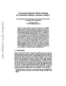
for greatest ones). For finite state spaces, there always is an index n such that Qn+1 = Qn holds. For infinite state spaces, the existence of such an index is not guaranteed, but we still have limi→∞ Qi = JσZ.ϕKK . Note that for sufficiently powerful base logics, the model checking problem for Lµ is undecidable. For the example shown in Figure 2, the fixpoint is reached after two iterations. In contrast, the fixpoint iteration does not terminate for the example shown in Figure 3.
According to the following definition, we denote the set of states that satisfy a formula ϕ ∈ Lµ by JϕKK .
2.3. Local Model Checking
Definition 4 (Semantics of the µ-Calculus) Let α ∈ L be a formula and K = (S, I, R) a Kripke structure, then the semantics of Lµ is defined as follows:
In contrast to global model checking, local model checking [9, 10, 18, 38, 39] aims at directly answering the question whether I ⊆ JϕKK holds. For that purpose, proof goals of the form Φ ⊢ ϕ are considered where Φ is a set of states and ϕ is a Lµ –formula. The meaning of a goal Φ ⊢ ϕ is that Φ ⊆ JϕKK has to be proved. In the following, we use formulas Φ ∈ L over the free variables x = (x1 , . . . , xn ) as symbolic representations of state sets. Proofs of such goals are obtained by syntax-directed decomposition into subgoals using the rules shown in Figure 1. The propositions above and below a line are equivalent for all rules.
JαKK :≡ JαK ∩ S JZKK :≡ {s ∈ S | s(Z)} Jϕ ∧ ψKK :≡ JϕKK ∩ JψKK Jϕ ∨ ψKK :≡ JϕKK ∪ JψKK J♦ϕKK :≡ preR J�ϕKK :≡ preR ∃ (JϕKK ) ∀ (JϕKK ) ← − ← − R J ♦ ϕKK :≡ sucR J � ϕKK :≡ suc∀ (JϕKK ) ∃ (JϕKK ) JµZ.ϕKK is the least set Q where Q = JϕKKQ holds Z JνZ.ϕKK is the greatest set Q where Q = JϕKKQ holds Z
Q KZ
is the Kripke structure obtained from K by changing the states s of K such that s(Z) holds iff s ∈ Q holds. A Kripke structure K = (S, I, R) satisfies a formula ϕ (K |= ϕ) iff I ⊆ JϕKK holds.
(1)
Φ⊢ϕ∧ψ Φ⊢ϕ∧Φ⊢ψ
As an example for the translation of temporal logic formulas to the µ-calculus, consider the CTL formula EGϕ that can be expressed in the µ-calculus by the formula νZ.ϕ ∧ �Z. The CTL* formula AF(ϕ ∧ Xϕ) (that cannot be expressed in CTL) is translated to µZ.(ϕ ∨ �Z) ∧ (¬ϕ ∨ �(ϕ ∨ Z)) (see [29] for such translations).
(2)
Φ⊢ϕ∨ψ ∃Ψ1 , Ψ2 . Ψ1 ⊢ ϕ ∧ Ψ2 ⊢ ψ ∧ Φ ⊆ Ψ1 ∪ Ψ2
(3)
Φ ⊢ �ϕ sucR ∃ (Φ) ⊢ ϕ
2.2. Global Model Checking
(5)
(4)
Global model checking algorithms compute all states JϕKK of a Kripke structure K where a formula ϕ holds. For that purpose, the algorithms traverse the syntax tree of ϕ in a bottom-up manner and attach to each subformula the corresponding set of states of K where the subformula holds. According to Definition 4, the Boolean operations, i.e., conjunction and disjunction, are computed by intersection and union of the corresponding state sets, respectively. Modal formulas are evaluated by computing the predecessors and successors of a set of states (Definition 3). The satisfying states of a fixpoint formula JσZ.ϕKK are obtained by the iteration Qi+1 := JϕKKQi starting with Z Q0 := ∅ for least fixpoints and with Q0 := S for greatest fixpoints. In both cases, the sequence Q0 . . . Qi is monotonic (increasing for least fixpoints, and decreasing
(6)
Φ ⊢ ♦ϕ ∃Ψ. Ψ ⊢ ϕ ∧ Φ ⊆ preR ∃ (Ψ) ← − Φ ⊢ �ϕ preR ∃ (Φ) ⊢ ϕ ← − Φ ⊢ ♦ϕ ∃Ψ. Ψ ⊢ ϕ ∧ Φ ⊆ sucR ∃ (Ψ)
(7)
Φ⊢Z Φ ⊢ ∆(Z)
(8)
Φ ⊢ σZ.ϕ ′ Φ ⊢ [ϕ]Z Z
∆ := ∆ ∪ {(Z ′ , σZ.ϕ)}
(9)
Φ⊢ϕ Φ ⊆ JϕKK
ϕ∈L
(10)
Φ⊢ϕ ∃Ψ. Ψ ⊢ ϕ ∧ Φ ⊆ Ψ
Figure 1. Decomposition rules for LMC
168 Authorized licensed use limited to: Technische Universitat Kaiserslautern. Downloaded on March 12, 2009 at 07:22 from IEEE Xplore. Restrictions apply.
Rule (1) simply splits a conjunction into two subgoals. When considering rules (3) and (5) one might be surprised that the universal modal operators are reduced to computing the existential successor states. This is due to the fact that after rewriting the expanded formulas, the universal quantifiers turn into existential ones [35]. Rule (2) is explained as follows: If Φ ⊢ ϕ ∨ ψ holds, then the set of states encoded by Φ can be partitioned into the set of states Ψ1 that satisfy ϕ and the set of states Ψ2 that satisfy ψ. The application of this rule requires that the user guesses suitable sets Ψ1 , Ψ2 such that the goal Φ ⊢ ϕ ∨ ψ can be decomposed into provable subgoals. In a similar way, rules (4) and (6) that implement the semantics of existential modal operators, require to have a suitable set of states Ψ. Rules that reduce a proposition to an existentially quantified one are often called choice rules. Their application requires that the user provides suitable witnesses, so that the remaining proof succeeds. Rules (7) and (8) unwind fixpoint formulas. To this end, the procedure maintains a so-called definition list ∆ that consists of pairs (Z, σZ.ϕ) that associate a bound variable Z with the subformula where it is bound1 . Provided that (Z, σZ.ϕ) ∈ ∆ holds, we write ∆(Z) for the second component of this pair. To avoid infinite recursion, it has to be checked whether the regeneration of a fixpoint formula leads to a previously created vertex with the same query. In this case, the construction of the proof is successful for greatest fixpoints. For least fixpoint formulas, it has to be checked whether the corresponding path in the proof tree is well-founded [9, 10]. The reason for this is a deeply rooted property of the µ-calculus that intuitively states that least fixpoints are related to finite recursion, while greatest fixpoints allow infinite recursion. Rule (9) is applied for formulas of the base logic and terminates the decomposition process. Finally, rule (10) is used to strengthen a goal Φ ⊢ ϕ by finding an appropriate superset of Φ. Again, this rule requires user interaction to set up a suitable lemma Ψ ⊢ ϕ. Reconsider the example shown in Figure 2. For this example, the construction of the proof does not terminate since the loop test fails each time the fixpoint variable Z is encountered. In contrast, LMC succeeds for the example shown in Figure 3.
2.4. Bounded Model Checking Bounded model checking is usually based on translating LTL formulas to formulas of the base logic. However, this can be generalized to the µ-calculus as will be shown in the following. 1 It is assumed that every variable is bound only once and has no additional free occurrences. Moreover, the formulas are given in guarded normal form [29], i.e., every occurrence of a bound variable Z in σZ.ϕ is guarded by a modal operator.
K = (Z, I, R) I :≡ x = 0 R :≡ x′ = x + 1 ∧ x ≥ 0 ϕ :≡ νZ. x ≥ 0 ∧ �Z 0
1
...
2
Q0 = JtrueKK Q1 = Jx ≥ 0KK Q2 = Q1 x = 0 ⊢ νZ. x ≥ 0 ∧ �Z x = 0 ⊢ x ≥ 0 ∧ �Z x=0⊢x≥0
x = 0 ⊢ �Z x=1⊢Z .. .
Figure 2. Example for GMC and LMC Definition 5 (Fixpoint Approximation) Given a fixpoint formula σZ.ϕ, its n-th approximation apxn (σZ.ϕ) is recursively defined as follows where [ϕ]ψ Z is the formula obtained by replacing all occurrences of Z with ψ: apx0 (µZ.ϕ) := false apx0 (νZ.ϕ) := true
apx (µZ.ϕ)
apxn+1 (µZ.ϕ) := [ϕ]Z n apx (νZ.ϕ) apxn+1 (νZ.ϕ) := [ϕ]Z n
Since by definition K |= ϕ iff I ⊆ JϕKK holds, and every sequence of fixpoint approximations is increasing for least fixpoints and decreasing for greatest fixpoints, the following implications hold for all i > 0: I ⊆ Japxi (µZ.ϕ)KK ⇒ K |= µZ.ϕ I 6⊆ Japxi (νZ.ϕ)KK ⇒ K 6|= νZ.ϕ Hence, estimating a bound i and checking the above conditions is sufficient to prove least fixpoints and to disprove greatest fixpoints. However, this is not sufficient to disprove least fixpoints and to prove greatest fixpoints. This limitation is the result of approximating the fixpoints: We can claim for the states in Japxi (µZ.ϕ)KK that the formula µZ.ϕ holds, but nothing can be said for all other states. Similarly, we know that the states that do not belong to Japxi (νZ.ϕ)KK fail to satisfy νZ.ϕ. However, there is no information for the states not included in this set.
169 Authorized licensed use limited to: Technische Universitat Kaiserslautern. Downloaded on March 12, 2009 at 07:22 from IEEE Xplore. Restrictions apply.
It is easily seen that for this encoding, the three-valued operators can be implemented by the two-valued ones, where x ⊔ y denotes the supremum of x and y:
K = (Z, I, R) I :≡ x ≥ 1 R :≡ x′ = x + 1 ϕ :≡ νZ. x 6= 0 ∧ �Z ...
-1
0
• • • • • • •
...
1
Q0 = JtrueKK Q1 = Jx 6= 0KK Q2 = Jx ≤ −2 ∨ x ≥ 1KK .. .
¬(ϕ1 , ϕ2 ) = (ϕ2 , ϕ1 ) (ϕ1 , ϕ2 ) ∧ (ψ1 , ψ2 ) = (ϕ1 ∧ ψ1 , ϕ2 ∨ ψ2 ) (ϕ1 , ϕ2 ) ∨ (ψ1 , ψ2 ) = (ϕ1 ∨ ψ1 , ϕ2 ∧ ψ2 ) (ϕ1 , ϕ2 ) → (ψ1 , ψ2 ) = (ϕ2 ∨ ψ1 , ϕ1 ∧ ψ2 ) ∃x.(ϕ1 , ϕ2 ) = (∃x.ϕ1 , ∀x.ϕ2 ) ∀x.(ϕ1 , ϕ2 ) = (∀x.ϕ1 , ∃x.ϕ2 ) (ϕ1 , ϕ2 ) ⊔ (ψ1 , ψ2 ) = (ϕ1 ∨ ψ1 , ϕ2 ∨ ψ2 )
In the following, three-valued formulas are represented by pairs of two-valued formulas in dual-rail encoding. The three-valued extension (ϕ, ¬ϕ) of a formula ϕ is denoted by ǫ(ϕ). Moreover, the equivalence of two functions is defined as (ϕ1 , ϕ2 ) ≡ (ψ1 , ψ2 ) = (ϕ1 ↔ ψ1 ) ∧ (ϕ2 ↔ ψ2 ).
x ≥ 1 ⊢ νZ. x 6= 0 ∧ �Z x ≥ 1 ⊢ x 6= 0 ∧ �Z
3. Three–Valued Bounded Model Checking x ≥ 1 ⊢ x 6= 0
x ≥ 1 ⊢ �Z
3.1. Bounded Global Model Checking
x≥2⊢Z
Figure 3. Example for GMC and LMC
2.5. Three–Valued Logic Three-valued logic [24] has been applied in many areas, e.g. for the analysis of asynchronous circuits [13], in compilers [28], for causality analysis [3, 25, 31, 32, 37], and for the analysis of cache behavior [1]. Given the values 0, 1, and ⊥, we define the partial order x ⊑ y as follows: ⊥ 0
1
The basic operators, i.e., negation, conjunction, and disjunction are defined by the following truth tables: x ⊥ 0 1
¬x ⊥ 1 0
∧ ⊥ 0 1
⊥ ⊥ 0 ⊥
0 0 0 0
1 ⊥ 0 1
∨ ⊥ 0 1
⊥ ⊥ ⊥ 1
0 ⊥ 0 1
1 1 1 1
To allow simple and elegant implementations, we use the following encoding which is known as dual-rail encoding in ternary simulation [30, 32]: x ǫ(x)
⊥ (0, 0)
0 (0, 1)
1 (1, 0)
The extension of global model checking to three-valued logic is straightforward: instead of considering two-valued characteristic functions, we represent a set Mλ by its threevalued function λ with the following meaning: 0 : if x 6∈ Mλ λ(x) := 1 : if x ∈ Mλ ⊥ : if neither x ∈ Mλ nor x 6∈ Mλ is known Using dual rail encoding, the characteristic functions are symbolically represented by pairs of (two-valued) formulas of the base logic L. For the characteristic function λ returned by an approximation of a least fixpoint, we have λ(x) ∈ {1, ⊥}, and analogously, for the characteristic function λ returned by an approximation of a greatest fixpoint computation, we have λ(x) ∈ {0, ⊥}. If we additionally check whether the obtained approximation already equals to the fixpoint, we can replace ⊥ in both cases by the missing boolean value. This can be done by checking whether apxi (σZ.ϕ) ↔ apxi+1 (σZ.ϕ) is valid2 . Figure 4 shows the algorithm for bounded global model checking (BGMC). According to Definitions 3 and 4, it syntactically unwinds a µ-calculus formula a bounded number of times to obtain a formula without fixpoint and modal operators. The algorithm returns a three-valued characteristic function that represents the states where the formula holds. The operators ∧, ∨, →, and the quantifiers are all threevalued operations that are implemented via dual-rail encoding as presented in Section 2.5. 2 As a consequence, the resulting formulas may contain alternating quantifiers which requires the use of SAT solvers for quantified logic.
170 Authorized licensed use limited to: Technische Universitat Kaiserslautern. Downloaded on March 12, 2009 at 07:22 from IEEE Xplore. Restrictions apply.
function BGMC(Φ ∈ L, ϕ ∈ Lµ , k ∈ N) : L × L return ∀x.ǫ(Φ) → Unwind(ϕ, k); end; function Unwind(ϕ ∈ Lµ , k ∈ N) : L × L case ϕ of L: return ǫ(ϕ); (∗ ϕ has free variables x ∗) ψ1 ∧ ψ2 : return Unwind(ψ1 , k) ∧ Unwind(ψ2 , k); ψ1 ∨ ψ2 : return Unwind(ψ1 , k) ∨ Unwind(ψ2 , k); ′ �ψ : return ∀x′ .ǫ(R) → [Unwind(ψ, k)]xx ; ′ ♦ψ : return ∃x′ .ǫ(R) ∧ [Unwind(ψ, k)]xx ; ← − �ψ : return [∀x.ǫ(R) → Unwind(ψ, k)]xx′ ; ← − ♦ψ : return [∃x.ǫ(R) ∧ Unwind(ψ, k)]xx′ ; σZ.ψ : if σ = µ then ϕ′ := 0; else ϕ′ := 1; end; for i := 0 to k − 1 do ′ ϕ′ := [ψ]ϕ Z ; end; ′ ϕ′′ := [ψ]ϕ Z ; ψ ′ := Unwind(ϕ′ , k); ψ ′′ := Unwind(ϕ′′ , k); Φ := ǫ(∀x.ψ ′ ≡ ψ ′′ ); if σ = µ then Ψ := ψ ′′ ∨ ¬(Φ ∨ ǫ(⊥)); else Ψ := ψ ′′ ∧ (Φ ∨ ǫ(⊥)); end; return Ψ; end; end; Figure 4. Bounded global model checking The fixpoint test is explained as follows: If ∀x.ψ ′ ≡ ψ ′′ is valid, the fixpoint is reached and we set Ψ := ψ ′′ ∨¬(ǫ(1)∨ ǫ(⊥)) for least fixpoints and Ψ := ψ ′′ ∧ (ǫ(1) ∨ ǫ(⊥)) for greatest fixpoints. In both cases, Ψ equals to ψ ′′ and thus, no information is lost. In contrast, if ∀x.ψ ′ ≡ ψ ′′ is not valid, the algorithm returns ψ ′′ ∨ ǫ(⊥) and ψ ′′ ∧ ǫ(⊥) for least and greatest fixpoints, respectively. This ensures that the result can only be 1 or ⊥ for least fixpoints and 0 or ⊥ for greatest fixpoints. Theorem 1 (Bounded Global Model Checking) Let x = (x1 , . . . , xn ) and x′ = (x′1 , . . . , x′n ) be vectors of variables with xi ∈ V and x′i ∈ V ′ . Moreover, let I ∈ L be a formula over the variables x and R ∈ L a formula over the variables x and x′ such that I represents the initial
states and R the transition relation of a Kripke structure K. Then, for all formulas ϕ ∈ Lµ and all k ∈ N with (ϕ1 , ϕ2 ) = BGMC(I, ϕ, k), we have: • if neither ϕ1 nor ϕ2 is true, then we know nothing about the truth of K |= ϕ • if ϕ1 is false and ϕ2 is true, then K 6|= ϕ • if ϕ1 is true and ϕ2 is false, then K |= ϕ As an example, reconsider Figure 2. For the formulas ϕ′ and ϕ′′ that are used for unwinding fixpoint formulas in Figure 4, we obtain: ϕ′ = x ≥ 0 ∧ �(x ≥ 0 ∧ 1) ϕ′′ = x ≥ 0 ∧ �(x ≥ 0 ∧ �(x ≥ 0 ∧ 1)) Eliminating the modal operators in ϕ′ and ϕ′′ yields: ψ ′ = ǫ(x ≥ 0) ∧ ∀x′ .ǫ(x′ = x + 1 ∧ x ≥ 0) → ǫ(x′ ≥ 0) ∧ ǫ(1) ψ ′′ = ǫ(x ≥ 0) ∧ ∀x′ .ǫ(x′ = x + 1 ∧ x ≥ 0) → ∀x.ǫ(x = x′ + 1 ∧ x′ ≥ 0) → ǫ(x ≥ 0) ∧ ǫ(1) Since ∀x.ψ ′ ↔ ψ ′′ holds, the fixpoint is reached and the algorithm returns ψ ′′ . Finally, it has to be checked whether ∀x.ǫ(x = 0) → ψ ′′ holds. Since this is the case, we can conclude that the specification is satisfied.
3.2. Bounded Local Model Checking The rules for local model checking presented in Section 2.3 are sufficient to prove every valid specification. Unfortunately, this often requires user interaction which is due to the disjunctive nature of the choice rules. Additionally, the user needs to know when to apply rule (10) which can be really challenging. Note that this rule allows LMC to switch to a different proof goal that requires to guess the right induction lemma. In practice, however, one is mainly interested in automatic proof procedures. For this reason, we restrict ourselves to the universal fragment of the µ-calculus that does not require the application of choice rules3 . Although this may seem to be a hard restriction, the remaining fragment is still powerful enough to automatically prove properties that cannot be proved by global model checking [35]. In addition, we use the following techniques to automate the decomposition process: • A goal Φ ⊢ ϕ ∨ ψ with ϕ ∈ L is reduced to the goal Φ ∧ ¬ϕ ⊢ ψ which is the least remaining requirement. • Checking repetition is not only successful if the same goal Φ ⊢ ϕ appears, but also if a goal Ψ ⊢ ϕ appears such that Ψ ⊆ Φ holds. This is used in the loop closure test before unwinding a fixpoint formula. 3 Existential properties can be proved by disproving the negated specification.
171 Authorized licensed use limited to: Technische Universitat Kaiserslautern. Downloaded on March 12, 2009 at 07:22 from IEEE Xplore. Restrictions apply.
• Least fixpoint formulas are always unwinded until the bound is reached. In this way, many least fixpoint formulas can be verified without having to check wellfoundedness of the proof tree.
listhL × Lµ i CallStack := []; function BLMC(Φ ∈ L, ϕ ∈ Lµ , k ∈ N) : L × L case ϕ of L: return ǫ(∀x. Φ → ϕ); ψ1 ∧ ψ2 : ϕ1 := BLMC(Φ, ψ1 , k); ϕ2 := BLMC(Φ, ψ2 , k); return (ϕ1 ∧ ϕ2 ); ψ1 ∨ ψ2 : if ψ1 ∈ L then return BLMC(Φ ∧ ¬ψ1 , ψ2 , k); end; if ψ2 ∈ L then return BLMC(Φ ∧ ¬ψ2 , ψ1 , k); end; return ǫ(⊥); �ψ : return BLMC([∃x.R ∧ Φ]xx′ , ψ, k); ← − ′ �ψ : return BLMC(∃x′ .R ∧ [Φ]xx , ψ, k); σZ.ψ : CallStack := cons((Φ, ϕ), CallStack); ϕ′ := BLMC(Φ, ψ, k − 1); CallStack := tail(CallStack); return ϕ′ ; Z: ψ := ∆(Z); if k > 0 then ϕ′ := BLMC(Φ, ψ, k); else ϕ′ := ǫ(⊥); end; if IsLeastFixpoint(ψ) then Ψ := ϕ′ ; else CS := CallStack; do (Φ′ , ψ ′ ) := head(CS); CS := tail(CS); while (ψ 6= ψ ′ ); Ψ := ǫ(∀x. Φ → Φ′ ) ∨ ϕ′ ; end; return Ψ; end; end;
Figure 5 shows the algorithm for BLMC. According to the rules of Figure 1, it recursively decomposes a µ-calculus formula into subformulas and returns a pair of formulas in dual-rail encoding. Formulas of the base logic can be directly reduced without further decomposition. The decomposition of conjunctions follows directly from rule (1) of Figure 1. Disjunctions require that at least one of the subformulas belongs to the base logic. If this is not the case, the algorithm returns the unknown value ⊥. Modal operators are decomposed4 according to rules (3) and (5) of Figure 1. The algorithm uses a call stack to keep track of the unwinded formulas. Every entry consists of a pair (Φ, ϕ) that represents a goal Φ ⊢ ϕ with ϕ = σZ.ψ. If such a goal is encountered, the algorithm pushes the pair (Φ, ϕ) on the call stack and continues with the goal Φ ⊢ ψ. After that, the top-level element is removed from the call stack. If the algorithm encounters a fixpoint variable Z, the corresponding formula is unwinded once more, provided that the bound has not yet been reached. Otherwise, the algorithm returns ⊥ which means that the truth of the specification cannot be decided. Additionally, a loop closure test is performed for greatest fixpoint formulas. For that purpose, the call stack is examined to determine the most recent entry with the same query. If the loop test does not succeed, the result of decomposing the expanded formula is returned. Theorem 2 (Bounded Local Model Checking) Let x = (x1 , . . . , xn ) and x′ = (x′1 , . . . , x′n ) be vectors of variables with xi ∈ V and x′i ∈ V ′ . Moreover, let I ∈ L be a formula over the variables x and R ∈ L a formula over the variables x and x′ such that I represents the initial states and R the transition relation of a Kripke structure K. Then, for all formulas ϕ ∈ Lµ and all k ∈ N with (ϕ1 , ϕ2 ) = BLMC(I, ϕ, k), we have: • if neither ϕ1 nor ϕ2 is true, then we know nothing about the truth of K |= ϕ • if ϕ1 is false and ϕ2 is true, then K 6|= ϕ • if ϕ1 is true and ϕ2 is false, then K |= ϕ Proof 1 Algorithm BLMC implements local model checking for the universal fragment of Lµ such that the number of unwinding steps of fixpoint operators is bounded by the constant k. Note that the construction of the proof tree does not require interactive rules. For this reason, a goal I ⊢ ϕ is true iff all leaf vertices of the proof tree are true. Due to the correctness of the proof tree construction of local model 4 We assume that the substitution operation renames variables so that no free occurrence of a variable is turned into a bound occurrence.
Figure 5. Bounded local model checking
checking, it follows that the validity of ϕ1 ∧ ¬ϕ2 implies that I ⊢ ϕ is true. The converse may not hold due to the restriction of the bound k. However, leaf vertices cannot be extended even if k is increased. Therefore, the non-validity of a leaf vertex implies that the root goal I ⊢ ϕ is false (note that there is no other way to construct a proof tree due to the absence of choice rules). Note that the result of a leaf vertex definitely returns a Boolean value.
172 Authorized licensed use limited to: Technische Universitat Kaiserslautern. Downloaded on March 12, 2009 at 07:22 from IEEE Xplore. Restrictions apply.
As an example, consider Figure 3 where we used the formulas I :≡ x ≥ 1 and R :≡ x′ = x + 1 to symbolically represent the initial states and the transition relation of Kripke structure K. The function call BLMC(I, ϕ, 1) for the specification ϕ :≡ νZ. x 6= 0 ∧ �Z returns a pair (ϕ1 , ϕ2 ) with: ϕ1 = (∀x.x ≥ 1 → x 6= 0) ∧ (∀x.(∃x′ .x = x′ + 1∧ x′ ≥ 1) → x ≥ 1) ϕ2 = ¬(∀x.x ≥ 1 → x 6= 0) As ϕ is valid, but ψ is not, it follows that K |= ϕ holds. Note that the existential quantifier in ϕ1 becomes a universal one when the formula is brought to prenex normal form. Thus, the resulting formulas are alternation-free in this case. Having reduced the model checking problem to a satisfiability problem of the base logic, we can employ the same backend tools to solve the final problem as for BGMC. Needless to say that these tools should first perform some precomputations. For example, checking the validity of a formula ϕ∧ψ can be done by checking whether ϕ and ψ are valid, provided that ϕ and ψ do not contain free variables. Moreover, conjunctions and disjunctions can be checked lazily, i.e., evaluating the first subformula may already yield the truth value, so that the second subformula needs not to be evaluated. Finally, real implementations can integrate the validity check with the reduction to the base logic. In this way, the leaves of a proof can be checked as soon as possible.
3.3. Combining BGMC and BLMC Due to the different nature of global and local model checking, it may be the case that one specification can be verified by BGMC, but not by BLMC (Figure 2) while another specification can be verified by BLMC, but not by BGMC (Figure 3). For the verification of infinite state systems, it is therefore desirable to combine both approaches to be able to check a larger class of specifications automatically. Even for finite state systems such a combination is beneficial, since one approach may yield a witness (counter-example) for a relatively small bound whereas the other requires a much larger bound, thus increasing the size of the resulting formulas. A straightforward combination of BGMC and BLMC is to separately call both procedures and to compute the supremum of the resulting formulas. More precisely, given a Kripke structure K = (S, I, R), a specification ϕ, and a bound k, then BGMC(I, ϕ, k) ⊔ BLMC(I, ϕ, k) is Boolean iff at least one of the procedures returns a Boolean value. Thus, we still get a definite answer if either of the procedures returns an unknown value. This simple combination suffices to check the specifications shown in Figure 2 and Figure 3.
For a more fine-grained combination, recall that global model checking algorithms return all states of a Kripke structure where a specification holds while local model checking algorithms take a set of states and determine whether the specification holds for this particular set. Thus, BLMC can call BGMC, but not vice versa. As a first step towards such a combination, modal formulas that do not contain fixpoint operators can always be evaluated using BGMC. This is accomplished by modifying the algorithm shown in Figure 5 as follows: L� : return BGMC(Φ, ϕ, k); With this extension, it is possible to check specifications that contain both existential and universal modal operators. As an example, consider the formula ϕ :≡ νZ.♦1 ∧ �Z that holds in a state iff all paths leaving this state are infinite (a Kripke structure K is reactive iff K |= ϕ holds). For a Kripke structure with I :≡ x ≥ 0 and R :≡ x′ = x + 1, this requires to prove the subgoal x ≥ 0 ⊢ ♦1. According the above extension, we obtain the formula ∀x.ǫ(x ≥ 0) → ∃x′ .ǫ(x′ = x + 1) ∧ ǫ(1) for this subgoal. As this formula is valid, the subgoal holds (the remaining proof goals also succeed). As the next step, we present a combination of BGMC and BLMC that allows us to check nested fixpoint formulas. ← − Consider the specification ϕ :≡ µY.(νZ.♦1 ∧ �Z) ∧ � Y shown in Figure 6. For the given set of initial states (which differs from the one in the above example), local model checking can verify the outer fixpoint formula, but not the inner one, and global model checking can verify the inner fixpoint formula, but not the outer one. As a consequence, neither BGMC nor BLMC can be used to verify this specification. However, the situation is different if we apply them on a fixpoint basis. For that purpose, the last line of the case statement in Figure 5 is modified as follows: return Ψ ⊔ BGMC(Φ, ψ, k); Again, we compute the supremum of both formulas to obtain maximum information. In this way, nested fixpoint formulas can be verified even if both methods fail for the whole formula.
4. Summary and Conclusion In its basic form, bounded model checking is only a semidecision procedure, i.e., it can neither be used to prove safety properties nor to disprove liveness properties. For finite state systems, this problem can be solved by additional techniques such as loop detection and completeness thresholds. However, these techniques increase the size of the resulting formulas and slow down the verification process. For infinite state systems, they may even fail completely.
173 Authorized licensed use limited to: Technische Universitat Kaiserslautern. Downloaded on March 12, 2009 at 07:22 from IEEE Xplore. Restrictions apply.
K = (Z, I, R) I :≡ x = c R :≡ x′ = x + 1 ∧ x ≥ 0 ← − ϕ :≡ µY.(νZ.♦1 ∧ �Z) ∧ � Y 0
1
2
References
...
← − x = c ⊢ µY.(νZ.♦1 ∧ �Z) ∧ � Y ← − x = c ⊢ (νZ.♦1 ∧ �Z) ∧ � Y x = c ⊢ νZ.♦1 ∧ �Z
our approach. Another issue is the use of first-order logic as the base logic. Although first-order logic is only semidecidable, it can also be used for a reduction of model checking problems to satisfiability problems.
← − x = c ⊢ �Y
BGMC(x = c, νZ.♦1 ∧ �Z, k) 0⊢Y
Figure 6. Example for combination of BGMC and BLMC
In this paper, we proposed the use of three-valued logic for bounded model checking in order to reason about positive, negative, and unavailable information. Moreover, we presented bounded variants of both global and local model checking to benefit from the different types of specifications that can be handled by these approaches. To the best of our knowledge, this is the first time where the ideas of local model checking are used for a reduction of model checking problems to corresponding satisfiability problems. In this way, we are not only able to disprove safety properties but in many cases also to prove them. Additionally, we showed how these procedures can be combined in the three-valued setting which is particularly important for infinite state systems. It is interesting to note that the presented combination is more than the sum of its parts. In other words, it allows us to check more specifications than can be checked with either approach alone. Even finite state systems can benefit from this synergetic effect: Although the size of the resulting formulas increase for a particular bound, this may be more than compensated by decreasing the actual bound. In the future, we plan to integrate the well-foundedness test for least fixpoint formulas in BLMC. Furthermore, it would be interesting to see whether recent developments in BMC such as interpolation [26] can be incorporated in
[1] M. Alt, C. Ferdinand, F. Martin, and R. Wilhelm. Cache behavior prediction by abstract interpretation. In Static Analysis Symposium (SAS), volume 1145 of LNCS, pages 52–66, Aachen, Germany, 1996. Springer. [2] C. Bartzis and T. Bultan. Automata-based representations for arithmetic constraints in automated verification. In J.M. Champarnaud and D. Maurel, editors, Conference on Implementation and Application of Automata (CIAA), volume 2608 of LNCS, pages 282–288, Tours, France, 2003. Springer. [3] G. Berry. The constructive semantics of pure Esterel. http://www-sop.inria.fr/esterel.org, July 1999. [4] A. Biere, A. Cimatti, E. Clarke, M. Fujita, and Y. Zhu. Symbolic model checking using SAT procedures instead of BDDs. In Design Automation Conference (DAC), pages 317–320, New Orleans, Louisiana, USA, 1999. ACM. [5] A. Biere, A. Cimatti, E. Clarke, O. Strichman, and Y. Zhu. Bounded model checking. Advances In Computers, 58, 2003. [6] A. Biere, A. Cimatti, E. Clarke, and Y. Zhu. Symbolic model checking without BDDs. In R. Cleaveland, editor, Conference on Tools and Algorithms for the Construction and Analysis of Systems (TACAS), volume 1579 of LNCS, pages 193–207, Amsterdam, The Netherlands, 1999. Springer. [7] B. Boigelot, A. Legay, and P. Wolper. Iterating transducers in the large. In W. Hunt and F. Somenzi, editors, Conference on Computer Aided Verification (CAV), volume 2725 of LNCS, pages 223–235, Boulder, Colorado, 2003. Springer. [8] A. Bouajjani, B. Jonsson, M. Nilsson, and T. Touili. Regular model checking. In E. Emerson and A. Sistla, editors, Conference on Computer Aided Verification (CAV), volume 1855 of LNCS, pages 403–418, Chicago, IL, USA, 2000. Springer. [9] J. Bradfield. Verifying Temporal Properties of Systems. Progress in Theoretical Computer Science. Birkhäuser, Boston, Basel, Berlin, 1992. [10] J. Bradfield and C. Stirling. Local model checking for infinite state spaces. In K. Larsen and A. Skou, editors, Workshop on Computer Aided Verification (CAV), July 1991. [11] G. Bruns and P. Godefroid. Model checking partial state spaces with 3-valued temporal logics. In N. Halbwachs and D. Peled, editors, Conference on Computer Aided Verification (CAV), volume 1633 of LNCS, pages 274–287, Trento, Italy, 1999. Springer. [12] R. Bryant. Graph-based algorithms for Boolean function manipulation. IEEE Transactions on Computers, C35(8):677–691, August 1986. [13] J. Brzozowski and C.-J. Seger. Asynchronous Circuits. Springer, 1995.
174 Authorized licensed use limited to: Technische Universitat Kaiserslautern. Downloaded on March 12, 2009 at 07:22 from IEEE Xplore. Restrictions apply.
[14] M. Chechik, B. Devereux, S. Easterbrook, and A. Gurfinkel. Multi-valued symbolic model-checking. ACM Transactions on Software Engineering and Methodology (TOSEM), 12(4):371–408, 2003. [15] E. Clarke, A. Biere, R. Raimi, and Y. Zhu. Bounded model checking using satisfiability solving. Formal Methods in System Design, 19(1):7–34, 2001. [16] E. Clarke, O. Grumberg, and D. Peled. Model Checking. MIT, London, England, 1999. [17] E. Clarke, D. Kroening, J. Ouaknine, and O. Strichman. Completeness and complexity of bounded model checking. In B. Steffen and G. Levi, editors, Verification, Model Checking, and Abstract Interpretation (VMCAI), volume 2937 of LNCS, pages 85–96, Venice, Italy, 2004. Springer. [18] R. Cleaveland. Tableaux-based model checking in the propositional µ-calculus. Acta Informatica, 27(8):725–747, 1989. [19] L. de Moura, H. Rueß, and M. Sorea. Bounded model checking and induction: From refutation to verification. In W. Hunt and F. Somenzi, editors, Conference on Computer Aided Verification (CAV), volume 2725 of LNCS, pages 14– 26, Boulder, Colorado, 2003. Springer. [20] D. Déharbe and A. Martins Moreira. Using induction and BDDs to model check invariants. In H. Li and D. Probst, editors, Conference on Correct Hardware Design and Verification Methods (CHARME), volume 105 of IFIP Conference Proceedings, pages 203–213, Montréal, Québec, Canada, 1997. Chapman & Hall. [21] N. Eén and N. Sörensson. Temporal induction by incremental SAT solving. Electronic Notes in Theoretical Computer Science (ENTCS), 89(4), 2003. [22] M. Fitting. Many-valued modal logics. Fundamenta Informaticae, 15(3-4):235–254, 1991. [23] M. Fitting. Many-valued modal logics II. Fundamenta Informaticae, 17(1-2):55–73, 1992. [24] S. Kleene. Introduction to Metamathematics. North Holland, 1952. [25] S. Malik. Analysis of cyclic combinational circuits. In Conference on Computer Aided Design (ICCAD), pages 618– 625, Santa Clara, California, November 1993. IEEE Computer Society. [26] K. McMillan. Interpolation and SAT-based model checking. In W. Hunt and F. Somenzi, editors, Conference on Computer Aided Verification (CAV), volume 2725 of LNCS, pages 1–13, Boulder, Colorado, 2003. Springer. [27] C. Meinel and T. Theobald. Algorithms and Data Structures in VLSI Design: OBDD – Foundations and Applications. Springer, 1998. [28] T. Reps, M. Sagiv, and R. Wilhelm. Static program analysis via 3-valued logic. In R. Alur and D. Peled, editors, Conference on Computer Aided Verification (CAV), volume 3114 of LNCS, pages 15–30, Boston, MA, USA, 2004. Springer. [29] K. Schneider. Verification of Reactive Systems – Formal Methods and Algorithms. Texts in Theoretical Computer Science (EATCS Series). Springer, 2003. [30] K. Schneider, J. Brandt, and T. Schuele. Causality analysis of synchronous programs with delayed actions. In Conference on Compilers, Architecture, and Synthesis of Embedded Systems (CASES), pages 179–189, Washington D.C., USA, September 2004. ACM.
[31] K. Schneider, J. Brandt, T. Schuele, and T. Tuerk. Improving constructiveness in code generators. In Synchronous Languages, Applications, and Programming (SLAP), Edinburgh, Scotland, UK, 2005. [32] K. Schneider, J. Brandt, T. Schuele, and T. Tuerk. Maximal causality analysis. In Conference on Application of Concurrency to System Design (ACSD), St. Malo, France, June 2005. IEEE Computer Society. [33] K. Schneider, R. Kumar, and T. Kropf. Alternative proof procedures for finite-state machines in higher-order logic. In J. Joyce and C.-J. Seger, editors, Higher Order Logic Theorem Proving and its Applications (TPHOL), volume 780 of LNCS, pages 213–226, Vancouver, Canada, 1993. Springer. [34] T. Schuele and K. Schneider. Bounded model checking of infinite state systems: Exploiting the automata hierarchy. In Formal Methods and Models for Codesign (MEMOCODE), pages 17–26, San Diego, CA, June 2004. IEEE. [35] T. Schuele and K. Schneider. Global vs. local model checking: A comparison of verification techniques for infinite state systems. In International Conference on Software Engineering and Formal Methods (SEFM), pages 67–76, Beijing, China, September 2004. IEEE. [36] M. Sheeran, S. Singh, and G. Stålmarck. Checking safety properties using induction and a SAT-solver. In W. Hunt and S. Johnson, editors, Conference on Formal Methods in Computer Aided Design (FMCAD), volume 1954 of LNCS, pages 108–125, Austin, Texas, USA, 2000. Springer. [37] T. Shiple. Formal Analysis of Synchronous Circuits. PhD thesis, University of California at Berkeley, 1996. [38] C. Stirling and D. Walker. Local model checking in the modal µ-calculus. In J. Diaz and F. Orejas, editors, Theory and Practice of Software Development (TAPSOFT), volume 351 of LNCS, pages 369–383. Springer, March 1989. [39] C. Stirling and D. Walker. Local model checking in the modal µ-calculus. Theoretical Computer Science, 89(1):161–177, 1991.
175 Authorized licensed use limited to: Technische Universitat Kaiserslautern. Downloaded on March 12, 2009 at 07:22 from IEEE Xplore. Restrictions apply.