This problem remains open: the BMC tools analyze an under- approximation of a program ... going to be refined and the algorithm goes to the next iteration. Our approach is ... analysis to guarantee a practical solution. Unlike in our ..... Classical BMC can prove the assertion up to some fixed recursion depth, but the result ...
Towards Completeness in Bounded Model Checking through Automatic Recursion Depth Detection Grigory Fedyukovich and Natasha Sharygina Faculty of Informatics, University of Lugano Via Guiseppe Buffi 13, CH-6904 Lugano, Switzerland
Abstract The presence of recursive function calls is a well-known bottleneck in software model checking as they might cause infinite loops and make verification infeasible. This paper proposes a new technique for sound and complete Bounded Model Checking based on detecting depths for all recursive function calls in a program. The algorithm of detection of recursion depth uses over-approximations of function calls. It proceeds in an iterative manner by refining the function over-approximations until the recursion depth is detected or it becomes clear that the recursion depth detection is infeasible. We prove that if the algorithm terminates then it guarantees to detect a recursion depth required for complete program verification. The key advantage of the proposed algorithm is that it is suitable for generation and/or substitution of function summaries by means of Craig Interpolation helpful to speed up consequent verification runs. We implemented the algorithm for automatic detection of recursion depth on the top of our SAT-based model checker FunFrog and demonstrate its benefits on a number of recursive C programs.
1
Introduction
Model checking plays an important role in both proving program correctness and finding bugs. It provides a powerful fully automated engine which is able to search for an assertion violation among all possible combinations of the input values. These advantages are however hindered by the high complexity of analysis, known as the state-space explosion phenomenon. To combat this problem, many effective state-space reduction solutions have been developed to allow model checking to scale to verification of complex systems. The most successful solutions are symbolic model checking among which are Bounded Model Checking (BMC) [2], and abstraction-based approaches such as predicate abstraction [8], interpolation-based reasoning [11], and function summarization [12,13,1,19]. BMC has been shown to be particularly successful in safety analysis of software. The state-of-the-art BMC-based tools such as CBMC [3], LLBMC [14], VeriSoft [9], FunFrog [18], just to name a few, have been successfully applied to verification of industrial-size programs. The well-known limitation of BMC is that it is aimed at searching for errors in a program within the given number
(bound) of loop iterations and recursion depth. For this reason, BMC is suitable only for program falsification, while for complete verification it requires finding a sufficient bound. This problem remains open: the BMC tools analyze an underapproximation of a program using some particular bound, defined a priori by the user or set by the tool to some constant, and check the program only up to this bound. There exists a number of (direct and indirect) solutions for the automatic loop bound detection (i.e., constant propagation, k-induction, loop summarization, etc). However, dealing with recursive function calls is more complicated and more expensive in practice. This paper proposes an approach for the automatic recursion depth detection in BMC and shows its applicability in practice. In particular, we present a BMC algorithm enhanced with automated construction of the sufficient unwinding1 . The algorithm iteratively explores the program calltree and over-approximates recursive function calls while treating precisely the other ones. The entire abstraction of the calltree is then checked onthe-fly with respect to a given assertion. If the assertion holds in the current level of abstraction then the corresponding unwinding is sufficient to guarantee complete verification (and the length of the longest unwinding chain constitutes the recursion depth). Otherwise, the algorithm identifies which over-approximated function calls are responsible for the assertion violation. These function calls are going to be refined and the algorithm goes to the next iteration. Our approach is developed to reach efficiency in BMC. At each iteration, it refines only a minimal set of over-approximated function calls, i.e., only those responsible for spuriousness of the error on the previous iteration. Clearly, the algorithm is not guaranteed to terminate when there are unbounded sequences of recursive calls in the program. But if for every possible value of input parameters, every recursive function in the real program is called a fixed number of times, the algorithm automatically detects this number and terminates. We further demonstrate how our algorithm can be made practical by extending our earlier work on construction and reusing of interpolation-based function summaries in BMC [19] for checking different assertions. In the current work, aside from checking user-provided assertions, we use a heuristic called assertion decomposition to artificially implant helper-assertions into the recursive program. These assertions are then checked incrementally to generate function summaries that will be reused to speed up verification of the user-provided assertions. We implemented the approach on the top of FunFrog BMC, previously restricted to work only for a user-supplied recursion depth. We evaluated it on a range of academic and industrial recursive programs requiring bitwise and nonlinear reasoning. Our experimentation confirmed that the summarization-based recursion depth detection in many cases makes BMC complete and dramatically improves its performance compare to the classical BMC approach (e.g., CBMC). Algorithmically, the closest body of work is the Corral [10] tool (see related work section for detailed comparison). It is a solver for a restricted version of the 1 The algorithm relies on the output of a loop bound detection routine (e.g., conversion loops to recursion) done by an external tool or set by the user.
reachability-modulo-theories problem, and it also uses summaries in its bounded analysis to guarantee a practical solution. Unlike in our approach, in the Corral, 1) the depth of recursion is bounded by a user-supplied recursion depth and 2) an external tool [7] is used to generate function summaries which in general may not be helpful to verify the given assertion. Our approach is able to generate relevant function summaries by itself. Moreover, it forces summaries to be bitprecise and highly related to the given assertion. It makes our algorithm converge more effectively and faster. The rest of the paper is structured as follows. Sect. 2 defines the notation and presents background on BMC, function summarization and refinement. Sect. 3 presents the BMC algorithm with automatic detection of recursion depth, proves its correctness and demonstrates its application to function summarization-based model checking. Sect. 4 discusses different experimentation scenarios of the approach including the assertion decomposition heuristic. Sect. 5 provides a comparison with the related work and Sect. 6 concludes the paper.
2
Preliminaries and Previous Work
We first define basic constructs required to present the new algorithm. In particular, we explicitly define recursion, function summaries and basic BMC steps. 2.1
Programs, function calls, recursion depth
Definition 1 (cf. [19]). An unwound program for a depth ν is a tuple Pν = (Fˆν , fˆmain , child), such that Fˆν is a finite set of function calls, unwound up to the depth ν, fˆmain ∈ Fˆν is a program entry point and child ⊆ Fˆν × Fˆν relates each function call fˆ to all function calls invoked directly from it. There is a fixed set F to represent functions declared in the program and a possibly unbounded set Fˆ to represent function calls. A call fˆ ∈ Fˆ corresponds to a call of a target function, determined by a mapping target : Fˆ → F . A subset Fˆν ⊆ Fˆ is introduced to help handling recursion. There is exactly one call of function fmain , but there may be several calls of the other functions. For simplicity, later we will use primes (i.e., fˆ0 , fˆ00 ,..) and indexes (i.e., fˆ1 , fˆ2 ,..) to differentiate the calls of the same function f ∈ F in the unwound program. The set of function calls Fˆ together with the relation child can be represented by a corresponding calltree with the root fˆmain . We also use relation subtree ⊆ Fˆ ×Fˆ , a reflexive transitive closure of child. Now we can define recursive functions using this notation. Definition 2. A function f is recursive if for every call fˆi , there is another call fˆi0 in its subtree, and target(fˆi ) = target(fˆi0 ) = f . According to Def. 2, the calltree of a program with recursive functions is infinite. As detailized later in this section, for classical BMC it has to be bounded. A recursive function f is unwound ν times if there is a sequence of function calls
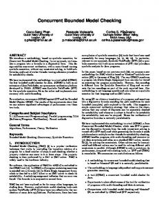
(later called an unwinding chain) fˆ0 , fˆ1 ,.. fˆν , where 1 ≤ i ≤ ν, target(fˆi ) = f , and each fˆi+1 is in the subtree of fˆi . The set of function calls Fˆν and the relation child define a finite corresponding calltree. If there are no recursive function calls in the program Pν = (Fˆ , fˆmain , child) then Fˆν ≡ Fˆ for any ν. BMC is aimed at checking assertions in a program within the given bound of loop iterations and recursion depth. If the unwinding number ν is provided a priori, BMC unrolls the loops and recursion up to ν, encodes the program symbolically and delegates the checking to a SAT solver. If the number is not provided a priori, BMC may go into an infinite loop and not terminate. Typically in the absence of the number or when the number is set too high, a predefined timeout is used to cope with this problem. BMC encodes the program into the Static Single Assignment (SSA) form, where each variable is assigned at most once. The SSA form is then conjoined with the negation of the assertion condition and converted into a logical formula, called a BMC formula. The BMC formula is checked for satisfiability, and every its satisfying assignment identifies an error trace. Otherwise, the program is safe up to ν. Notably, this unwinding number may not be sufficient for complete verification. A program can be proven safe for ν, but buggy for ν + 1. Fig. 1 illustrates BMC encoding for a simple C program (Fig. 1a) with a recursive function f. For this example, the recursion depth ν = 5 guarantees complete verification.2 In this setting, it is assumed that this recursion depth is
y0 = 1; x0 = nondet(); int f(int a) { if (x0 > 5) { if (a < 10) a0 = x0; return f (a + 1); // f (unwind 1) return a - 10; if (a0 < 10) } // f (unwind 2) ... void main() { // end f (unwind 2) ret0 = ...; int y = 1; int x = nondet(); else ret1 = a0 - 10; if (x > 5) ret2 = phi(ret0, ret1); y = f(x); // end f (unwind 1) y1 = ret2; assert(y >= 0); } } y2 = phi(y0, y1); assert(y2 >= 0); (a) C code (b) SSA form
y0 = 1 ∧ x0 = nondet 0 ∧ a0 = x0 ∧ ret 0 = ... ∧ ... ∧ ret 1 = a0 − 10 ∧ (x0 > 5 ∧ a0 < 10 ⇒ ret 2 = ret 0 ) ∧ (x0 > 5 ∧ a0 ≥ 10 ⇒ ret 2 = ret 1 ) ∧ y1 = ret 2 ∧ (x0 > 5 ⇒ y2 = y1 ) ∧ (x0 ≤ 5 ⇒ y2 = y0 ) ∧ y2 < 0
Figure 1: BMC formula generation 2
see more details on termination in Sect. 3.1
(c) BMC formula
given a priori. During unwinding (Fig. 1b), a call of function f is substituted by its body. There will be five such nested substitutions, and the sixth call is simply skipped in the example. The encoded BMC formula is shown on Fig. 1c. Classical BMC algorithms use a monolithic BMC formula, as described in details in [3]. For specialized BMC algorithms (such as in our earlier work on function summarization [19] and upgrade checking [6], and the new algorithm for automatic detection of recursion depth) it is convenient to use a so called Partitioned BMC formula, which is going to be presented in Sect. 2.2. 2.2
PBMC encoding
Definition 3 (cf. [19]). Let Fˆν be an unwound calltree, π encodes an assertion, φfˆ symbolically represent the body of a function f , a target of the call fˆ. Then V a partitioned BMC (PBMC) formula is constructed as ¬π ∧ fˆ∈Fˆν φfˆ. Fig. 2 demonstrates creation of a PBMC formula for the example from Fig. 1a. In the example program, unwound 5 times, the partitions for function calls f1 ,f2 ,..f5 and main are generated separately. They are bound together using a special boolean variable callstart fˆ for every function call fˆ. Intuitively, callstart fˆ is equal to true iff the corresponding function call fˆ is reached. Note that the assertion π is not encoded inside φfˆmain , as in classical BMC, but separated from the rest of the formula, such that it helps interpolation.3 Formula φfˆ1 that encodes the function call f1 aims to symbolically represent the function output argument ret 0 by means of the function input argument a0 , symbolically evaluated in φfˆmain . At the same time, φfˆ1 relies on the value of ret 3 defined in φfˆ2 by means of a1 . Similar reasoning is applied to create each of the following partitions: φfˆ2 ,.. φfˆ5 .
(a0 < 10 ⇔ callstart fˆ2 ) ∧ y0 = 1 ∧
a1 = a0 + 1 ∧
x0 = nondet 0 ∧
ret 1 = ret 3 ∧
a0 = x0 ∧
ret 2 = a0 − 10 ∧
x0 > 5 ⇔ callstart fˆ1 ∧
(callstart fˆ1 ∧ a0 < 10 ⇒ ret 0 = ret 1 ) ∧
y1 = ret 0 ∧
(callstart fˆ1 ∧ a0 ≥ 10 ⇒
(x0 > 5 ⇒ y2 = y1 ) ∧ (x0 ≤ 5 ⇒ y2 = y0 ) (a) formula φfˆmain
y2 ≥ 0 ⇔ π (b) definition of π
ret 0 = ret 2 ) (c) formula φfˆ1
Figure 2: PBMC formula generation 3
see more details on interpolation in Sect. 2.3
2.3
Craig Interpolation and Function Summarization
Definition 4 (cf. [4]). Given formulas A and B, such that A ∧ B is unsatisfiable. Craig Interpolant of A and B is a formula I such that A → I, I ∧ B is unsatisfiable and I is defined over the common alphabet to A and B. For mutually unsatisfiable formulas A and B, an interpolant always exists [4]. For quantifier free propositional logic, an interpolant can be constructed from a proof of unsatisfiability [16]. Interpolation is used to generate function summaries to speed up incremental verification (see our earlier work [19,18]). Definition 5 (cf. [19]). Function summary is an over-approximation of the function behavior defined as a relation over its input and output variables. A summary contains all behaviors of the function and (due to its overapproximating nature) possibly more. The infeasible behaviors (detected during analysis of abstract models) have to be refined by means of the automated procedure, as will be described in Sect. 2.4. If the program is safe with respect to an assertion π, then the PBMC formula representing the program is unsatisfiable. The interpolation procedure is applied repeatedly for each function call fˆ. It splits the PBMC formula into two parts, φsubtree and φenv (1). The former encodes the subtree of fˆ. The latter corresponds fˆ fˆ to the rest of the encoded program including a negation of assertion π. φsubtree ≡ fˆ
^
φgˆ
φenv ≡ ¬π ∧ fˆ
g ˆ∈Fˆ :subtree(fˆ,ˆ g)
^
φhˆ
(1)
ˆ Fˆ :¬subtree(fˆ,h) ˆ h∈
Since φsubtree ∧ φenv is unsatisfiable, the proof of unsatisfiability can be used fˆ fˆ to extract an interpolant Ifˆ for φsubtree and φenv . Such formula Ifˆ is then considfˆ fˆ ˆ ered as a summary for the function call f . While verifying another assertion π 0 , the entire part φsubtree of the PBMC formula will be replaced by the summary fˆ formula Ifˆ. 2.4
Counter-Example Guided Refinement
Definition 6 (cf. [19]). A substitution scenario for function calls is a function Ω : Fˆ → {inline, sum, havoc}. For each function call, a substitution scenario determines a level of approximation as one of the following three options: inline when it processes the whole function body; sum when it substitutes the call by an existing summary, and havoc when it treats the call as a nondeterministic function. Since havoc abstracts away the function call, it is equivalent to using a summary true. In the incremental abstraction-driven analyses [19,6], substitution scenarios are defined recurrently. Algorithms start with the least accurate initial scenario
Ω0 , and iteratively refine it. In (2) and (3), we adapt the definitions from [19] to the recursive case. there exists a summary of fˆ fˆ is not recursive or ν is not exceeded fˆ is recursive and ν is exceeded
(2)
inline, if Ωi (fˆ) 6= inline and callstart fˆ = true Ωi (fˆ), otherwise
(3)
sum, if Ω0 (fˆ) = inline, if havoc, if ( Ωi+1 (fˆ) =
When a substitution scenario Ωi leads to a satisfiable PBMC formula (i.e., there exists an error trace �), an analysis of � is required to shows that the error is either real or spurious. By construction of the PBMC formula, for each function call fˆ, a variable callstart fˆ is evaluated to true iff fˆ appears along �. Consequently, each fˆ might be responsible for spuriousness of � if fˆ was not precisely encoded and callstart fˆ = true. If there is no function call, satisfying the above mentioned conditions, � is real and must be reported to the user.
3
Bounded Model Checking with Automated Detection of Recursion Depth
This section presents an iterative abstraction-refinement algorithm for BMC with automated detection of recursion depth. We first present a basic algorithm, where all function calls are treated nondeterministically (Sect. 3.1). Then we strengthen this algorithm to support generation and use of interpolation-based function summaries (Sect. 3.2). 3.1
Basic Algorithm
An overview of the algorithm is depicted in Alg. 1. The algorithm starts with a preset recursion depth ν 4 and iterates until it detects the actual recursion depth, needed for complete proof of the program correctness, or a predefined timeout is reached. Notably, at each iteration of the algorithm, ν gets updated and is equal to the length of the longest unwinding chain of recursive function calls. In the end of the algorithm, all recursive calls are unwound exactly same number of times as they would be called during the execution of the program. The details of the computation are given below. First, the algorithm aims to construct a PBMC formula φ using the sets Fˆν and T. Every function call fˆ ∈ Fˆν is encoded precisely, every function call gˆ ∈ T is treated nondeterministically. In particular, bodies of function calls from set Fˆν are encoded into the SSA forms 4 The algorithm can be initialized with any number value as demonstrated in our experiments.
Algorithm 1: BMC with automatic detection of recursion depth
1 2 3
Input: Initial recursion depth: ν; Program unwound ν times: Pν = (Fˆν , fˆmain , child); Assertion to be checked: π; TimeOut Output: Verification result: {SAFE, BUG, TimeOut}; Detected recursion depth: ν; Error trace: � Data: PBMC formula: φ; temporary set of function calls to be refined: T while (¬TimeOut) do T ← {ˆ g∈ / Fˆν | child(fˆ, gˆ), fˆ ∈ Fˆν }; // get refinement candidates V V φ ← ¬π ∧ fˆ∈Fˆ CreateFormula(fˆ) ∧ gˆ∈T Nondet(ˆ g ); ν
4 5 6 7 8 9 10 11 12 13 14 15 16
result, sat_assignment ← Solve(φ); // run SAT solver if (result = UNSAT) then return SAFE, ν; else � ← extract_CE(sat_assignment); // extract error trace T ← T ∩ extract_calls(�); // filter out calls which do not affect SAT if (T = ∅) then return BUG, ν, �; else Fˆν ← Fˆν ∪ T; // unwind the calltree on demand ν ← max_chain_length(Fˆν ); // update the depth end return TimeOut
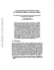
(i.e., method CreateFormula) and put together into separate partitions (one partition per each function call) of φ (line 3). At the same time, all function calls from T are replaced by true (i.e., method Nondet). In total, φ encodes a program abstraction containing precise and over-approximated parts, conjoined by negation of an assertion π (line 3). Fig. 3a demonstrates a calltree of a program with a single recursive function called twice at the first iteration of the algorithm. ˆ 1 , fˆ1 , fˆ2 } (grey nodes) are encoded precisely, In the example, Fˆν = {fˆmain , gˆ1 , h 0 ˆ ˆ and T = {f3 , f2 } (white nodes) are treated nondeterministically. After the PBMC formula φ is constructed, the algorithm passes it to a SAT solver. If φ is satisfiable, and the SAT solver returns a satisfying assignment (line 7), function calls from T are considered as candidate calls to be refined. To refine, the satisfying assignment is used to restrict T on the calls, appeared along the error trace � (i.e., in the satisfying assignment) (line 9). In the next iteration of the algorithm, the calls from T are encoded precisely in the updated PBMC formula. Technically, the algorithm extends Fˆν by adding function calls from T (line 13), as shown, for example, on Fig. 3b. There, fˆ20 appears along � and therefore it has to be refined; fˆ3 does not appear in �, so it will be encoded nondeterministically. If T = ∅ then no nondeterministically treated recursive calls were found along the error trace, so the real bug is found (line 11), and the algorithm terminates. If the SAT solver proves unsatisfiability of φ then the program abstraction, and consequently the program itself, are safe (line 6). This case is represented on Fig. 3c. The final recursion depth ν is detected, and the algorithm terminates. Theorem 1. Given the program P and an assertion π, if Alg. 1 terminates with
(a) gˆ1
fˆ1
fˆ2
fˆ0 ? 2
?
(b)
fˆmain
fˆ3
ˆ1 h
(c)
fˆmain
gˆ1 fˆ2 fˆ3
fˆ1
!
ˆ1 h
fˆ20 ?
fˆ30
fˆmain fˆ1
gˆ1 fˆ2 fˆ3 !
0
ˆ1 h
fˆ20
! !
2
fˆ30
!
1
3
fˆ⌫ fˆ⌫
1
⌫
1
⌫
Figure 3:
Illustration of the individual steps of the Alg. 1 on the example with a single recursive function f , called twice. ˆ 1 , fˆ1 , fˆ2 } (grey nodes) are encoded precisely, T = {fˆ3 , fˆ0 } (white a) First iteration: Fˆν = {fˆmain , g ˆ1 , h 2 "?" nodes) are treated nondeterministically; the initial recursion depth is equal to 1. b) Second iteration: solver returns SAT (corresponding to error trace � = {fˆmain , fˆ1 , fˆ20 }), set T is updated to contain only one function call ({fˆ20 } (black "!" nodes)). All calls from T are added to current Fˆν . The current recursion depth is incremented, and equal to 2. c) Final iteration: solver returns UNSAT or T = ∅, the detected recursion depth is equal to ν − 1.
an answer SAFE (BUG) then π holds (does not hold) for P . Proof (Proof sketch). The proof is divided into two parts, for SAFE (line 6) and BUG (line 11) outputs of the algorithm (and respectively, the PBMC formula φ proven UNSAT or SAT). Case SAFE. In this case φ is unsatisfiable. The formula φ represents some abstraction of P which contains precise and over-approximated components (as described in section 3.1). Since every abstracted formula can be strengthened and turned into the corresponding precise encoding, and since unsatisfiability of a weaker formula implies unsatisfiability of a stronger formula, then the PBMC formula φinline encoding P without abstraction is also unsatisfiable, i.e., π holds. Case BUG. In this case, φ is satisfiable, and the satisfying assignment represents an error trace. At the same time, the algorithm did not detect any nondeterministically treated recursive function calls along the error trace (line 10). It means that π is indeed violated within the current recursion depth. t u
Note on Termination. The algorithm is guaranteed to terminate within a given timeout when it finds an error or proves that the assertion holds. Similar to classical BMC, Alg. 1 terminates if the recursion depth is sufficient to disprove the assertion. Classical BMC can prove the assertion up to some fixed recursion depth, but the result might be incomplete if the recursion depth is insufficient. In contrast, by Theorem 1, if our algorithm does not yield a timeout, it guarantees that the detected recursion depth is complete to prove (disprove) the assertion. The other benefit of our algorithm is that it does not require the recursion depth to be given a priori, but instead it is detected automatically.
Algorithm 2: Summarization in BMC with Automatic Detection of Recursion Depth
1 2 3 4 5
Input: Initial recursion depth ν; Program unwound ν times: Pν = (Fˆν , fˆmain , child); Assertion to be checked: π; Set of summaries: summaries; TimeOut Output: Verification result: {SAFE, BUG, TimeOut}; Error trace: � Data: PBMC formula: φ; set of function calls: T; substitution scenario: Ω φ ← ¬π; // initialize φ T ← Fˆν ∪ {ˆ g∈ / Fˆν | child(fˆ, gˆ), fˆ ∈ Fˆν }; // unwind the calltree initially Ω ← init; // use (2) from Sect. 2.4 to create initial scenario while (¬TimeOut) do V V φ ← φ ∧ fˆ∈T:Ω(fˆ)=inline CreateFormula(fˆ) ∧ gˆ∈T:Ω(ˆ ApplySummaries(ˆ g) ∧ g )=sum V ˆ Nondet(h); // add partitions to φ (inline, summarize, havoc ) ˆ ˆ h∈T:Ω( h)=havoc
6 7 8 9 10 11 12 13 14 15 16 17 18
19 20
result, proof , sat_assignment ←Solve(φ); if (result = UNSAT) then foreach (fˆ ∈ T) do // split φ ≡ φsubtree ∧ φenv as in Sect. 2.3 fˆ fˆ ˆ ˆ summaries(f ) ← Interpolate(proof , f ); end return SAFE; else � ← extract_CE(sat_assignment); if (∅ = {fˆ ∈ extract_calls(�) | Ω(fˆ) 6= inline}) then return BUG, �; else Ω ← Refine(Ω, T, extract_calls(�)); // use (3) in Sect. 2.4 T ← T ∪ {ˆ g∈ / T | child(fˆ, gˆ), fˆ ∈ T, Ω(fˆ) = inline}; // // unwind the calltree on demand end return TimeOut
Based on our observations, termination of Alg. 1 depends on the termination of the recursive program it was applied to. For example, the program with one single recursive function from Fig. 1a terminates for any values of input data. The recursion termination condition, ¬(a < 10) defines the upper bound 10 for the value of a, and at the same time the function f monotonically increments the value of a. Hence, the recursive function f is called a fixed number of times and the program eventually terminates. Clearly, for complete analysis of this program it is enough to consider the maximum possible number of recursive function calls for every initial value of a which in this example is equal to 5. At the same time, it introduces an upper bound for the size of the constructed PBMC formula which is a sufficient condition to the SAT solver to terminate while solving it. 3.2
Optimizations and Applications of Alg. 1
Incremental Formula Construction and Refinement. Possible optimizations of Alg. 1 are 1) the incremental construction of the PBMC formula φ and 2) more efficient handling of a set of the refinement candidates, T. In the first optimization, φ is created in an incremental manner. At each iteration, φ is not recomputed from scratch, but gets conjoined with new partitions.
These partitions precisely encode the refined function calls from the set T. In this manner the PBMC formula is updated at the beginning of each iteration. In the second optimization, the set of refinement candidates T is merged with the whole set of unwound function calls Fˆν . Instead of handling those two sets, it is enough to handle one. To distinguish function calls which were present in T from the others present in Fˆν the substitution scenario Ω is used. Summarization. The proposed algorithm for recursion depth detection can be exploited for efficient incremental program verification (i.e., verification of the same program with respect to different assertions [19].5 In this setting, function summaries are computed by means of Craig Interpolation. Alg. 2 shows how the optimized Alg. 1 can be integrated with summarizationbased verification. Interpolating procedure (line 9), that employs the PBMC formula φ and its proof of unsatisfiability, is run after each assertion is proven. The use of summaries makes the verification more flexible. Instead of treating recursive function calls nondeterministically, the algorithm might apply existent summaries, thus making entire program abstraction more accurate. Moreover, the use of substitution scenario (line 5)enables summarization of any (not necessarily recursive) function calls.
4
Experimental Evaluation
We implemented the automatic Recursion Depth Detection (RDD) and Summarization-based RDD (SRDD) inside of the BMC tool FunFrog [18] and make its binary (FunFrog+(S)RDD) available6 . FunFrog supports interpolation-based function summarization for C programs and uses the SAT-solver PeRIPLO [17] for solving propositional formulas, proof reduction and interpolation. FunFrog follows CProver’s7 paradigm. In particular, it accepts a precompiled goto-binary, a representation of the C program in an intermediate goto-cc language, and runs the analysis on it. We evaluated the new algorithms on a set of various recursive C programs (taken from the SVCOMP’148 set (Ackermann X McCarthy, GCD, EvenOdd), obtained from industry9 (P2P_Joints X), crafted by USI students for evaluation of interpolation-based abstractions). We provide two verification scenarios to evaluate the algorithms. In the first one, FunFrog+RDD verifies a single assertion in each benchmark and detects the recursion depth. In the second one, FunFrog+SRDD incrementally verifies a set of assertions and reuses function summaries between its checks. In our experiments loop handling was done by means of CProver (see Sect. 5 for more details). 5 Recall that the analysis in [19] is restricted to programs, unwound fixed number of times (i.e., without recursion). 6 http://www.inf.usi.ch/phd/fedyukovich/funfrog_srdd.tar.gz 7 http://www.cprover.org 8 http://sv-comp.sosy-lab.org/2014/ 9 in scope of FP7-ICT-2009-5 — project PINCETTE 257647
benchmark name #R T Result In Array A 5 a SAFE 1 Array B 12 a SAFE 1 Array C 3 a SAFE 1 Ackermann A 2 b SAFE 1 Ackermann B 2 b BUG 1 Alternate A 2 c SAFE 1 Alternate B 2 c BUG 1 Multiply 10 a SAFE 1 InterleaveBitsRec 1 a SAFE 1 BitShiftRec A 1 a SAFE 1 BitShiftRec B 2 b SAFE 1 P2P_Joints A 1 a SAFE 1 P2P_Joints B 1 a BUG 1
FunFrog+RDD In≡1 1 < In < ν Time #It ν #Calls In Time #It 664.02 15 15 75 10 513.986 6 777.432 24 24 71 2 1781.92 23 1113.68 27 16 106 14 991.724 3 55.758 34 20 2169 7 3493.64 10 56.772 30 17 1942 7 3547.29 10 35.068 50 50 100 30 22.206 20 92.314 77 77 154 50 53.315 28 710.517 110 10 110 7 569.559 4 150.053 33 33 33 15 125.241 19 128.074 64 64 64 20 13.416 45 65.537 12 12 4285 3 65.399 10 1234.71 4 4 4 2 1195.31 3 1266.38 4 4 4 2 1222.11 3
In 15 24 16 20 17 50 77 10 33 64 12 4 4
In≡ ν Time #It 121.381 1 3600+ — 557.281 1 3600+ — 3600+ — 0.902 1 1.681 1 226.659 1 8.188 1 2.413 1 3600+ – 1092.26 1 1120.03 1
FunFrog
CBMC
Time 3600+ 3600+ 3600+ 3600+ 3600+ 3600+ 3600+ 3600+ 3600+ 3600+ 3600+ 3600+ 3600+
Time 3600+ 3600+ 3600+ 3600+ 3600+ 3600+ 3600+ 3600+ 3600+ 3600+ 3600+ 3600+ 3600+
Table 1: Verification statistics for various BMC tools with and without automated detection of recursion depth.
4.1
Evaluating RDD
Table 1 summarizes the verification statistics of a set of benchmarks with different types (T) of recursion (a - single recursion, b - multiple recursion, c indirect recursion). The number of recursive functions present in each benchmark is depicted in the column marked #R. Each benchmark was verified using CBMC, FunFrog10 without recursion depth detection and 3 different versions of FunFrog+RDD. The first configuration of FunFrog+RDD performs the algorithm with the initial recursion depth set to 1 (denoted as In ≡ 1 in the table), detects recursion depth (ν) and also reports the number of unwound recursive calls as #Calls. Then, in purpose of comparison, the second and the third configurations perform the same algorithm with the another values of the initial recursion depths (1 < In < ν and In ≡ ν respectively). For each experiment, we report total verification time (in seconds) and a number of iterations of FunFrog+RDD (#It). The verification results (SAFE/BUG) were identical for experiments with all configurations and we placed them in the table in the section describing the benchmarks. Notably, for all different types of recursion, the experiments with CBMC and pure FunFrog failed as they reached the timeout (3600+) of 1 hour without producing the result. This in general was not a problem for any of the experiments when FunFrog+RDD was used. We compare different configurations of FunFrog+RDD in order to demonstrate possible behaviors of FunFrog+RDD depending on the structure of benchmarks. The benchmarks Multiply, Alternate A/B, Array A/C, InterleaveBitsRec and BitShiftRec A witness the overhead of the procedure. In InterleaveBitsRec and BitShiftRec A there is a single recursive function called one time; in Multiply and Alternate A/B there are several recursive calls requiring the same recursion depth; in Array A and Array C there are several recursive calls requiring different, but relatively close recursion depths. That is, if we compare the first configuration with the third one, we can 10
CBMC and FunFrog were run with default parameters
benchmark FunFrog+RDD FunFrog+SRDD name #R T Result ν In TotalTime #It In #A TotalTime ItpTime #It Arithm 1 a SAFE 100 1 128.47 100 1 20 9.676 2.036 119 McCarthy 2 b SAFE 11 1 3600+ — 1 5 10.495 4.859 24 GCD 3 b SAFE 11 1 145.381 64 1 4 54.185 0.409 37 EvenOdd 2 c SAFE 25 1 38.621 50 1 8 27.99 4.49 82 P2P_Joints C 1 a SAFE 4 1 1531.38 4 1 4 1151.72 68.10 4 P2P_Joints D 1 a SAFE 4 1 1192.28 4 1 4 1089.04 87.08 4
Table 2: Verification statistics of FunFrog+RDD and FunFrog+SRDD
see that such overhead exists. The first configuration takes more time to complete verification than the second one, and the second configuration takes more time to complete verification than the third one. This is because FunFrog+RDD executes more iterations in the first configuration than in the second one and more iterations in the second configuration than in the third one. Again, the difference and the advantage is in the fact that the first and the second configurations do not know the recursion depth needed for verification and the third one gets it provided (as an initial recursion depth for FunFrog+RDD). Therefore, for the third configuration it is always enough to execute one iteration. The benchmarks Array B, Ackerman A/B and BitShiftRec B show the opposite behavior, where the first configuration takes less time to complete than the second and the third ones. These cases demonstrate the benefits of using minimality feature of the FunFrog+RDD, since they require different recursion depths for each recursive function call appearing in the code. In all configurations we specify In by a fixed number which may fit well some of the recursive calls, but for other ones it may be bigger than needed. In this case, FunFrog+RDD creates unnecessary PBMC partitions, blows up the formula and consequently slows down the verification process. While using In = 1, incremental unwinding automatically finds depths for each recursive function call. It means that for such cases the new approach for BMC not only detects the recursion depth sufficient for verification but that it also performs it efficiently and allows to slice out parts of the system which are redundant for verification purpose. Interesting results are demonstrated by experimentation with the industrial benchmark P2P_Joints A/B. It contains expensive nonlinear computations, a complex calltree structure with relatively trivial recursion requiring unrolling 4 times. The experiments show that the difference in timings between different FunFrog+RDD configurations is minor. 4.2
Evaluating SRDD
Another set of experiments of verifying recursive programs by applying FunFrog +SRDD is summarized in Table 2. There are two configurations of FunFrog compared in the table. The first one, FunFrog+RDD, is similar to the first configuration in Table 1. The second one, FunFrog+SRDD, is SRDD driven by assertion decomposition.
We explain the idea of assertion decomposition on the example from Fig. 1. The assertion assert(y >= 0) (A1) can be used to derive a set the following helper-assertions assert(x < 5 || y >= 0) (A2), assert(x < 7 || y >= 0) (A3) and so on. It is clear that if A1 holds, then both A2 and A3 hold as well; and if A2 holds then A3 holds as well. We will say that A3 is weaker than A2, and A2 is weaker than A1. In this experiment, we derive helper-assertions (number of them is denoted #A in the table) by guessing values of the input parameters of recursive functions, then order assertions by strength and begin verification from the weakest one. If the check succeeds, the summaries of all (even recursive) functions are extracted. They will be reused in verification of stronger assertions. This procedure is repeated until the original assertion is proven valid. We summarize total timings (TotalTime) for verification of each weaker assertion, which includes the timings for interpolation (ItpTime). For all benchmarks in the table, FunFrog+SRDD outperforms FunFrog+RDD. Technically, it means that checking a single assertion may be slower than checking itself and also several other assertions.11 The strongest result, we obtained, is verifying a well-known McCarthy function. Running FunFrog+SRDD for it takes around 10 seconds, while FunFrog+RDD, pure FunFrog and CBMC exceed timeout. Notably, the interpolation may take up to a half of whole verification time. In some cases, summarization increases the number of iterations. But in total, FunFrog+SRDD remains more efficient that FunFrog+RDD.
5
Related Work
To the best of our knowledge, there is very little support for computing recursion depths in BMC algorithms. One of the most successful BMC tools, CBMC [3], attempts to find unwinding recursion depths using constant propagation. This approach works only if the number of recursive calls is explicitly specified in the source code (i.e., as a constant number in a termination condition of a recursive call). If it cannot be detected by constant propagation, the tool gets into an infinite loop and fails to complete verification. CBMC also supports explicit definition of a recursion depth ν which may lead to incomplete verification results. In order to check correctness of the current unwinding, CBMC inserts and checks so called unwinding assertions. If all unwinding assertions hold, the currently used recursion depth is sufficient. If there is a violated unwinding assertion, the current recursion depth has to be increased. To our knowledge, CBMC does not have the refinement procedure and error trace analysis to make the recursion depth detection complete. The idea of processing function calls on demand was also researched by [10] in the tool Corral. The method, called stratified inlining, relies on substituting bodies of function calls by summaries, and checking the resulting program using a theorem prover. If the given level of abstraction is not accurate enough, the 11 A reader can find all these benchmarks with already inserted helper-assertions at http://www.inf.usi.ch/phd/fedyukovich/funfrog_srdd.tar.gz
algorithm refines function calls in a similar way to our refinement. Despite some similarity to Alg. 1, Corral relies on the external tool [7] to generate function summaries. In contrast, our method automatically generates summaries using Craig Interpolation inside Alg. 2 after an assertion is successfully checked, and use already constructed summaries to check other assertions. There are techniques designed to deal with recursion. For instance, [20] is able to verify recursive programs in milliseconds, but it is limited only to functional programs. BMC, in contrast, is not designed to deal with recursion, but it has been applied to a wide range of verification tasks. FunFrog+(S)RDD itself is not a standalone recursive model checker, but an extension of the existent SAT-based BMC tool. In our previous work [18], it was already shown applicable to verify industrial-size programs, supporting complete ANSI C syntax. Conversion to SAT formulas allows to perform bit-precise checks, i.e., verify assertions in the programs using bitwise operators. Craig Interpolation is applicable to verification of recursive programs in a rather different scenario. In Whale [1], it is used to guess summaries generated from under-approximations of the function bodies behavior. Unfortunately, the tool is not available for use, so we are unable to compare it with FunFrog+(S)RDD. k-induction [5,15] is another under-approximation-driven technique for checking recursion. First, it proves an induction base (i.e., that there is no assertion violation in the unwinding chain with the length k). Then, if successful, it proves an induction step (i.e., whenever the assertion holds in an unwinding chain with the length k, it also holds in the unwinding chain with the length (k+1)). Finally, the approach is able to find an inductive invariant, which can be treated as function summary. To our knowledge, there is no incremental model checker based on k-induction which (re-)uses function summaries. The overview of other summarization approaches to program analysis can be found in our earlier work published at [19].
6
Conclusion and Future Work
This paper presented the new approach to automatically detect recursion depths for BMC and applies it to function summarization-based approaches to model checking. In principle, a similar idea may be applied to solve the problem of loop bound detection where an algorithm abstracts away loop bodies and iteratively refines one more body at a time. One can develop such algorithm in future. We believe, there is a strong mapping between program termination and analysis termination which can be investigated in future. In cases of multiple recursion, the algorithm may be improved by using SAT solvers with support for Minimal SAT. The approach of the summarization-based BMC might be extended to support SMT theories. This way, the analysis in general might become more efficient, but will lose bit-precision. Acknowledgments. We thank Antti Hyvärinen for his notable contribution during the work on this paper.
References 1. Albarghouthi, A., Gurfinkel, A., Chechik, M.: Whale: An interpolation-based algorithm for inter-procedural verification. In: VMCAI. LNCS, vol. 7148, pp. 39–55. Springer-Verlag (2012) 2. Biere, A., Cimatti, A., Clarke, E.M., Zhu, Y.: Symbolic Model Checking without BDDs. In: TACAS ’99. LNCS, vol. 1579, pp. 193–207. Springer-Verlag (1999) 3. Clarke, E., Kroening, D., Lerda, F.: A tool for checking ANSI-C programs. In: TACAS. pp. 168–176. LNCS, Springer-Verlag (2004) 4. Craig, W.: Three uses of the Herbrand-Gentzen theorem in relating model theory and proof theory. In: J. of Symbolic Logic. pp. 269–285 (1957) 5. Donaldson, A.F., Haller, L., Kroening, D., Rümmer, P.: Software Verification Using k-Induction. In: SAS. pp. 351–368. LNCS, Springer-Verlag (2011) 6. Fedyukovich, G., Sery, O., Sharygina, N.: eVolCheck: Incremental Upgrade Checker for C. In: TACAS. LNCS, vol. 7795, pp. 292–307. Springer-Verlag (2013) 7. Flanagan, C., Leino, K.R.M.: Houdini, an Annotation Assistant for ESC/Java. In: FME. pp. 500–517. LNCS, Springer-Verlag (2001) 8. Graf, S., Saïdi, H.: Construction of Abstract State Graphs with PVS. In: Computer Aided Verification, CAV ’97. pp. 72–83. LNCS, Springer-Verlag (1997) 9. Ivancic, F., Yang, Z., Ganai, M.K., Gupta, A., Ashar, P.: Efficient SAT-based bounded model checking for software verification. In: Theor. Comput. Sci. vol. 404, pp. 256–274 (2008) 10. Lal, A., Qadeer, S., Lahiri, S.K.: A solver for reachability modulo theories. In: CAV. LNCS, vol. 7358, pp. 427–443. Springer-Verlag (2012) 11. McMillan, K.L.: Applications of Craig Interpolation in Model Checking. In: TACAS. pp. 1–12. LNCS, Springer-Verlag (2005) 12. McMillan, K.L.: Lazy abstraction with interpolants. In: Computer Aided Verification (CAV ’06). pp. 123–136. LNCS, Springer-Verlag (2006) 13. McMillan, K.L.: Lazy annotation for program testing and verification. In: Computer Aided Verification (CAV’ 10). pp. 104–118. LNCS, Springer-Verlag (2010) 14. Merz, F., Falke, S., Sinz, C.: LLBMC: Bounded Model Checking of C and C++ Programs Using a Compiler IR. In: VSTTE. LNCS, vol. 7152, pp. 146–161. SpringerVerlag (2012) 15. Morse, J., Cordeiro, L., Nicole, D., Fischer, B.: Handling Unbounded Loops with ESBMC 1.20 - (Competition Contribution). In: TACAS. LNCS, vol. 7795, pp. 619–622. Springer-Verlag (2013) 16. Pudlák, P.: Lower bounds for resolution and cutting plane proofs and monotone computations. In: Journal of Symbolic Logic. vol. 62, pp. 981–998 (1997) 17. Rollini, S.F., Alt, L., Fedyukovich, G., Hyvärinen, A.E.J., Sharygina, N.: PeRIPLO: A Framework for Producing Effective Interpolant-based Software Verification. In: LPAR. LNCS, vol. 8312, pp. 683–693. Springer-Verlag (2013) 18. Sery, O., Fedyukovich, G., Sharygina, N.: FunFrog: Bounded Model Checking with Interpolation-based Function Summarization. In: ATVA. LNCS, vol. 7561, pp. 203– 207. Springer-Verlag (2012) 19. Sery, O., Fedyukovich, G., Sharygina, N.: Interpolation-based Function Summaries in Bounded Model Checking. In: HVC. LNCS, vol. 7261, pp. 160–175. SpringerVerlag (2012) 20. Unno, H., Terauchi, T., Kobayashi, N.: Automating relatively complete verification of higher-order functional programs. In: POPL. pp. 75–86. ACM (2013)
A
Types of recursion
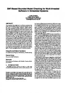
Fig. 4 demonstrates different types of possible recursive function calls up to the depth ν. Fig. 4a shows an example with a single recursive function f called two times, once from function g and once from function fmain . In this example, the calltree contains two chains of calls of function f : the first one consisting of one function call {fˆ2 }, the other consisting of ν calls: {fˆ1 , fˆ20 , ..fˆν }, where the numbers 1 and ν are recursion depths. Fig. 4b shows an example with a recursive function f called multiple times from itself (in the example, it is called 2 times). There are many chains of function calls possible for such scenario, and every one consists of at most ν calls of f , as demonstrated by a sample unwinding in the example. Notably, their unwinding depths can be different (and our algorithm will be able to detect the longest ones and stop exploring the chains for which the smaller depth is sufficient for verification). Fig. 4c shows an example with indirect recursive functions f and g, such that each function is called not by itself, but by another function that it called. In the example, both f an g are unwound at most b ν2 c times (i.e., ν times altogether).
(a)
(b)
fˆmain gˆ1 fˆ2
fˆ1
fˆmain
ˆ1 h
fˆ2�
fˆ2�
fˆ2
fˆ3
fˆ3
fˆν
fˆν�
fˆ3� � fˆν−1
fˆν−1 fˆν
0
fˆ1
1
fˆ1
gˆ1
fˆν−1
(c) fˆmain
fˆν��
fˆν���
gˆ2
2
fˆ3 �� fˆν−1
gˆν−1 fˆν
3
ν−1
ν
Figure 4: A program calltree with recursive functions unwound at most ν times: a) single recursion; b) multiple recursion; c) indirect recursion