Tile-based parallel coordinates and its application ... - Computer Science

Tile-based parallel coordinates and its application in financial visualization Jamal Alsakran* , Ye Zhao* , and Xinlei Zhao† *

Kent State University, Department of Computer Science, Kent, OH, USA † Kent State University, Department of Finance, Kent, OH, USA † Office of the Comptroller of the Currency, Washington, DC, USA ABSTRACT

Parallel coordinates technique has been widely used in information visualization applications and it has achieved great success in visualizing multivariate data and perceiving their trends. Nevertheless, visual clutter usually weakens or even diminishes its ability when the data size increases. In this paper, we first propose a tile-based parallel coordinates, where the plotting area is divided into rectangular tiles. Each tile stores an intersection density that counts the total number of polylines intersecting with that tile. Consequently, the intersection density is mapped to optical attributes, such as color and opacity, by interactive transfer functions. The method visualizes the polylines efficiently and informatively in accordance with the density distribution, and thus, reduces visual cluttering and promotes knowledge discovery. The interactivity of our method allows the user to instantaneously manipulate the tiles distribution and the transfer functions. Specifically, the classic parallel coordinates rendering is a special case of our method when each tile represents only one pixel. A case study on a real world data set, U.S. stock mutual fund data of year 2006, is presented to show the capability of our method in visually analyzing financial data. The presented visual analysis is conducted by an expert in the domain of finance. Our method gains the support from professionals in the finance field, they embrace it as a potential investment analysis tool for mutual fund managers, financial planners, and investors. Keywords: Large-size Data Visualization, Multivariate Visualization, Parallel Coordinates, Transfer Functions, Tile-based Image, Financial Visualization, Mutual Fund.

1. INTRODUCTION Parallel coordinates is a major visualization tool for multivariate data representation and correlation analysis. While it achieves success in many applications, the technique frustrates many users along the increase of the number of data items. Visual clutter appears easily and unfavorably for only a few thousands of items, due to the spatial and resolution limit of the physical display devices, as well as the perception limit of the human visual system. Actually, the challenge is posed to most other multivariate visualization techniques together with parallel coordinates. Many research studies have been conducted to overcome the problem by using aggregation and abstraction in the data processing stage, or in the visualization stage, by managing visual attributes and human perceptual factors to distinguish and emphasize interested/critical items from others acting as backgrounds. In this paper, we introduce a new tile-based density image to improve the classic pixel-based parallel coordinates. The plotting area of the whole domain is divided into tiles with a user-specified resolution. Each tile of the density image stores an intersection density – the number of data-item polylines traversing the tile. Based on such representation, we apply interactive transfer functions on the whole plotting domain to provide flexible and powerful manipulating tools, which allow users to liberally assign transparency and color of the final image according to polyline (i.e. data item) distribution features. In detail, four transfer functions are defined to project the intersection density value to three color channels (e.g. R,G,B), and opacity, which are eventually used to draw the parallel coordinates image on screen. Tile-based images, together with transfer functions, supply efficiency Further author information: (Send correspondence to Jamal Alsakran) Jamal Alsakran: E-mail: [email protected] Ye Zhao: E-mail: [email protected] Xinlei Zhao: E-mail: [email protected]

1

and flexibility in the parallel coordinates display, while typical pixel-based plot restricts the transfer function usage. It can reveal particular data information that is not clear on the pixel-based rendering. For example, by using a large tile size, users are able to read the quantitative data distribution along axes. Furthermore, the designated mosaic style visualization furnishes the final display with particular aesthetic effects. The tile-based method is not in conflict with the traditional parallel coordinates, which is actually a special case with the tile size equals to one pixel. More important, our method allows the user to interactively change the tile size (e.g. by dragging a mouse) from one pixel to large values, showing continuous displays from the classic visualization result to different tile-styled outputs. Such operation gets immediate visual feedback on screen, thanks to a very fast line-tile intersection computing method expedited by using the classic Bresenham algorithm. This realtime human-machine interaction tool greatly promotes the knowledge discovery process, since users can detect useful structural features during the smooth manipulation and adjustment. The static pixel-based polyline visualization cannot provide such experience even with an opacity mapping. This feature of our method has obtained the endorsement from domain experts as an efficient instrument to visually analyze financial data. Moreover, though the tile-based aggregation seems compromising the display of concrete polylines, it can be combined with the visualization of particular data items as a meaningful background showing global trends. Our method can also be validated by a fact that for a large data set leading to visual cluttering, the pixel-based visualization either cannot provide a clear depiction of concrete polylines. Actually, our approach provides a good scheme to study outliers, as discussed in Section 5.3. Demonstrating the benefits using our method, we provide a case study on a real world data set, the mutual fund data of the United States (U.S.) during the year 2006, to visually analyze the relations between the fund characteristics and its performance. We also show the visualization results of multiple clusters that represent fund categories. The study illustrates the contribution and one of the significant applications of our method, emerging from the collaborative work of authors from both computer science and financial economics. In summary, we improve and contribute to the parallel coordinates technique in: 1. Innovating a new tile-based density image assembling the whole plotting area of parallel coordinates, which stores polyline distribution features. This representation is more general and enhances the ability for handling large-size data and conveying more useful information, such as the quantitative data measurement along each axis. 2. Applying three color channels transfer functions together with the opacity transfer function to the tilebased density image, which define the final visualization with clear information depiction and perceptual assistance. All functions are designed with easy user interaction. 3. Providing a realtime human-interaction tool for users to continuously manipulate display results with different tile sizes, which enhances the knowledge discovery ability of parallel coordinates. 4. Coupling the tile-based visualization showing global trends with interested outliers to help users study the outliers. 5. Proposing a case study on a significant application domain - financial data visualization and analysis. The study is performed by a financial expert on a real world data set with useful discoveries, and the technique has received enthusiastic support from domain practitioners.

2. RELATED WORK Multivariate data representation, interaction and analysis are of the main challenges and tasks in information visualization. A variety of methods have been applied to tackle the problem.1 Among these methods, parallel coordinates2 has achieved a great success in many applications. An extensive survey and discussion of the method was presented by Siirtola.3 Many approaches have been proposed for reducing visual cluttering due to the large number of data items rendered as polylines in parallel coordinates. Fua et al.4 developed a multi-resolution view of the data to convey aggregation information for the resulting clusters, which made it possible for users to navigate the resulting 2

(a)

(b)

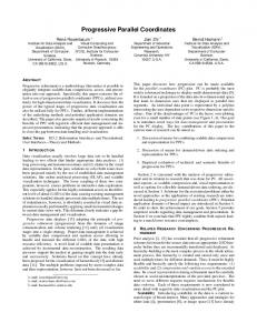
Figure 1. Visual cluttering in parallel coordinates. (a) a few data items with two attributes; (b) thousands of data items.

structure until the desired focus region and the level of detail are reached. Kosara et al.5 presented parallel sets based on a classic parallel coordinates to visualize categorical data that shows the data frequencies instead of the individual data points. Focus+context technique6 was used to enable several levels of abstraction for outliers and background trends on the basis of a novel binned data representation. Johansson et al.7 constructed highprecision textures to represent the data, and first introduced an opacity transfer function to highlight different aspects of the whole data set. This method successfully conducts a few opacity mapping methods to reveal structures of a large size data set. Comparing with the method, we apply color and opacity transfer functions to tiles, which proposes a more general framework for representing parallel coordinates plot. They also applied the approach to temporal8 and 3D parallel coordinates displays.9 Density in parallel coordinates was addressed by Miller et al.10 and Wegman et al.,11 they represented the data with a density plot to better recognize and identify patterns in heavily plotted spots. Artero et al.12 attempted to use a frequency or density information in parallel coordinates to reduce visual cluttering and emphasize significant relationships among axes. Other than parallel coordinates, Fekete et al.13 explored interactive techniques capable of handling a million items that are effectively visible and manageable on screen. Zhou et al14 proposed energy minimization to perform visual clustering, where they used transfer functions to assign opacity and colors to different clusters. The transfer functions are designed based on an average density of control points in their particular clustering algorithm. In comparison, our method generally applies the transfer functions to 2D spatial tiles, instead of polylines. Financial data analysis is a significant application domain for visual analytics, where our method is applied on data visualization and investigation. Theme River15 was applied on financial time series data to identify increases or decreases of asset prices. Time-varying indicator data was analyzed16 relying on an unsupervised clustering algorithm combined with an appropriately designed movement data visualization technique. Keim et al.17 used Growth Matrix to facilitate analysis of subinterval return rates among groups of assets. Ziegler et al.18 analyzed some of the standard statistical measures for technical financial data analysis and demonstrated the insufficient and misleading results of the real performance of one asset. Pixel-based paradigms were proposed with improved insights for asset analysis and discovery.19 Recently, A density based distribution map was proposed to visually analyze the mutual fund performance.20

3. PARALLEL COORDINATES AND VISUAL CLUTTERING Multivariate data represent and abstract information from many real world problems, which consist of a collection of data items of N attributes. The number of dimensions, N, is usually larger than three, in which case the data might be directly mapped onto 3D spatial domain, therefore, be easily understood by the human perception system. For high dimensional (i.e. hypervariate/multivariate) data with a large N, advanced representation techniques are needed to assist in human perception and promote decision making. Parallel coordinates is one of the successful techniques to visualize multivariate data, where a polyline is plotted to visualize a multivariate data item. In Fig. 1a, a small portion of the data items is visualized with two attributes. One of the main drawbacks of the parallel coordinates technique arises due to the limited size of the image or the screen. While the total number of data items increases to some level, a polyline clutter will confound the displaying information to be conveyed. For instance, one cannot detect the variation of linetraversing densities among the clutter of polylines, which is critical in knowledge discovery. Fig. 1b visualizes

3

thousands of data items with the same two attributes. Clearly, it is difficult to identify the data distribution and correlation features of lines inside the clutter on the image.

4. HANDLING LARGE SIZE DATA Visual cluttering problem arises from the inherent conflict between the limited display resource and the large size data sets. We seek to tackle the problem by organizing the whole plotting area with a more general representation - the tiles, and utilizing the human perceptual factors, i.e. three color channels and transparency, to visualize tile-based parallel coordinates images.

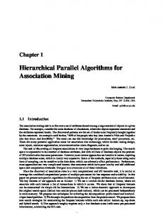
4.1 Color and Opacity Transfer Functions Successful information visualization designs have their roots in a deep understanding and effective utilization of the human perception. Our approach provides full control to users on manipulating color and opacity through transfer functions on parallel coordinates displays, and thus, constructs a solid support for advanced perceptual designs. Transfer functions are the key component in direct volume rendering, which assign local optical attributes (opacity, color, etc.) according to the density values of volume data, and have been widely and successfully applied to a variety of medical, industrial and scientific applications.21 Typical transfer functions are applied to color for dyeing and to opacity for classification. Previous work in information visualization has introduced opacity transfer function for classification,7 and utilized transfer functions to assign opacity and colors to polylines of clusters according to a particular local line density.14 In this paper, we further enhance the visualization of parallel coordinates by applying full transfer functions on the array of fragments forming the whole plotting area, in order to achieve better perceptual effects. The parallel coordinates plotting area defines an image, I(W, H), with width W and height H. In other words, the image consists of W × H fragments, and in the simplest case, a fragment coincides with a pixel. Each data item q is projected as a polyline on the image, I. For each fragment I(x, y), where 0 ≤ x < W and 0 ≤ y < H, we compute the number of lines intersecting with it, denoting as D(x, y). Thus, a polylineintersection density image D(W, H) is generated. In direct volume rendering, the density value of a volume data set is mapped to color and opacity by transfer functions. Similarly, for each fragment I(x, y), we define four transfer functions T F to determine the three color elements, R, G, B, and the opacity, O, from its density value D(x, y) as RGBO(I(x, y)) = T FRGBO (D(x, y)). Note that we use RGB color space here, however, our method can utilize other color spaces (such as HSV) in the same way. Unlike classic transfer functions in volume rendering, several practical issues arise in our implementation: (1) The range of density values is not fixed. An intersection density value D(x, y) theoretically ranges from 0 to num(q), where num(q) is the total number of data items. For a large data set with a large num(q), we can instead use a smaller value smallq, which is easily represented inside the transfer function window. In other words, we redistribute all the possible values of D(x, y) to smallq bins. Eventually, transfer functions are implemented as RGBO(I(x, y)) = T FRGBO (bin(D(x, y))), where the function bin() can be computed by spreading density values to the bins uniformly or logarithmically. (2) The number of fragments with very small value of D(x, y) is usually far larger than that with large D(x, y). For a large number of data items, most of the fragments on the image have zero or one line traversing them. Meanwhile, only a few fragments may accommodate the largest number of lines. Thus, in histogram drawing, we do not plot the number of zero intersection fragments that actually represent empty regions. Moreover, we can use a square root computation to scale the histogram value of the remains for better plotting effects. As an example, Fig. 2a shows the parallel coordinates display using the four transfer functions in comparison with the original display in Fig. 1b. The visual clutter makes it hard in Fig. 1b to identify the distribution of data item lines due to their overlapping and overcrowding. After expressing the congestion as the line-traversing densities and projecting the values to particular colors and opacities, Fig. 2a demonstrates the data distribution and correlation between the two axes in a more suitable way for the human perception. It also shows that using color together with opacity can further enhance the capability for creating good visual effects. Moreover, the

4

(a)

(b)

Figure 2. Parallel coordinates plot of Fig. 1b using transfer functions.

user-specified transfer functions intensify the existing tool with the abilities demanded by users for improving interaction with parallel coordinates. Fig. 2b is the transfer function window in which users can use a mouse to adjust the mapping functions and the fast visual feedback can help them find useful features immediately.

4.2 Tile-based Parallel Coordinates The art of mosaic is among the oldest, most durable and most functional art forms. For example, it was used in ancient Greece and Rome to adorn architectural surfaces.22 Fig. 3 shows how tiles that fit together to represent colors and shadows, leading to a vivid and spirited aesthetic sensation of the image. The mosaic-style rendering is still widely explored in modern arts, as well as in computer graphics, due to its ability on inspiring the human perception to better obtain and understand visual information. Motivated by this, we seek to further enhance the visual understanding of massive data on parallel coordinates with the tile-based method.

We use terminology, fragment, in Section 4.1 to describe applying transfer functions to the plotting domain. If simply using each fragment for each pixel in the image space, the transfer function technique is applied directly to the classic parallel coordinates. Here, we promote the traditional pixel-based perspective of plotting to a new stage, by defining each fragment to represent one tile, which is a rectangular region of the image space with a user-specified size. Users can thus have their choices to define how they want to divide the parallel coordinates image into a group of tiles, from one extreme where one tile is one pixel, to the other extreme where one tile covers the whole image space. With an appropriate small tile resolution, the quantitative visual readings along each axis are available to present Figure 3. Meditating Woman. the detail distribution of the corresponding data attribute (see the case study for This mosaic was featured in examples). the 2004 international exhibition of the Society of American Mosaic Artists. Courtesy of Rhonda Heisler Mosaic Art.

Fig. 4 demonstrates the tile-based parallel coordinates display with a predefined opacity transfer function. Fig. 4a shows a classic parallel coordinates display with about 5000 data items. Clearly, it is extremely hard to reveal the main trend of the data, or to classify the dominant relation among these dimensions. Reducing cluttering by a density-opacity mapping, Fig. 4b (top) shows the result on a pixel-based parallel coordinates display, where we adopt a square root opacity transfer function (Fig. 4b (bottom)) as in.7 It demonstrates two trends starting from the top and the bottom of the left axis, respectively. We also plot the histogram of the densities (with yellow bars), where a high-dynamic range of densities is shown. Most pixels have very small density (i.e. few passing lines) and high density pixels are very scarce. It is hard to design a good opacity mapping function based on the density information from the histogram. In comparison, Fig. 4c uses a coarser representation of the domain with a tile resolution of 30 × 30. The new histogram provides clearer data distribution information, which can better assist transfer function design. Here, we show the result with the similar opacity-only transfer function to compare with Fig. 4b. It clearly illustrates more structural features by: (1) finding another high-density trend starting from around center of the left axis; (2) revealing that more data items coming from the bottom than from the top of the left axis with darker tiles.

5

(a) Classic display (b) Resolution=450 (c) Resolution=30 Figure 4. Tile-based parallel coordinates comparing with the classic display.

4.3 Fast Computing of Line-Tile Intersection Using a tile-based image to store density values in D(W, H) requires an algorithm to compute the intersection between each line and each tile. To provide immediate visual feedback when users continuously change the tile size, a fast computing algorithm is critical for the method. A straightforward implementation that repeatedly computes intersection between each pair of line and tile has unacceptable time performance for a large data set. We thus seek to use an incremental algorithm scanning each line. This problem approximates the common problem of drawing lines on a raster pixel grid of the screen. Bresenham algorithm23 is one of the earliest algorithms developed in the field of computer graphics, as it uses only integer addition, subtraction and bit shifting all of which are very cheap operations in standard computer architectures.

Figure 5. Compute line-tile intersection by Bresenham method.

Fig. 5 demonstrates our computing process for line-tile intersection. Classic Bresenham method assumes that the computational unit is one pixel. To fully utilize the seminal algorithm, we first perform a coordinates transformation, which scales each tile to one pixel. That is, we scale a tile’s width Tx and height Ty to one unit of pixel. With the same computation, the intersection line is also scaled.

4.4 Results Fig. 6 demonstrates the tile-based parallel coordinates displays with different tile resolutions and four transfer functions. Fig. 6a shows classic parallel coordinates display without opacity difference, and as a result, with visual cluttering. The top row of Fig. 6b-d shows the visualization results of different tile resolutions, while the bottom row of them is the corresponding transfer function windows used in their generation. Tile resolution 6

(a) Classic display (b) Resolution=450 (c) Resolution=150 (d) Resolution=20 Figure 6. Tile-based parallel coordinates displays using different tile resolutions.

defines the number of tiles in x and y direction. Fig. 6b accommodates 450 tiles in both vertical and horizontal directions, in which we actually reduce the tile size to one pixel. In contrast, Fig. 6c has larger tiles with the resolution equal to 150. The latter yields better visual outcome with more obvious color levels and transitions for knowledge discovery than that of Fig. 6b, using the same transfer functions. Moreover, their histograms plotted at the bottom row clearly interpret that the low tile resolution leads to more legible intersection density distribution.

(a) Classic plot 2036

59550

101223

161006

202401

(b) Tile-based plot Figure 7. Visualization of a very large data set with 477,074 data items (U.S. stocks during years 2000 to 2007).

Fig. 6d employs very small resolution with only 20 tiles in each dimension. It can still convey the correlation information we are seeking. More important, one can further recognize the distribution of the data items along each axis: (1) most items have values at a range between 7/20 and 9/20 (the seventh to ninth tiles in yellow) of the left attribute ; and (2) most items hold values at a range of 5/20 to 7/20 of the right attribute. These data measurements cannot be easily read with a pixel-based display. Moreover, we particularly add tiny edges as 7

separators between neighboring mosaics on the low-tile-resolution images (Fig. 6d). The edges are drawn with the same transparency of the corresponding tile. This provides more artistic visual effects inspired by traditional decorative art style and enhances the understanding of the visual information. While using our system, users drag the mouse to continuously change the tile resolution, like from Fig. 6b to Fig. 6d, or vice versa. Thanks to the fast computing, the resultant images instantaneously appear on the screen along with the mouse motion. In the process, users can identify useful features not only on one static image, but also through the smooth transition among multiple images. Working on a very large data set, Fig. 7 shows the result of applying our tile-based method with transfer functions on a data set of U.S. stocks. The data set is collected on a monthly basis during the period between 2000 and 2007. It contains a very large amount of 477,074 data items. Fig. 7a presents a classic parallel coordinates view of the data set. Because the data set has nearly half a million data items, visual cluttering inevitably destroys the ability of the technique to convey any meaningful knowledge. In Fig. 7b, we show a tile-based plot with the tile resolution at 20 × 20 between each pair of adjacent dimensions. We also show the color spectrum of this plot, which is defined by the adjusted transfer functions. It describes the mapping function between the used colors and tile density values, helping us to well understand the density distribution. The new display clarifies the main trends of the data set. For example, most stocks have the volume and outstanding shares (shrOUT) in the lower half among all the possible values, and most stocks provide an inversely proportionate relation, but not very obvious, between monthly return and stock price.

5. CASE STUDY: MUTUAL FUND DATA VISUALIZATION In this section, we provide a case study using our method in financial data visualization. We investigate the U.S. mutual fund data set of the year 2006, to visually analyze the correlation between several fund characteristics and the performance (i.e. total return). Our work is a joint work among people from both computer science and finance. The case study shown here is conducted together with financial experts. It has achieved a primary support and good evaluation from the domain professionals: it has the potential to improve their state-of-the-art in massive data analysis (usually with linear regression computation). The case study description and analysis below is written by one of our authors, a professor from finance department.

5.1 Mutual Fund Data Mutual fund allows a group of investors to pool their money together and invest. The fund manager invests the fund’s assets, typically by buying stocks or bonds. In total we have 5785 funds in this study. Each data item represents one mutual fund, whose characteristics are investigated to find its correlation with the annual return. We examine the most significant characteristics including total net asset size, cash holdings, front-end load, rear-end load, expense ratios, and turnovers. As a case study, we will use our method to support knowledge discovery in this research topic of financial economics. Here, we provide a brief description of these mutual fund attributes. The total net asset size (TNA) of a mutual fund is usually measured in million U.S. dollars. Cash holding ratio (CASH) is the percentage of fund asset in the form of cash. Front-end load (FRONT LOAD) is a fee imposed upon purchase, in the percentage of fund asset. Rear-end load (REAR LOAD) is the fee imposed upon redemption, in the percentage of fund asset. Expense ratios (EXPENSES) are sometimes called the management fees, in the percentage of fund asset. Turnover rate (TURNOVER) is a measure of the fund’s transactions and is usually calculated over a year’s period. Finally, annual return (RETURN) is the percentage change in a mutual fund’s net asset value.

5.2 Front Load vs. Return Fig. 8 illustrates the visualization results of front load versus annual return, with two different tile resolutions. In classic parallel coordinates display (Fig. 8a), it seems more lines start from the top of the front load axis than from the bottom. This might result in a misleading characteristic-return analysis due to the visual clutter. With appropriate design of transfer functions (Fig. 8b), the visualization results (Fig. 8c-d) become more informative with structural emphasis by various colors and transparency. Both results illustrate that more data items are 8

from bottom than from top. Moreover, most of data items end between 0.07 and 0.26 of the return axis, revealing no obvious relation with where they come from. This indicates that (1) Most mutual funds charge about zero front load, while some mutual funds charge high front load between 4.4% to 5.8%; (2) No significant return benefits arise from such load charge difference; (3) Most funds achieve an annual return between 7% to 26%. Thus, we might conclude that it does not pay to invest in load funds.

(a) Classic display

(b) Transfer function window (c) Resolution=100 Figure 8. Visualization of front load versus return.

(d) Resolution=20

5.3 Turnover vs. Return with Outliers Our method can easily accommodate emphasized outliers together with the main trend. It can emphasize crucial data items while keeping the whole data as a background view. This is directly implemented by rendering data outliers with particular line plotting properties with some blending effects. Using our tile-based plot as a background depicting the main trend, outliers are more easily to be compared with mainstream data, leading to better understanding and analysis. In Fig. 9 we show the visualization result of mutual fund’s turnover rate versus its return. Using transfer functions to display the density of the fund distribution, the main trend is disclosed as the purple band starting from low turnover rate, ranging from 0.0 to 1.84. We render two types of outliers as solid foreground lines. The blue lines are several outliers with very Figure 9. Visualization of turnover versus return high turnover rate, and the red lines represent several outliers with outliers. Resolution=20 with the highest annual return. By comparing the outliers with the main trend, we find: (1) The mutual funds with excellent annual returns have low turnover rates; (2) On the other hand, for high turnover rate outliers, they cannot achieve high returns. The unique outlier with the highest turnover rate (at 18.34) gains its return at around 7%, even lower than the main trend return. This is discovered from an observation along the return axis on Fig. 9: intersection density of the tile adjacent to 0.07 is lower than that of the one above it.

5.4 Analyzing Statistical Regression with Visualization We use our method to visually analyze the performance of a traditional statistical method widely used by financial analysts, therefore, assist in discovering particular domain knowledge. A popular data analysis tool in financial science is the standard linear regression model that assumes a linear relation between the explanatory variables and the dependent variable .24 In this way, the relation between the return and a characteristic is defined as estimated return = coef · characteristic + interp,

9

(1)

(a) Real data

(b) Regression-estimated data Figure 10. Visualization of front load versus return.

where coef and interp are the regression coefficient and intercept, respectively. By minimizing the sum of squares of the residuals: X (estimated return − (coef · characteristic + interp))2 , (2) in the whole data set, coef and interp are determined. After computing the two values by regression, for the characteristic value of each data item, an estimated return value is achieved from Equation 1. Plotting all mutual funds with a pair of attributes: (characteristic, estimated return), the result image can be compared with the image of plotting the funds with the attributes: (characteristic, real return). This comparison provides an informative visual feedback to the regression method. In Fig. 10, we use one important characteristic of mutual fund, the total net asset (TNA), to describe the approach. Regression computation (Equation 2) gives coef = 0.003 and interp = 0.141 for the logrithmatic TNA value (Here, we use log because the TNA value span a very large range). Thus, the value of interp indicates the average return of a fund with size $1 million (log fund size = 0). Fig. 10a is the result of using real mutual fund data set. Fig. 10b replaces the real return by regression-computed estimated return. We apply the same scaling to the return axis in Fig. 10b as in Fig. 10a, which is important for correct and meaningful comparison. It manifests that the linear regression estimation approximates the relation between TNA and return in its main trend with some variations. However, some funds achieving high returns in the upper 50 percentile are not contained, which are plotted as dim tiles on Fig. 10a but not on Fig. 10b. These funds are neglected as outliers in typical regression analysis, which deserve alternative investigation other than linear regression.

5.5 Full Attributes Visualization with Outliers Fig. 11 shows our parallel coordinates display with the seven examined fund attributes. Two outliers with the two highest annual return in year 2006 are plotted separately with different colors. The red polyline represents the best performer, Dreyfus Premier Greater China B (DPCBX), which produced 85% return for investors. The purple polyline is the second-best mutual fund, Old Mutual Clay Finlay China C (OMNCX), which achieved 77% annual return. From the figure, we realize that both funds have small asset size, hold medium cash amount, charge same expense and front load, and reflect relatively low turnover rate, while they are different on rear load. It is visually clear and easy to compare them with the main trends, displayed as the mosaic-style background. The two funds generally follow the main trends on cash holdings and turnover that reflect their major managing activities in the year. They charge a little higher expenses, however, this is normal for global market funds (than U.S. domestic funds). In conclusion, the best performers’ achievement in the year 2006 has no direct relation with their fund properties and managing activities. This can attribute to the stock market booming in their investment market (China) and maybe the manager’s excellence on asset allocation.

10

Figure 11. Visualization of all the examined attributes with outliers.

5.6 Multiple Clusters Visualization Finally, we show that our method can apply independent transfer functions on different clusters. For each cluster, the plotting domain is divided into a tile-based density image. Therefore, a group of cluster images are generated. For each cluster image, its tiles are mapped to particularly-designed colors and opacities by using the transfer functions of that cluster. Finally, all tiles belonging to different clusters are blended together on the final image. As an example, Fig. 12 discovers the data distribution information among different clusters of the mutual funds. The funds are categorized into three main clusters: A. Global Equity; B. Large Capital Equity; and C. Middle/Small Capital Equity. We assign red color to cluster A; green to cluster B ; and blue to cluster C. Using opacities to emphasize high-density tiles, Fig. 12a shows the main trend of the three clusters. It can be found that cluster A charges higher expense and achieves higher return than the other two clusters, which is consistent with the behavior of funds invested in global stock market. In Fig. 12b, we adjust the transfer functions to show more data distribution information on high return funds. Clearly, most of the highest return funds belong to cluster A because of the global stock market explosion in year 2006. Global Large Middle/Small

(a) Resolution=30 (b) Resolution=60 Figure 12. Visualization of front load versus return.

6. CONCLUSION We apply novel tile-based density images to represent the plotting area of parallel coordinates, and then use color and opacity transfer functions to visualize large-size multivariate data sets for visual cluttering reduction. The transfer functions, as well as the tile resolution, are interactively designed by users. The tile-based parallel coordinates technique improves the performance, yields more controllability and promotes the visual understanding. Using the technique, we visualize and analyze a large financial data set of the 2006 U.S. equity mutual funds. It describes the power and benefits of our method as an interactive information visualization tool. Our visual analytical results also illustrate the potential of using the method in financial economics.

11

In the future, we will further enhance the ability of our parallel coordinates plotting technique. First, we will provide more assistance for user, with semi-automatic or automatic adjustment of transfer functions based on the data fact, and the spatial or topological features of plot. Second, we will conduct research on the mechanism of optimally defining a good tile size in accordance with the data features. Finally, we will extend the basic technique to more information visualization tools.

Acknowledgments The work is partially supported by National Science Foundation and the Research Council of Kent State University. We gratefully thank Nvidia for generously providing us with the graphics cards.

REFERENCES [1] Spence, R., [Information Visualization: Design for Interaction, second version ], Prentice Hall (2007). [2] Inselberg, A. and Dimsdale, B., “Parallel coordinates: a tool for visualizing multi-dimensional geometry,” Proceedings of IEEE Visualization Conference , 361–378 (1990). [3] Siirtola, H. and R¨ aih¨ a, K. J., “Interacting with parallel coordinates,” Interacting with Computers 18(6), 1278–1309 (2006). [4] Fua, Y., Ward, M., and Rundensteiner, E., “Hierarchical parallel coordinates for exploration of large datasets,” Proceedings of IEEE Visualization conference , 43–50 (1999). [5] Kosara, R., Bendix, F., and Hauser, H., “Parallel sets: Interactive exploration and visual analysis of categorical data,” IEEE Transactions on Visualization and Computer Graphics 12(4), 558–568 (2006). [6] Novotny, M. and Hauser, H., “Outlier-preserving focus+context visualization in parallel coordinates,” IEEE Transactions on Visualization and Computer Graphics 12(5), 893–900 (2006). [7] Johansson, J., Ljung, P., Jern, M., and Cooper, M., “Revealing structure within clustered parallel coordinates displays,” Proceedings of IEEE Symposium on Information Visualization , 125–132 (2005). [8] Johansson, J., Ljung, P., and Cooper, M., “Depth cues and density in temporal parallel coordinates,” Proceedings of Eurographics/IEEE-VGTC Symposium on Visualization , 35–42 (2007). [9] Johansson, J., Ljung, P., Jern, M., and Cooper, M., “Revealing structure in visualizations of dense 2d and 3d parallel coordinates,” Information Visualization 5(2), 125–136 (2006). [10] Miller, J. and Wegman, E., “Construction of line densities for parallel coordinates plots.,” in [Computing and Graphics in Statistics ], 107–123, Springer-Verlag, New York, NY, USA (1991). [11] Wegman, E. and Luo, Q., “On methods of computer graphics for visualizing densities.,” Journal of Computational and Graphical Statistics, 11, 137–162 (July 2002). [12] Artero, A., de Oliveira, M., and Levkowitz, H., “Uncovering clusters in crowded parallel coordinates visualization,” in [10th IEEE Symposium on Information Visualization ], 81–88 (2004). [13] Fekete, J. and Plaisant, C., “Interactive information visualization of a million items,” Proceedings of IEEE Symposium on Information Visualization , 117–125 (2002). [14] Zhou, H., Yuan, X., Qu, H., Cui, W., and Chen, B., “Visual clustering in parallel coordinates,” Eurographics/IEEEVGTC Symposium on Visualization 27(3), 1047–1054 (2008). [15] Havre, S., Hetzler, E., and Nowell, L., “Themeriver: Visualizing theme changes over time,” Proceedings of the International Conference Information Visualization , 115–124 (2000). [16] Schreck, T., Tekuˇsov´ a, T., Kohlhammer, J., and Fellner, D., “Trajectory-based visual analysis of large financial time series data,” ACM SIGKDD Explorations Newsletter 9(2), 30–37 (2007). [17] Keim, D. A., Nietzschmann, T., Schelwies1, N., Schneidewind, J., Schreck, T., and Ziegler, H., “A spectral visualization system for analyzing financial time series data,” Proceedings of the Eurographics/IEEE-VGTC Symposium on Visualization , 8–10 (2006). [18] Ziegler, H., Nietzschmann, T., and Keim, D. A., “Relevance driven visualization of financial performance measures,” Proceedings of the Eurographics/IEEE-VGTC Symposium on Visualization , 23–25 (2007). [19] Ziegler, H., Nietzschmann, T., and Keim, D. A., “Visual exploration and discovery of atypical behavior in financial time series data using two-dimensional colormaps,” Proceedings of the 11th International Conference Information Visualization , 308–315 (2007). [20] Alsakran, J., Zhao, Y., and Zhao, X., “Visual analysis of mutual fund performance,” Proceedings of the 13th International Conference on Information Visualization (IV09) , 252–259 (2009). [21] Pfister, H., Lorensen, B., Bajaj, C., Kindlmann, G., Schroeder, W., Avila, L. S., Martin, K., Machiraju, R., and Lee, J., “The transfer function bake-off,” IEEE Comput. Graph. Appl. 21(3), 16–22 (2001). [22] Blasi, G. and Gallo, G., “Artificial mosaics,” The Visual Computer 21(6), 373–383 (2005). [23] Bresenham, J. E., “Algorithm for computer control of a digital plotter,” in [Seminal graphics: poineering efforts that shaped the field ], 1–6, ACM, New York, NY, USA (1998). [24] Fox, J., [Applied Regression Analysis, Linear Models, and Related Methods ], Sage Publications, Inc (1997).

12