AbstractâThe usage of a network usually differs significantly at different times of a day, due to users' time-preference. This phenomenon is also prominent in the ...
Time-Dependent Network Pricing and Bandwidth Trading Libin Jiang∗ , Shyam Parekh∗† , Jean Walrand∗ ∗ Dept.
Electrical Engineering & Computer Science, University of California, Berkeley † Bell Laboratories, Alcatel-Lucent, Murray Hill, NJ 07974 Email: {ljiang,shyam,wlr}@eecs.berkeley.edu
Abstract—The usage of a network usually differs significantly at different times of a day, due to users’ time-preference. This phenomenon is also prominent in the market of “bandwidthon-demand”, since the demand is typically higher during large events. Thus, an unselfish “social planner” should deploy a proper pricing scheme to reduce congestions and achieve efficient use of the network (i.e., maximize the “social welfare”); whereas a selfish service provider (SP) can exploit the time-preference to increase its revenue. In this paper, we present a model to study the important role of time-preference in network pricing. In this model, each user chooses his access time based on his preference, the congestion level, and the price he would be charged. Without pricing, the “price of anarchy” (POA) can be arbitrarily bad. We then derive a simple pricing scheme to maximize the social welfare. Next, from the SP’s viewpoint, we consider the revenuemaximizing pricing strategy and its effect on the social welfare. We show that if the SP can differentiate its prices over different users and times, the maximal revenue can be achieved, as well as the maximal social welfare. However, if the SP has insufficient information about the users and can only differentiate its prices over the access times, then the resulting social welfare can be much less than the optimum, especially when there are many low-utility users. Otherwise, the difference is bounded and less significant.
I. I NTRODUCTION The usage of a communication network usually differs at different times of a day, because each user has its own preference over the access time, and the distribution of timepreference among a population affects the distribution of actual traffic. Also, the technological advances in networking has made it possible for ”on demand” provisioning of bandwidth for applications that require short-term bandwidth assignments, such as in the event of sporting or cultural activities. In this market, the time-preferences of the bandwidth buyers (or “users”) are especially prominent since such events draw much higher demand than usual. Also, the users’ different levels of interests on different events lead to different preferences over the time they wish to obtain the bandwidth. Without proper use of pricing, traffic delays caused by congestion during busy times can be unacceptably high, leading to inefficient utilization of the network. Intuitively, by charging higher prices during busy times, excessive congestion can be avoided, and the revenue collected by the service provider (SP) can also be increased. This work is supported by the National Science Foundation under Grant NeTS-FIND 0627161. Sincere thanks to the collaboration of Bell Labs.
A complication in this scenario is that there is no simple “demand function”, which relates the price to the user demand. The demand of the users are different at different time, but one cannot use separate demand functions for different times, because charging a higher price at a specific time will not only reduce the demand at this time, but also drive the users to migrate to other times. Therefore the demands at different times are closely correlated. In this paper, we propose a simple model to study how time-preference affects the game between the users and the service provider. Specifically, it is modeled as a selfish routing problem with user preference. We derive the pricing scheme that achieves efficient use of the network (i.e., maximizes the “social welfare”, from a social planner’s standpoint), and the one that maximize the total revenue (from a SP’s standpoint). We will show later that the resulting social welfare under the two schemes may or may not be the same, depending on how much user information the SP has. Selfish routing has been studied in various contexts. A classical model is by Wardrop [3] for the transportation network. The concept of “Price of Anarchy” (POA) was introduced in [4], measuring how bad the worst-case Nash Equilibrium (NE) is compared to Social Optimum (“SO”), in terms of some objective function (“social welfare” or “social cost”). Roughgarden et al showed that for selfish routing without pricing, and with the “social cost” is defined as the total delays of all users, the POA can be unbounded; but if the delay function is affine, the POA is upper-bounded by 4/3 [2]. A number of other works focus on networks with parallel “links”. These links are owned by a SP, or separately owned by a number of SP’s. The SP’s seek to maximize their own revenue, and are part of the game in addition to the users. Reference [5] shows that if there is one SP (monopolist), social optimum can be achieved at NE (where the SP’s revenue is maximized and the users reach Wardrop Equilibrium), if there are a large number of users and each user has a fixed amount of data to send/receive. If there are multiple SP’s (oligopolists) to compete for the users, [6] and [7] derived the POA’s with inelastic traffic and elastic traffic. In [8], Musacchio et al derived the same POA using a different approach for elastic traffic. Our model here involves parallel links (analogous to “time slots”, as detailed later), a monopolist, and assumes each user has a fixed amount of traffic (for simplicity). But
different from all the works above, each user has preference over different time slots. In other words, a user would achieve different utilities if he would choose different time slots to access the network. Reference [9] studied congestion-dependent pricing using a dynamic programming formulation. Interestingly, some conclusions of [9] are similar to ours qualitatively, although the approach used here seems more tractable. II. BASIC M ODEL AND NASH E QUILIBRIUM A. The Model and its Nash Equilibrium
st
Divide the time in a certain period (for example, one day in the case of “time-of-day pricing”; or one week in the case of “bandwidth-on-demand” trading) into N equal time slots. For simplicity, assume that each user picks one time slot to access the network, and has a fixed amount of traffic. (In the conclusion, we will discuss the extension where the users access multiple slots, and use different types of network service, such as data or voice.) Assume there are K classes of users, each of which has a profile of time-preferences. (For example, in the case of “time-of-day pricing”, office workers and college students can be defined as two different classes. In the case of “bandwidth-on-demand” trading, sports broadcasters and music broadcasters are Pntwo different classes.) The number of class-k users is dk = i=1 dik , where dik is the number of class-k users choosing slot i. Let uik be the “utility” of a class-k user if he chooses slot i, reflecting his preference. Meanwhile, the user experiences congestion delay, depending on the number of users choosing the same time slot. Then, the “payoff” for a class-k user who picks slot i is vki = uik − li (xi ) where li (·) is the congestion delay function, which PK is iassume to be increasing and convex; and xi := j=1 dj . If a particular time slot is preferred by many users, leading to high congestion, then the individual payoffs may not be high for those who choose the slot. For some users, it is possible that no matter which time slot they choose, their payoffs are negative due to large congestion delays or low utilities. If they choose not to use the network, their payoff is 0. Thus, these users will not use the network. Note that the time slots here are analogous to the parallel links in the network model ([5], [8]), since in both cases the users strategically choose from a number of options (time slots or links). But in our problem, unlike previous works, a user would get different utilities in different times due to his time perferences, a phenomenon important in network pricing and bandwidth trading. Now assume that the service provider or a social planner charges a price pik to each class-k user in slot i (If pik = 0, ∀k, i, then it is reduced to the case of no pricing.), then the payoff of this user becomes fki := uik − li (xi ) − pik and each user tries to maximize its payoff game.
We have the following about the existence of NE. Proposition 1: Given any fixed price vector p := {pik , k = 1, 2, . . . , K, i = 1, 2, . . . , N }, there exists a pure-strategy Nash equilibrium. Proof: At Nash equilibrium, the following convex optimization problem is solved: N Z xi K N X X X i i i maxd li (y)dy (uk − pk )dk −
(1) fki
in the Nash
i=1 k=1 N X dik ≤ i=1
i=1
0
dk , ∀k; dik ≥ 0, ∀k, i
(2)
PK where xi = k=1 dik is the total number of users in slot i. Indeed, the KKT condition [11] for (2) is that for each k, there exists a λk , such that ( uik − pik − li (xi ) = λk ∀dik > 0 (3) uik − pik − li (xi ) ≤ λk ∀dik = 0 This is exactly the condition for a NE. The “social welfare” V (d) is defined as the sum of the payoffs of the users and the SP (or the social planner), given an allocation d := {dik , k = 1, 2, . . . , K, i = 1, 2, . . . , N }: V (d) : =
K N X X
fki · dik +
i=1 k=1
=
K N X X
K N X X
pik dik
i=1 k=1
[uik − li (xi )] · dik
(4)
i=1 k=1
PN PK where i=1 k=1 pik dik is the revenue collected by the SP or the social planner, and note that the term is canceled in V (d). So a high value of social welfare means a good tradeoff between realizing the users’ utilities and reducing the congestions. And the “Price of Anarchy” (POA) is the ratio between the social welfare at NE (VN E := V (dN E )) and at Social Optimum (VSO := V (d∗ ), where d∗ is the maximizer of V (d)): ρ := VN E /VSO (5) B. Price of Anarchy without Pricing Without pricing, i.e., the price vector p = 0, a simple example can show that the POA is arbitrarily bad. Let there be a single class, with population d1 = 1. There is a single time slot with u1 = 1. And assume that the delay function l(x) is continuous, strictly increasing and satisfies l(0) = 0 and l(1) = 1. At the NE, all users will use the time slot, in which case the payoff of each user is u1 − l(d1 ) = 0, the same as the payoff of not using the network. Therefore the social welfare is VN E = 0. At Social Optimum (SO), the number of users in the slot, xSO , should be smaller than 1, in which case the social welfare is VSO = xSO (1 − l(xSO )) > 0. So ρ = VN E /VSO = 0. Note that this example is not contrived. Similar situation is easy to happen in practice.
III. U SING PRICING TO ACHIEVE SOCIAL OPTIMUM With the price vector p, (3) is satisfied at NE. At the SO point, the KKT condition is that for each class k, there exists a βk , such that ( ∂V (d) = uik − li (xi ) − xi · li′ (xi ) = βk ∀dik > 0 ∂dik (6) ∂V (d) = uik − li (xi ) − xi · li′ (xi ) ≤ βk ∀dik = 0 ∂di k
(7)
In other words, if the social planner sets the price as in (7), then the social optimum can be reached. Interestingly, the price does not depend on the class k and the utility uik , but only depends on the total number of users in slot i and the function li (·), which makes it easy to implement since the number of users is easy to observe. Essentially, the price can be interpreted the “externality” caused by a class-k user in slot i to other users—the existence of this user increases the delay of every other user in slot i by li′ (xi ), while the uik component of every other user is not affected. (Similar forms of pricing also appear in some other scenarios [3], [5].) IV. T HE DISCRETE CASE In the above we have assumed that there are many users, such that a single user is relatively ”small”. As a result, the population can be modeled as a continuous variable. To understand the scenario where the sizes of users are ”large”, and each user can only choose one time slot, we give a discrete formulation in the following. We will show that even if each user is priced similarly to the continuous case above, the social optimum may not be reached at some NE. Say that there are M users. Each user chooses a time slot t in {1, 2, . . . , N } to access the network. (We intentionally use different notations from the continuous case.) User i chooses the time ti to maximize ui (t) − lt (x(t)) − pt (x(t)) where x(t) =
M X
ui (t′ ) − lt′ (x(t′ ) + 1) − ui (t) + lt (x(t)) −x(t′ )[lt′ (x(t′ ) + 1) − lt′ (x(t′ ))] −[x(t) − 1][lt (x(t) − 1) − lt (x(t))] = {ui (t′ ) − lt′ (x(t′ ) + 1) − x(t′ )[lt′ (x(t′ ) + 1) − lt′ (x(t′ )]} −{ui (t) − lt (x(t)) − [x(t) − 1][lt (x(t)) − lt (x(t) − 1)]}
(6) and (3) are identical if we let pik = xi · li′ (xi )
social welfare cannot be increased. Indeed, if he makes the switch, then V is increase by
1{tj = t}
j=1
and pt (x(t)) = [x(t) − 1][lt (x(t)) − lt (x(t) − 1)]. Here, ui (t) reflects user i’s preferences. And the price p(x(t)) reflects the externality of user i if he chooses slot t. P P The social welfare is V = i ui (ti ) − t x(t)lt (x(t)). We show that every NE is ”locally” socially optimal. That is, if user i switches from its slot at NE, ti = t, to t′ , the
= {ui (t′ ) − lt′ (x(t′ ) + 1) − pt′ (x(t′ ) + 1)} −{ui (t) − lt (x(t)) − pt (x(t))} ≤ 0 where the last step follows from the fact that user i selfishly prefers slot t to slot t′ . Although the NE is locally socially optimal, it may not be globally optimal. For example, assume there are only 2 users. User 1 is in class 1, user 2 is in class 2. User 1 prefer slot 1, user 2 prefer slot 2. Let u11 = 11, u21 = 10; u12 = 10, u22 = 11. Let the delay function in both slots be l(·), and l(0) = 0, l(1) = 1, l(2) = 5. Assume now user 1 is in slot 2, while user 2 is in slot 1. Then, no one will move unilaterally. But the social optimum is achieved when they exchange the slots. The reason for the sub-optimality is the loss of convexity in this discrete model, such that the local optimum does not imply global optimum. If the user is allowed to split their traffic to more than one time slots (a reasonable assumption), then this problem will not occur even if the ”size” of each user is large. V. R EVENUE M AXIMIZATION Now we consider the pricing strategy of a revenuemaximizing SP, and how this affects the social welfare and its revenue. A. SP has full information: Differentiated prices over time and classes Under the idealized assumption that the SP has full knowledge of the users’ classes and utilities uik , he can price the users differently based on their classes and the slots they choose. Given an allocation d = {dik , k = 1, 2, . . . , K, i = 0, 1, . . . , N }, then for a class-k users in slot i, the SP can charge up to uik − li (xi ), making the user indifferent of using any slot or not using the network. Clearly, the revenue he can collect is the same as the social welfare. Therefore, when the social optimum is reached, the revenue of the SP is also maximized. In this game, the monopolist SP has complete advantages since he can extract all the values of the users based on the user information he has, whereas the payoffs of the users are zeros. Therefore in this case, the SP’s revenue is the highest among all possible pricing schemes. This is because in any other pricing scheme, (1) the social welfare must be smaller than the maximal social welfare (also the SP’s revenue) achieved
C. Differentiated prices over time: A Continuum Model and the Price of Anarchy
3.5 3
Service Provider chooses this point
2.5 u
2 1.5 1 0.5 0
0
1000
2000
3000
4000
5000
6000
7000
x
Fig. 1. Loss of social welfare, when the SP maximizes its revenue with differentiated prices over time only
The low value of social welfare (under the SP’s revenuemaximizing pricing) in the last example clearly results from the specific distribution of the user utilities. To gain more understanding of this issue, we propose a continuum model in the following, which views the whole population as a single user with a certain utility function. Then, we derive a bound on the POA (i.e., efficiency loss) under some conditions on the utility function (or equivalent, the utility distribution of the population). 1) Continuum population model: Since there is only one price for each time slot, (2) can be written as N Z xi N K N X X X X li (y)dy pi xi − maxd uik dik − st
here, and (2) SP’s revenue can not be larger than the social welfare (since part of the social welfare goes to the users).
i=1 k=1 N X dik ≤ i=1
0
dk , ∀k; dik ≥ 0, ∀k, i
(8)
Note that given xi , i = 1, 2, . . . , N , the last two terms of the objective function are fixed. Using a dynamic programming argument, if we define
B. SP has partial information: Differentiated prices over time Usually, the SP does not have full information about the users’ utilities. As a result, he may only differentiate its price over time. Unlike the previous case, maximizing revenue here is no longer the same as achieving social optimum. Let VM R be the social welfare when the SP’s revenue is maximized (where “MR” means “Maximal Revenue”. It turns out that the ratio VM R /VSO can be arbitrarily close to 0, in sharp contrast to the previous case. Consider the following example. There is only one time slot, “slot 1”, along with slot 0. And the delay function l1 (·) = 0. There is an infinite number of classes, class 1, 2..., each with a population di = 1000. Assume u11 = 3, u1i = 2i , ∀i > 1. This distribution of user utilities is shown in Fig 1, where x is the cumulative number of users and u is the utility level. The curve in Fig 1 means that there are 1000 users with utilities not less than 3; 2000 users with utilities not less than 1; 3000 users with utilities not less than 32 , etc. Since the delay function is assumed to be 0, Fig 1 can be viewed as a “demand function”: for example, if the SP charges a price of 2 3 − ǫ (where ǫ > 0 is very small), 3000 users will use the network since they will get positive payoff by doing that. (Fig 1 is also the inverse function of the complementary cumulative distribution function (c.c.d.f.) of the user utilities.) Then, if the SP charges a price p1 = u1i − ǫ, all users in class 1, 2..., i will go to slot 1. Then the revenue has many local maxima Ri = u1i · 1000 · i, ∀i = 1, 2, .... Note that R1 = 3000, Ri = 2000∀i > 1, so the price the SP charges is p1 = u11 − ǫ ≈ 3, and VM R ≈ u11 ∗ d1 = 3000. However, optimal social welfare is achieved P∞when all users are in slot 1, making VSO = 3000 + 2000 i=2 1i → ∞. Therefore, the ratio VM R /VSO can be arbitrarily close to 0.
i=1
i=1
maxd
U (x1 , x2 , . . . , xN ) := K N X X uik dik i=1 k=1
st
N X
dik ≤ dk , ∀k; dik ≥ 0, ∀k, i
i=1
K X
dik ≤ xi , ∀i
(9)
k=1
then (8) is equivalent to
maxxi ,i=1,...,N
st
U (x1 , x2 , . . . , xN ) − N Z xi N X X i li (y)dy p xi −
i=1 N X
i=1
0
xi ≤ D, xi ≥ 0, ∀i
(10)
i=1
PK where D := k=1 dk . U (x1 , x2 , . . . , xN ) is the maximal total utility of users given xi , i = 1, . . . , N . Note that it is concave according to the theory of convex optimization [11]. Under our previous assumption about classes, U is not smooth (not differentiable at some points). But if we consider a continuum of users with infinite population (i.e, the PN constraint i=1 xi ≤ D is dropped), and if the utility vector u = (u1 , u2 , . . . , uN ) of the users follow some continuous distribution f (u), then it’s reasonable to model U as a increasing, smooth, strictly-concave function. We now quantify the relationship between the marginal utility ∇U (x) and the utility distribution f (u). It is not R required that the total population f (u)du is equal to 1.
For convenience, we assume that f (u) > 0, ∀u; and there is no atom in the distribution (i.e., there exists no u′ such that the utility vectors of a positive population of users are exactly equal to u′ ). Let u ¯i be the marginal utility in slot i ¯ be the (the smallest utility among the users in slot i) , and u ¯ = ∇U (x) is also the vector of marginal utilities. Note that u vector of dual variables of problem (9) given x. Since there is no atom in the distribution f (u), one can imagine that there is an infinite number of “classes” in the population, and each class is very small and has a unique utility vector u. Since we are solving a convex optimization problem, each “class” should choose one slot, denoted as i∗ , that gives it the maximal “net utility”, i.e., i∗ = arg maxi (ui − u ¯i ), where u ¯i is also the dual variable at slot i, as mentioned above. Therefore, any user in slot i must have the following properties (Denote its utility vector as u): (a) ui ≥ u ¯i , (b) uj − u ¯ j ≤ ui − u ¯i , ∀j 6= i. So, the number of users in slot i satisfies Z ∞ fi (ui )P r{uj ≤ ui − u ¯i + u ¯j , ∀j 6= i | ui }dui (11) xi = u ¯i
where fi (·) is the marginal distribution function of the i’th element of the population’s utility vectors. ¯ to x. Denote the mapping Equation (11) maps the vector u as x = G(¯ u). Then, ¯ = G−1 (x) ∇U (x) = u which determines ∇U (x) from the distribution f (u). (G(·) is invertible since there is no “gap” in the distribution: f (u) > 0, ∀u.) R∞ When there is only one slot, from (11), x = u¯ f (u)du := G(u); then U ′ (x) = G−1 (x). For example, the curve in Fig 1 is actually U ′ (x). But given a general distribution f (u) with many slots, computing ∇U (x) may not be easy. In Section V-C3, however, we will give an example where it can be found explicitly. 2) Price of Anarchy: We now consider the price of anarchy in the game (where the SP is also a player). For convenience, let’s denote x := (x1 , x2 , . . . , xN ). social optimum (SO), we maximize V (x) := U (x) − PAt N i=1 xi · li (xi ) subject to x ≥ 0. Denote the social optimum solution as xS ≥ 0. Then, the optimality condition is that for some λ ≥ 0, ∇U (xS ) = q(xS ) − λ λ ≥ 0 λ xS = 0 T
(12)
where the i’s element of q(x) is xi · li′ (xi ) + li (xi ). If the ith element of xS , xS,i > 0, then λi = 0. If xS,i = 0, then the ith element of q(xS ) is 0. Also, we clearly have ∂U (x) ∂xi ≥ 0, ∀x ≥ 0, so λi must be 0. As a result, (12) can be simplified as ∇U (xS ) = q(xS ) (13)
To maximize the revenue (MR), on the other hand, the service provider solves maxp,x st
pT x x is an NE given p
(14)
We claim that pT x = xT [∇U (x) − l(x)], where the i’th element of l(x) is li (xi ). Recall thatPat NE, x solves (10), and N that we have dropped the constraint i=1 di ≤ D by assuming (x) that the population is infinite. If xi > 0, then ∂U ∂xi = pi + (x) li (xi ). So xi pi = xi [ ∂U ∂xi − li (xi )]. If xi = 0 (i.e., it lies at (x) the boundary of the feasible set), then ∂U ∂xi ≤ pi +li (xi ). But (x) even in this case, xi [ ∂U ∂xi − li (xi )] = 0 = xi pi . Therefore, pT x = xT [∇U (x) − l(x)]. Denote the revenue-maximization solution as xM ≥ 0. Then, the optimality condition is that for some λ ≥ 0, ∇U (xM ) + ∇2 U (xM ) · xM λ T
λ xM
= q(xM ) − λ ≥ 0 = 0
(15)
And the price (vector) charged by the SP is pM = ∇U (xM ) − l(xM ) Proposition 2: Define the price of anarchy ρ = VM R /VSO = V (xM )/V (xS ), which is the ratio between the social welfare at the revenue-maximizing point and at the social optimum point. Then we have a lower bound of ρ: ρ ≥ 2/3, under either of the following sets of conditions: (a) Every element of ∇U (x) is concave in x, and xS ≥ xM element-wise; (b) (xS −xM )T ∇U (x) is concave in x (at least for x along the line from xM to xS ). Note that condition (a) implies (b) and therefore is stronger. Remark: The two concavity conditions are somewhat abstract. But they basically means that if the low-utility users are not dominant in the population, the efficiency loss due to the SP’s selfish behavior is not too bad. (Similar assumptions are made in [7], [8] without modeling users’ time preference.) For an opposite example, consider the curve in Fig. 1, which is actually ∇U (x) = U ′ (x) in the one-dimension case. It has a “long tail” instead of being concave, i.e., there are many lowutility users. Since the SP needs to charge a relatively high price to maximize its revenue, most users (which have low utilities) can not use the network, leading to a low value of social welfare and a ρ value close to 0. With other assumptions about the tail (not necessarily the concavity assumption made here), one may be able to find other bounds of POA. The proof is in the Appendix. To give some intuition, Fig. 2 shows the simple case when there is only one time slot. The dashed curve is the marginal utility U ′ (x), which is decreasing, and is also concave by the assumption in Proposition 2. The dotted curve is the marginal cost (delay) q(x). Social Optimum is reached at point H, where U ′ (xS ) = q(xS ) (by equation (13)). Assume that D is the point that gives the maximal
φ’(x)=N⋅(1−N⋅x)1/N when N=1,2,3 N=1 N=2 N=3
3 A A
U’(x)
2.5
G M
2
x
−x U’’(x )
M
M
φ’(x)
B
D
q(x)=[x⋅l(x)]’ x
−xM U’’(xM)
1 S
H C K
1.5
0.5
F E
0
0.2
0.4
0.6
0.8
1
x
0
x
Fig. 2. Price of Anarchy is 2/3 for the simple case with only one time slot. A detailed explanation is in the text.
revenue to the SP (clearly xM > 0), then according to (15), the distance between D and E is U ′ (xS ) − q(xS ) = −xM U ′′ (xM ) − λ = −xM U ′′ (xM ) . We draw a straight line ADF with is tangent to U ′ (x) at point D. Then since the horizontal line segment BD has a length xM , and the slope of the line ADF is U ′′ (xM ), then the line segment AB also has a length of −xM U ′′ (xM ), same as DE. As a result, the two triangles ABD and DEF are identical (the line CEF is horizontal). So, the area of DEF is one half of the area of the rectangle BCED. Note that V (xS ) is the area of GKH, and V (xM ) is the area of GKED. And V (xS ) − V (xM ) is the area of DEH. Since the area of DEH is smaller than that of DEF , and the area of GKED is larger than that of BCED, therefore [V (xS ) − V (xM )]/V (xM ) ≤ 1/2, leading to the conclusion ρ = V (xM )/V (xS ) ≥ 2/3. 3) Example: Assume that the population is normalized to 1, and the delay function li (·) = 0, ∀i. Let f (u) be the distribution function of the “utility vector” of individual users. Here, we assume a uniform distribution, that is, f (u) = 1, ∀u ∈ [0, 1]N Due to the symmetry of the distribution, xM and xS must have identical elements, respectively. That is, xM = (xM , xM , . . . , xM )T , and xS = (xS , xS , . . . , xS )T , where xM and xS are the number of users in each time slot, at the point of maximal revenue and the point of social optimum respectively. (Also, xM ≤ xS .) So it suffices to analyze V (x) = U (x) when x = (x, x, . . . , x)T , i.e., in the direction of xS − xM . Denote φ(x) := U (x). Given an x = (x, x, . . . , x)T , users in the system are distributed in such a way that achieves the maximal total utility U (x), such that the number of users in each slot does not exceed x. Let u ¯i be the minimum utility of an individual user (i.e., a “marginal user”) in slot i. By symmetry, u ¯i = u ¯, ∀i,
Fig. 3. The function φ′ (x), which is proportional to (xS − xM )T ∇U (x) when x = (x, x, . . . , x)T , is concave in this example. Here we plotted φ′ (x) with N = 1, 2, 3.
where u ¯ is the common marginal utility. Using equation (11), we have Z 1 1 · P r{uj ≤ ui , ∀j 6= i | ui }dui x = xi = u ¯ Z 1 1 · uiN −1 dui = u ¯
=
1−u ¯N N
Then u ¯ = (1 − N · x)1/N When x = (x, x, . . . , x)T , since the “marginal user” in each (x) ¯, ∀i. So slot has a utility u ¯ , we have ∂U ∂xi = u φ′ (x) = N · u ¯ = N · (1 − N · x)1/N , x ∈ [0,
1 ] N
(16)
It is easy to see that φ′ (x) is concave in x for any N ≥ 1. Fig 3 shows φ′ (x) when N = 1, 2, 3. Since (xS − xM )T ∇U (x) is proportional to φ′ (x) when x = (x, x, . . . , x)T , it is concave in the direction of xS − xM . Therefore the condition of Proposition 2 is satisfied, which 2 M) indicates ρ = VV (x (xS ) ≥ 3 . Now let’s verify whether this is true in this example. The revenue of the SP is R = u ¯ ·(N ·x) = u ¯(1− u ¯N ). To maximize 1 1/N and xM = N1+1 . From R, the SP should let u ¯M = ( N +1 ) (16), we also have 1
φ(x) =
1 − (1 − N · x) N +1 1 , x ∈ [0, ] 1 N N +1 1−(
1
1 +1
)N
N +1 . On So the social welfare at xM is φ(xM ) = 1 N +1 the other hand, the social optimum is achieved when x = xS = 1 1 N , which leads to a social welfare of φ(xS ) = 1/( N + 1). Thus, 1 1 3 ρ=1−( ) N +1 ≥ N +1 4
where the equality holds with N = 1. Indeed, ρ here is above 2 3. VI. C ONCLUSION AND E XTENSIONS In this paper, we have studied a new model for timedependent pricing in the Internet. By likening different access times to different virtual links, the resulting model is similar to selfish routing and is amenable to analysis. However, different from most existing works on selfish routing, each user here has preference to different time slots. Under this model, we have shown that without pricing, the price of anarchy can be arbitrarily bad. From the SP’s perspective, if he has perfect information about the user preferences, then differentiated pricing over users and times can result in maximal revenue and also social optimum (but all the benefits go to the SP). On the other hand, if the SP does not have user information except the amount of traffic at different time slots, it can only charge different prices over times. Then the resulting equilibrium can be far from social optimal. In general, the difference is unbounded; but under some conditions on the distribution of user preferences (specifically, if the low-utility users are not too many), the social welfare is at least 2/3 of the optimal value. In this paper, we have assume that the network is composed of a single physical link (although time slots are modeled as “virtual links”). However, it can be extended to a network (owned by one SP) with multiple links inter-connected to each other, where the amount of traffic at one link is some linear combination of traffic from multiple routes, each of which traverses a number of links [10]. Assume that the users can choose both the time and physical routes to send/receive their traffic, then this is a selfish routing problem in two dimensions: times and physical routes. It is not difficult to see that the result in section III still holds: if each link charges the marginal cost according to equation (7), social optimum can be achieved. Also, the conclusion in section V-A (SP has full information) holds, and those in section V-B (SP has partial information) holds qualitatively, but possibly not quantitatively. We have also assumed that each user has a fixed amount of traffic to send, and can only choose one time slot for simplicity. The model can be extended to the case where user i can use multiple time slots, and with different types of service (for example, voice or data). To do this, define a concave N utility function, ui (si ), where si = (s1i , s2i , . . . , sN i ) ∈ R is the vector of the traffic volumns he sends/receives in each time slot. ui (si ) is not symmetric in the sense that given the i) vector si , the marginal utility at slot j, ∂usi (s is usually j i different for different j’s. This asymmetry reflects his timepreference. Also, ui (si ) takes different forms for different types of service. In this scenario, a social planner would still charge the marginal price to achieve social optimum. But when a monopolist SP tries to maximize its revenue with linear pricing, we expect that social optimum could not be achieved even if the SP knows the exact utility functions of the users, since the the revenue (price multiplied by volumn) is usually
not the same as (or “not aligned to”) the user utility. A more detailed study of this scenario is left for future research. This paper have focused on the analytical model. It is valuable to relate this model to empirical data on network usage or bandwidth trading. For example, the peak hours of network usage usually follows a certain pattern each day, and the revenue-maximizing SP is able to learn his optimal timeof-the-day prices over a period of time. So obtaining and comparing the data to our model is particularly interesting. A PPENDIX Proof of Proposition 2: Since condition (a) implies (b), we only PNprove the argument with condition (b). Define L(x) := i=1 xi · li (xi ), then V (x) = U (x) − L(x). It’s easy to see that L(x) is convex, therefore V (x) is concave. So, V (xM ) − V (0) = V (xM ) ≥ xTM ∇V (xM ) We claim that xTM ∇V (xM )
= xTM [∇U (xM ) − q(xM )] = xTM [−∇2 U (xM ) · xM ]
(17)
2
For convenience, denote s(xM ) := −∇ U (xM ) · xM . First by definition, xTM ∇V (xM ) = xTM [∇U (xM ) − q(xM )]. If the i’th element of xM , xM,i > 0, then in (15), λi = 0. So ∂U (xM ) (xM ) − (q(xM ))i = (s(xM ))i , making xM,i · [ ∂U∂x − ∂xi i (q(xM ))i ] = xM,i · (s(xM ))i . If xM,i = 0, then xM,i · (xM ) − (q(xM ))i ] = xM,i · (s(xM ))i = 0. This proves [ ∂U∂x i the above claim. So, V (xM ) ≥ −xTM ∇2 U (xM ) · xM From the concavity assumption in condition (b), we have for any x on the line segment between xM and xS , (xS − xM )T ∇U (x) ≤ (xS − xM )T ∇U (xM ) +(xS − xM )T ∇2 U (xM )(x − xM )
(18)
Now consider two integrals Z xS [∇U (x)]T dx = U (xS ) − U (xM ) xM
and
Z
xS
[∇U (xM ) + ∇2 U (xM )(x − xM )]T dx
xM
(xS − xM )T ∇U (xM ) 1 + (xS − xM )T ∇2 U (xM )(xS − xM ) 2 If we perform the integration along the line from xM to xS , then dx is proportional to xS − xM . From (18), we have [∇U (x)]T dx ≤ [∇U (xM ) + ∇2 U (xM )(x − xM )]T dx. So =
U (xS ) − U (xM ) ≤ (xS − xM )T ∇U (xM ) 1 + (xS − xM )T ∇2 U (xM )(xS − xM ) 2
It follows that V (xS ) − V (xM ) = U (xS ) − U (xM ) − [L(xS ) − L(xM )] 1 ≤ (xS − xM )T ∇U (xM ) + (xS − xM )T · 2 ∇2 U (xM )(xS − xM ) − (xS − xM )T q(xM ) Using (17) and (15), we have V (xS ) − V (xM ) ≤ (xS − xM )T ∇U (xM ) + 1 (xS − xM )T ∇2 U (xM )(xS − xM ) 2 −xTS q(xM ) + xTM [∇U (xM ) + ∇2 U (xM )xM ] ≤ (xS − xM )T ∇U (xM ) + 1 (xS − xM )T ∇2 U (xM )(xS − xM ) 2 −xTS [∇U (xM ) + ∇2 U (xM )xM ] + xTM [∇U (xM ) + ∇2 U (xM )xM ] = −(xS − xM )T ∇2 U (xM )xM + 1 (xS − xM )T ∇2 U (xM )(xS − xM ) 2 Then, consider V (xM ) − 2[V (xS ) − V (xM )] ≥ −xTM ∇2 U (xM )xM + (xS − xM )T ∇2 U (xM )(3xM − xS ) = −4xTM ∇2 U (xM )xM + 4xTS ∇2 U (xM )xM −xTS ∇2 U (xM )xS = −(xS − 2xM )T ∇2 U (xM )(xS − 2xM ) ≥ 0 where the last step follows from the fact that U (x) is concave. Therefore, 2 V (xM ) ≥ ρ= V (xS ) 3 R EFERENCES [1] Tim Roughgarden, ”The price of anarchy is independent of the network topology”, Proceedings of the thiry-fourth annual ACM symposium on Theory of computing, Montreal, Quebec, Canada, Pages: 428 - 437, Year: 2002 [2] Tim Roughgarden, ”How bad is selfish routing”, Journal of the ACM, 2002 [3] J. G. Wardrop, “Some theoretical aspects of road traffic research,” in Proceedings of the Institute of Civil Engineers, vol. 1, 1952, pp. 325– 378. [4] E. Koutsoupias, C. H. Papadimitriou, “Worst-case equilibria,” Annual Symposium on Theoretical Aspects of Computer Science, 1999. [5] Daron Acemoglu and Asuman Ozdaglar, “Flow Control, Routing, and Performance from Service Provider Viewpoint”, LIDS report, MIT, 2003 [6] Daron Acemoglu and Asuman Ozdaglar, “Competition and Efficiency in Congested Markets”, Mathematics of Operations Research, 2007 [7] Asuman Ozdaglar, “Price Competition with Elastic Traffic”, LIDS report, MIT, 2006 [8] John Musacchio and Shuang Wu, “The Price of Anarchy in a Network Pricing Game”, Allerton Conference 2007 [9] Ioannis Ch. Paschalidis, John N. Tsitsiklis, ”Congestion-Dependent Pricing of Network Service”, Networking, IEEE/ACM Transactions on, Volume 8, Issue 2, Apr 2000, Page(s):171 - 184
[10] F. P. Kelly, A.K. Maulloo and D.K.H. Tan, “Rate control in communication networks: shadow prices, proportional fairness and stability,” Journal of the Operational Research Society 49 (1998), 237-252. [11] S. Boyd and L. Vandenberghe, ”Convex Optimization”, Cambridge University Press, 2004.