Time-Domain Finite-Element Simulation of. Three-Dimensional Scattering and Radiation. Problems Using Perfectly Matched Layers. Dan Jiao, Member, IEEE, ...
296
IEEE TRANSACTIONS ON ANTENNAS AND PROPAGATION, VOL. 51, NO. 2, FEBRUARY 2003
Time-Domain Finite-Element Simulation of Three-Dimensional Scattering and Radiation Problems Using Perfectly Matched Layers Dan Jiao, Member, IEEE, Jian-Ming Jin, Fellow, IEEE, Eric Michielssen, Fellow, IEEE, and Douglas J. Riley
Abstract—An effective algorithm to construct perfectly matched layers (PMLs) for truncating time-domain finite-element meshes used in the simulation of three-dimensional (3-D) open-region electromagnetic scattering and radiation problems is presented. Both total- and scattered-field formulations are described. The proposed algorithm is based on the time-domain finite-element solution of the vector wave equation in an anisotropic and dispersive medium. The algorithm allows for the variation of the PML parameters within each element, which facilitates the efficient use of higher order vector basis functions. The stability of the resultant numerical procedure is analyzed, and it is shown that unconditionally stable schemes can be obtained. Numerical simulations of radiation and scattering problems based on both the zeroth- and higher order vector bases are presented to validate the proposed PML scheme. Index Terms—Electromagnetic scattering, electromagnetic transient analysis, finite element methods, numerical analysis.
I. INTRODUCTION
P
ERFECTLY matched layers (PMLs) are often used to implement absorbing boundary conditions (ABCs) in finite-difference time-domain (FDTD) [1]–[6] and finite-element frequency-domain (FEFD)-based codes [7]–[11] for simulating open-region wave propagation problems. Recently, a PML scheme to truncate finite-element time-domain meshes for analyzing two-dimensional (2-D) open-region electromagnetic scattering and radiation phenomena [12] was developed. In this paper, we extend this scheme to three-dimensional (3-D) problems. In contrast to the prior 2-D scheme, the 3-D algorithm proposed here is based on the exact vector wave equation in a dispersive and anisotropic medium. The proposed algorithm supports nonconstant PML parameters within each element, which facilitates the efficient utilization of higher order vector basis functions. The paper is organized as follows. First, a time-domain finite-element method (TDFEM) using PMLs is presented. An Manuscript received August 2, 2001; revised January 3, 2002. This work was supported by a Grant from the Air Force Office of Scientific Research (AFOSR) via the MURI Program under Contract F49620–96-1–0025 and a Grant from Sandia National Laboratory. D. Jiao was with the Center for Computational Electromagnetics, Department of Electrical and Computer Engineering, University of Illinois, Urbana, IL 61801 USA. She is now with Intel Corporation, Santa Clara, CA 95054 USA. J.-M. Jin and E. Michielssen are with the Center for Computational Electromagnetics, Department of Electrical and Computer Engineering, University of Illinois, Urbana-Champaign, IL 61801 USA. D. J. Riley is with the Electromagnetics and Plasma Physics Analysis Department, Sandia National Laboratories, Albuquerque, NM 87185 USA. Digital Object Identifier 10.1109/TAP.2003.809096
Fig. 1.
Illustration of solution domain truncated by PML.
approach for handling both dispersion and anisotropy within both the total- and scattered-field formulations is described, and a method for computing far-field quantities from near-field data is outlined. Next, the stability of the TDFEM-PML procedure is analyzed. Finally, numerical results are presented to demonstrate the effectiveness of the scheme. II. FORMULATION Consider the problem of modeling the electric field generated by an electric current in the presence of an object, with both the source and the object residing in a region . To formulate a finite-element scheme that permits the com, a PML is introduced outside to truncate putation of the computational domain (Fig. 1). The union of the PML reare gion and is denoted , and surfaces bounding and and , respectively. Inside the PML, the field denoted by satisfies the following second-order vector wave equation
(1) where stands for temporal convolution, stretched electric field given by
denotes the
(2) denoting temporal integration, , , and are with conductivities of PML walls perpendicular to the , , and
0018-926X/03$17.00 © 2003 IEEE
JIAO et al.: 3-D SCATTERING AND RADIATION PROBLEMS USING PMLs
axes, and tensor
297
is the time-domain counterpart of the diagonal
Here, denotes the total number of finite elements, , , , , , , and are square matrices whose elements are given by
(3) in which
(9)
are the stretching variables given by (10) (4) (11)
Obviously, (1) is also valid (except for a nonvanishing ) inside , where right-hand side (RHS) contributed by reverts to its unstretched value , and becomes the identity tensor. To seek the TDFEM solution of (1), Galerkin’s method is employed [13] to convert (1) into a matrix equation. Assuming given by an impedance boundary condition on
(5)
(12)
(13) and denote the volume integration over where element and surface integration over , respectively, and and are diagonal tensors given by
the weak-form solution satisfies
(6) denotes the vector basis function, represents where the outward unit vector normal to , and is a coefficient that specifies the impedance of the imposed boundary condi, (5) is nothing but the first-order boundary condition. If tion with the free-space impedance, which is also known as the first-order ABC. Theoretically, the perfect electrically or magnetically conducting wall can be used to terminate PML. However, both of them support cavity modes that are likely to degrade the performance of the PML, whereas with the use of an impedance boundary condition such as (5), the TDFEM solution is devoid of cavity modes. Expanding the stretched electric field as
(14) In (8), excitation vector given by
is the unknown vector,
is the
(15) (7) denoting the total number of expansion functions, and with within each assuming constant conductivities , , and element, the following ordinary differential equation is derived
(8)
and
are vectors that can be expressed as (16)
denotes the unit step function. The above convoin which lution can be recursively evaluated as described in [12] and [14] without the need to store fields of all past time steps. Secondorder accuracy is ensured by adopting a linear interpolation for the fields within each time step. It should be noted that tenare valid in the corner region of the PML. Their spesors cial cases, which include the side regions, can be handled more easily.
298
IEEE TRANSACTIONS ON ANTENNAS AND PROPAGATION, VOL. 51, NO. 2, FEBRUARY 2003
In arriving at (8), we use the fact that the time-domain councan be expressed as terpart of (17)
and , respectively, in the PML region so that the incident source vanishes therein. Assuming an impedance boundary condition on , we obtain a weak-form solution
where
(18) can be deTime-domain counterparts of terms like rived similarly. The assumption used in deriving (8) that be constant within each element can be removed. Without this assumption, the resultant ordinary differential equation reads (22) where (19) (23) where
and
are vectors given by To avoid the evaluation of the integrals on the RHS of (22), we using the same vector basis expand the incident field functions as those used to expand the unknown scattered field . As a result, we obtain the following ordinary differential equation:
(20) need to On the surface, this implies that and be recalculated each time step. In reality, however, only needs to be updated, because all spatial information can be precomputed and stored. Since the can be evaluated recursively, their update in each time step (at each integration point) can be carried out efficiently. The removal of the requirement that conductivity be constant within an element is important when higher order vector basis functions are employed to represent the unknown fields, because they allow for the use of larger element sizes. When the element sizes increase, the conductivity cannot be assumed constant anymore across an element. Therefore, the allowance of a nonconstant conductivity within each element facilitates the efficient use of higher order vector basis functions. The formulation described above is for the radiation case. When a scattering problem is considered, a scattered-field forin the mulation is employed. The scattered electric field satisfies entire computational domain
(21) denotes the incident field, and the permittivity where and permeability at the RHS reverts to its free-space values
(24) in which (25) is the projection of the incident field and the vector along each basis function, which is known and and can be efficiently updated at each time step, and are specifically assembled from their element counterparts. It remains to choose the proper spatial and temporal discretization schemes. For the spatial discretization, the unknown fields can be expanded using edge elements [15], higher order edge elements [16], or orthogonal vector basis functions [17]. For the temporal discretization, we can employ the central difference scheme, the backward difference scheme, and the Newmark method [18], [19]. In this work, both zeroth- and higher order vector elements are used to expand the unknown field. The Newmark method is employed for temporal discretization. The above TDFEM scheme calculates near-fields. To obtain is introduced inside the far-field data, an artificial boundary solution domain , which can be placed at or near the surface
JIAO et al.: 3-D SCATTERING AND RADIATION PROBLEMS USING PMLs
299
of the scatterer/radiator. The equivalent electric and magnetic and on can be determined from the currents fields calculated by the TDFEM. To compute far-field data, the following surface integrals are evaluated
(26) The scattered/radiated electric far-field is then be readily obtained as
(27) III. STABILITY ANALYSIS (a)
The stability analysis of the TDFEM-PML procedure is rather complicated. For simplicity, consider a PML wall perpendicular to the axis. The diagonal tensor in (3) reduces to (28) The ordinary differential equation resulting from the TDFEM solution becomes (29) in which
is a vector given by (30)
and
,
,
, and
are square matrices denoted by (b)
(31) Discretizing (29) in time using the Newmark method with , and performing the transform, we obtain
Fig. 2. Electric field radiated from an electric dipole. (a) Electric field E at r : z m (The normalized rms error is 0.81%.) (b) Electric field E at r : x : z m (The normalized rms error is 0.62%.)
= 0 667^ = 00 05^ + 0 02667^
For convenience, we discard the second term in (32) since it represents the contribution from loss, and hence it does not affect the stability criterion as analyzed in [20]. Replacing matrix with , and discarding the terms associated with and , we obtain (32) (34)
in which
(33) is obtained by discretizing (30) in time using the Here, backward Euler scheme instead of the central difference, since the latter can result in instability due to the appearance of term .
If the stability of the time-marching process indicated by (34) is satisfied, the stability of the process indicated by (32) is also satisfied, since the former requires a smaller time step to ensure stability. This is because the term associated with , when it is combined with matrix , increases the eigenvalue of the resultant matrix; the term associated with , when it is combined with matrix , decreases the eigenvalue of the resultant matrix, whereas the term associated with , when it is combined with matrix , increases the eigenvalue of the resultant matrix. As a
300
IEEE TRANSACTIONS ON ANTENNAS AND PROPAGATION, VOL. 51, NO. 2, FEBRUARY 2003
(a)
(b)
(c) Fig. 3. Scattering from a conducting sphere of radius 0.5 m. (a) Electric current induced at the conducting surface. (b) Far-field temporal signature. (c) Backscattered RCS.
result, we can resort to (34) instead of the complicated (32) to analyze the stability of the TDFEM-PML numerical procedure. Using the approach proposed in [20], we identify the characteristic equation of (34) as
(35) , in which denotes the eigenvalue of matrix system , the roots of (35) can which is nonnegative. When never go beyond the unit circle. Hence, the resultant numerical procedure is unconditionally stable. If we use the backward difference to discretize (29), the characteristic equation becomes
(36) The roots of the above equation are always inside the unit circle. Hence, by using the backward difference, the resultant numerical procedure is also unconditionally stable.
If we use the central difference to discretize (29), the characteristic equation becomes (37) Clearly, the roots of (37) can go beyond the unit circle in the complex plane, when varies from zero to infinity. The max, can be identified as imum value of , denoted as (38) Hence, we deduce the following stability criterion (39) represents the spectral radius of . Since in which , a time step smaller than that in free-space is required in the PML region to keep the time-marching procedure stable. In addition, the larger the conductivity is, the smaller the maximum time step has to be chosen. The above analysis can be extended to the entire PML region. The conclusion about the Newmark method and the backward
JIAO et al.: 3-D SCATTERING AND RADIATION PROBLEMS USING PMLs
301
(a)
(b)
(c) Fig. 4. Scattering from a dielectric sphere of radius 0.5 m and a relative permittivity � = 6:0. (a) Electric field E t at r = 00:04^ x 0 0:07^y 0 0:72^z m with t = 0:96^x +0:26^y +0:13^z (The normalized rms error is 0.36%.) (b) Electric field E 1 t at r = 0:079^x +0:008^y 00:61^z m with t = 00:98^x 00:08^y +0:14^z x + 0:05^y 0 0:96^z m with t = 00:89^x 0 0:08^y + 0:44^z (The normalized rms error (The normalized rms error is 0.44%.) (c) Electric field E 1 t at r = 0:05^ 1
is 0.31%.)
difference remains the same, whereas the stability criterion for the central difference becomes more complicated. This analysis is validated by our numerical experiments. IV. NUMERICAL EXAMPLES Implementations of the above scheme were applied to the study of several scattering and radiation phenomena. In all of these examples, the conductivity in the PML is assumed to have a quadratic profile, and the maximum conductivity is chosen such that the magnitude of the reflection coefficient of the corresponding PEC-backed PML at normal incidence is less than 0.0001. The first example involves an electric dipole radiating in free space. The electric current is given by
which is discretized into 7390 tetrahedral elements, yielding 9656 unknowns. The PML has a thickness of 0.25 m and is terminated by an electric wall. No impedance wall is used here since the frequencies of ’s modes are beyond the temporal m spectrum of (40). The electric fields observed at m are shown in Fig. 2 and comand pared to analytic data. The root-mean-square (rms) errors normalized by the maximum signal amplitude are 0.81 and 0.62%, respectively. Clearly, the simulation result agrees well with the exact data, which indicates that the PML effectively emulates an unbounded space. The second example involves a conducting sphere of radius 0.5 m, which is illuminated by an -polarized Neumann pulse
(40) ns, and where the computational domain
ns. It is placed at the center of of dimension 0.7 0.7 0.7 m,
(41)
302
IEEE TRANSACTIONS ON ANTENNAS AND PROPAGATION, VOL. 51, NO. 2, FEBRUARY 2003
(a)
(b)
(c) Fig. 5. Scattering from a coated sphere of radius 0.3 m with coating thickness 0.2 m and a relative permittivity � = 8:0. (a) Electric field E at r = 0:077^ x+ 0:076^y 0 0:85^z m. (The normalized rms error is 0.9%.) (b) Electric field E at r = 00:34^x 0 0:17^y 0 0:41^z m. (The normalized rms errors is 0.65%.) (c) Electric field E 1 t at r = 0:02^ x 0 0:088^y 0 0:76^z m with t = 0:94^x + 0:32^y + 0:1^z. (The normalized rms error is 1.08%.)
with parameters given by , ns, m, ns. The PML has a thickness of 0.25 m and is and placed 0.25 m away from the sphere surface. The PML is termi. The computational nated with an impedance wall with domain is subdivided into 47 524 elements, generating 59 482 unknowns. Fig. 3(a) gives the sampled electric current induced at the surface of the conducting sphere, which agrees with the exact Mie Series solution even though differentiation is used to calculate the result from the electric field. Fig. 3(b) shows the calculated far-field temporal signature. The backscatter radar cross section (RCS) is shown with respect to the electric size of the sphere in Fig. 3(c). Next, to examine the capability of the proposed method to handle materials, scattering from a dielectric sphere of radius 0.5 m and relative permittivity of 6.0 is analyzed. The PML has a thickness of 0.3 m and is placed 0.5 m away from the surface of the dielectric sphere since the dielectric sphere supports stronger surface waves than the previous conducting sphere. The computational domain is divided into 26 756 elements, yielding 32 967
unknowns. The sphere is illuminated by the Neumann pulse with parameters defined as , ns, m, ns. Fig. 4 shows the calculated electric fields at and m, m, and m, respectively, together with the exact data. In the fourth example, scattering from a coated sphere of radius 0.3 m with a coating thickness of 0.2 m and relative permittivity of 8 is analyzed. The computational domain is subdivided into 32 241 tetrahedra, yielding 40 695 unknowns. The incident Neumann pulse is identical to the previous example. The calcum, lated electric fields at m, and m are shown in Fig. 5. Again, the validity and accuracy of the proposed PML implementation are demonstrated. As noted in the figure, the rms error is 0.9, 0.65, and 1.08% at the three observation points, respectively. In contrast, when the first-order ABC is used to replace the PML, the corresponding rms error is 2.26, 2.19, and 2.29%, respectively. The computational domain used
JIAO et al.: 3-D SCATTERING AND RADIATION PROBLEMS USING PMLs
303
(a)
(a)
(b) (b) Fig. 6. Scattering from a dielectric sphere of radius 0.47 m and a relative permittivity 8.0. (a) Electric field E at = 0:71^ + 0:31^ 0:22^ m (The normalized rms error is 0.79%.) (b) Electric field at = 0:0035^ 0:056^ (The normalized rms 0:003^ 0:67^ m with = 0:97^ + 0:22^ error is 1.2%.)
r
y0
z
t
x
y0 E1t r y0 z x
z
x0
in the ABC calculation has the same size as that for the PML calculation; hence, the computation time and memory requirements are similar in both calculations. Next, to improve the accuracy and efficiency of the TDFEM simulation, we utilize higher order vector bases to represent the unknown fields. An example considered here is a dielectric sphere of radius 0.47 m. The problem is set up the same manner as in the third example except that the computational domain is coarsely discretized into 2633 tetrahedra, yielding 15 556 unknowns with the use of the first-order vector basis functions. ns and ns, The incident pulse parameters are which implies a maximum incident frequency of 600 MHz. The m and calculated electric fields at m are shown in Fig. 6. The applicability of the present algorithm to higher order vector bases is clearly demonstrated. The proposed TDFEM-PML scheme correctly characterizes the multiple interactions among the multiply reflected and creeping waves. The simulation results agree very well with the theoretical data.
Fig. 7. (a) Backscattered far-field 4�rE versus time. (b) Backscatter RCS versus the electrical size of the conducting cube (a = 1 m).
Finally, we simulate a conducting cube with a side-length of 1 m. The PML is of thickness 0.3 m, and is placed 0.5 m away from the conducting surface. The Neumann pulse is normally incident upon the cube with the pulse parameters defined by ns, ns, and m. The entire computational domain is subdivided into 6278 tetrahedra, yielding 42 994 unknowns with the use of first-order vector basis functions. The calculated far-field temporal signature is shown in Fig. 7(a), and the backscatter RCS is plotted in Fig. 7(b) versus the electrical size of the cube. The numerical simulation agrees very well with the measured data [21]. For this calculation, the total computation time is 1639 s on a DEC Alpha 667-MHz 21 264 processor, and the total memory used is 655 MB, of which 97 MB is used by the PML implementation. V. CONCLUSION This paper presented an algorithm for realizing PMLs in the TDFEM-based simulation of 3-D open-region electromagnetic scattering and radiation problems. The construction of the PML was described in detail for both the total- and scattered-field formulations. The formulations are based on the vector wave equation in an anisotropic and dispersive medium. By allowing
304
IEEE TRANSACTIONS ON ANTENNAS AND PROPAGATION, VOL. 51, NO. 2, FEBRUARY 2003
for the variation of the PML parameters within each finite element, the proposed algorithm can also make efficient use of higher order vector basis functions. The stability of the proposed TDFEM-PML numerical procedure was analyzed, and it was shown that an unconditionally stable scheme could be obtained. Numerical examples demonstrated that the proposed PML algorithm is sufficiently accurate and constitutes a viable alternative to the boundary integral-based schemes [22], [23] for the mesh truncation of open-region scattering and radiation problems.
[19] W. P. Carpes Jr, L. Pichon, and A. Razek, “A 3D finite element method for the modeling of bounded and unbounded electromagnetic problems in the time domain,” Int. J. Numer. Model., vol. 13, pp. 527–540, 2000. [20] D. Jiao and J. M. Jin, “A general approach for the stability analysis of the time-domain finite-element method,” IEEE Trans. Antennas Propagat., vol. 50, pp. 1624–1632, Nov. 2001. [21] R. P. Penno, G. A. Thiele, and K. M. Pasala, “Scattering from a perfectly conducting cube,” Proc. IEEE, vol. 77, pp. 815–823, May 1989. [22] D. Jiao, M. Lu, E. Michielssen, and J. M. Jin, “A fast time-domain finite element-boundary integral method for electromagnetic analysis,” IEEE Trans. Antennas Propagat., vol. 49, pp. 1453–1461, Oct 2001. [23] D. Jiao, A. Ergin, B. Shanker, E. Michielssen, and J. M. Jin, “A fast timedomain higher-order finite element-boundary integral method for threedimensional electromagnetic scattering analysis,” IEEE Trans. Antennas Propagat., pp. 1192–1202, Sept. 2002.
REFERENCES [1] J. Berenger, “A perfectly matched layer for the absorption of electromagnetic waves,” J. Comput. Phys., vol. 144, no. 2, pp. 185–200, 1994. [2] D. S. Katz, E. T. Thiele, and A. Taflove, “Validation and extension to three-dimensions of the Berenger PML absorbing boundary condition for FDTD meshes,” IEEE Microwave Guided Wave Lett., vol. 4, pp. 268–270, Aug. 1994. [3] C. E. Reuter, R. M. Joseph, E. T. Thiele, D. S. Katz, and A. Taflove, “Ultrawideband absorbing boundary condition for termination of waeguiding structures in FDTD simulations,” IEEE Microwave Guided Wave Lett., vol. 4, pp. 344–346, Oct. 1994. [4] W. C. Chew and W. Weedon, “A 3D perfectly matched medium from modified Maxwell’s equations with stretched coordinates,” Microwave Opt. Tech. Lett., vol. 7, no. 13, pp. 599–604, 1994. [5] S. D. Gedney, “An anisotropic perfectly matched layer-absorbing medium for the truncation of FDTD lattices,” IEEE Trans. Antennas Propagat., vol. 44, pp. 1630–1639, Dec. 1996. [6] L. Zhao and A. C. Cangellaris, “GT-PML: Generalized theory of perfectly matched layers and its application to the reflectionless truncation of finite-difference time-domain grids,” IEEE Trans. Microwave Theory Tech., vol. 44, pp. 2555–2563, Dec. 1996. [7] W. C. Chew and J. M. Jin, “Perfectly matched layers in the discretized space: An analysis and optimization,” Electromagn., vol. 16, pp. 325–340, 1996. [8] Z. S. Sacks, D. M. Kingsland, R. Lee, and J. F. Lee, “A perfectly matched anisotropic absorber for use as an absorbing boundary condition,” IEEE Trans. Antennas Propagat., vol. 43, pp. 1460–1463, Dec. 1995. [9] J. Y. Wu, D. M. Kingsland, J. F. Lee, and R. Lee, “A comparison of anisotropic PML to Berenger’s PML and its application to the finiteelement method for EM scattering,” IEEE Trans. Antennas Propagat., vol. 45, pp. 40–50, Jan. 1997. [10] M. Kuzuoglu and R. Mittra, “Investigation of nonplanar perfectly matched absorbers for finite-element mesh truncation,” IEEE Trans. Antennas Propagat., vol. 45, pp. 474–486, Mar. 1997. [11] J. M. Jin and W. C. Chew, “Combining PML and ABC for finite element analysis of scattering problems,” Microwave Opt. Tech. Lett, vol. 12, no. 4, pp. 192–197, July 1996. [12] D. Jiao and J. M. Jin, “An effective algorithm for implementing perfectly matched layers in time-domain finite-element simulation of openregion EM problems,” IEEE Trans. Antennas Propagat., vol. 50, pp. 1615–1623, Nov. 2000. [13] J. M. Jin, The Finite Element Method in Electromagnetics. New York: Wiley, 1993. [14] D. Jiao and J. M. Jin, “Time-domain finite element modeling of dispersive media,” IEEE Microwave Wireless Components Lett., vol. 11, pp. 220–222, May 2001. [15] A. Bossavit and I. Mayergoyz, “Edge elements for scattering problems,” IEEE Trans. Magn., vol. 25, pp. 2816–2821, July 1989. [16] R. D. Graglia, D. R. Wilton, and A. F. Peterson, “Higher order interpolatory vector bases for computational electromagnetics,” IEEE Trans. Antennas Propagat., vol. 45, pp. 329–341, Mar 1997. [17] D. Jiao and J. M. Jin, “Three-dimensional orthogonal vector basis functions for time-domain finite element solution of vector wave equations,” IEEE Trans. Antennas Propagat., vol. 51, pp. 59–66, Jan. 2003. [18] S. D. Gedney and U. Navsariwala, “An unconditionally stable finite-element time-domain solution of the vector wave equation,” IEEE Microwave Guided Wave Lett., vol. 5, pp. 332–334, Oct. 1995.
Dan Jiao (S’99–M’02) was born in Anhui Province, China, in 1972. She received the B.S. and M.S. degrees in electrical engineering from Anhui University, China, in 1993 and 1996, respectively, and the Ph.D. degree in electrical engineering from the University of Illinois at Urbana-Champaign (UIUC). From 1996 to 1998, she performed graduate studies at the University of Science and Technology of China, Hefei, China. From 1998 to 2001, she was a Research Assistant with the Center for Computational Electromagnetics, UIUC. In 2001, she joined Intel Corporation, Santa Clara, CA. Her current research interests include fast computational methods in electromagnetics and time-domain numerical techniques. Dr. Jiao was the recipient of the 2000 Raj Mittra Outstanding Research Award presented by the Department of Electrical and Computer Engineering, UIUC .
Jian-Ming Jin (S’87–M’89–SM’94–F’01) received the B.S. and M.S. degrees in applied physics from Nanjing University, Nanjing, China, in 1982 and 1984, respectively, and the Ph.D. degree in electrical engineering from the University of Michigan, Ann Arbor, in 1989. He is a Full Professor of electrical and computer engineering and Associate Director of the Center for Computational Electromagnetics at the University of Illinois at Urbana-Champaign (UIUC). He has authored or coauthored more than 120 papers in refereed journals and 15 book chapters. He has also authored The Finite Element Method in Electromagnetics (New York: Wiley, 1993) and Electromagnetic Analysis and Design in Magnetic Resonance Imaging (Boca Raton, FL: CRC, 1998), coauthored Computation of Special Functions (New York: Wiley, 1996), and coedited Fast and Efficient Algorithms in Computational Electromagnetics (Norwood, MA: Artech, 2001). His current research interests include computational electromagnetics, scattering and antenna analysis, electromagnetic compatibility, and magnetic resonance imaging. His name is often listed in the UIUC’s List of Excellent Instructors. He currently serves as an Associate Editor of Radio Science and is also on the Editorial Board for Electromagnetics Journal and Microwave and Optical Technology Letters. Dr. Jin is a member of Commision B of USNC/URSI, Tau Beta Pi, and International Society for Magnetic Resonance in Medicine. He was a recipient of the 1994 National Science Foundation Young Investigator Award and the 1995 Office of Naval Research Young Investigator Award. He also received the 1997 Xerox Junior Research Award and the 2000 Xerox Senior Research Award presented by the College of Engineering, University of Illinois at Urbana-Champaign, and was appointed as the first Henry Magnuski Outstanding Young Scholar in the Department of Electrical and Computer Engineering in 1998. He was a Distinguished Visiting Professor with the Air Force Research Laboratory in 1999. He served as an Associate Editor of the IEEE TRANSACTIONS ON ANTENNAS AND PROPAGATION from 1996 to 1998. He was the symposium Co-Chairman and Technical Program Chairman of the Annual Review of Progress in Applied Computational Electromagnetics in 1997 and 1998, respectively.
JIAO et al.: 3-D SCATTERING AND RADIATION PROBLEMS USING PMLs
Eric Michielssen (M’95–SM’99–F’02) received the M.S. degree in electrical engineering (summa cum laude) from the Katholieke Universiteit Leuven (KUL), Leuven, Belgium, in 1987 and the Ph.D. degree in electrical engineering from the University of Illinois at Urbana-Champaign (UIUC) in 1992. He served as a research and teaching assistant in the Microwaves and Lasers Laboratory at KUL and the Electromagnetic Communication Laboratory at UIUC from 1987 to 1988 and from 1988 to 1992, respectively. He joined the Faculty of the Department of Electrical and Computer Engineering at the UIUC, where he is now an Associate Director of the Center for Computational Electromagnetics at UIUC. He has authored or coauthored more than 70 journal papers and book chapters and more than 100 papers in conference proceedings. His research interests include all aspects of theoretical and applied computational electromagnetics. His principal research focus has been on the development of fast frequency and time domain integral-equation-based techniques for analyzing electromagnetic phenomena and the development of robust, genetic algorithm driven optimizers for the synthesis of electromagnetic devices. Dr. Michielssen received a Belgian American Educational Foundation Fellowship in 1988, and a Schlumberger Fellowship in 1990. He was the recipient of a 1994 International Union of Radio Scientists (URSI) Young Scientist Fellowship, a 1995 National Science Foundation CAREER Award, and the 1998 Applied Computational Electromagnetics Society (ACES) Valued Service Award. He was named 1999 URSI United States National Committee Henry G. Booker Fellow and selected as the recipient of the 1999 URSI Koga Gold Medal. He served as the Technical Chairman of the 1997 ACES Symposium, and currently serves on the ACES Board of Directors and as ACES Vice President. From 1997 to 1999, he was as an Associate Editor for Radio Science, and he currently is an Associate Editor for the IEEE TRANSACTIONS ON ANTENNAS AND PROPAGATION. He is a Member of the URSI Commission B.
305
Douglas J. Riley received the B.S. degree in mathematics from St. Mary’s College, MD, in 1980. He received the M.S. and Ph.D. degrees in electrical engineering from Virginia Polytechnic Institute, Blacksburg, in 1982 and 1986, respectively. In 1983, he joined Sandia National Laboratories, Albuquerque, NM, and is currently a Distinguished Member of the Technical Staff for his contributions to the development and application of time-domain methods in computational electromagnetics. His primary contributions have been in the development of hybrid (unstructured/structured) grid methods and subcellular techniques for finite-element, finite-volume, and finite-difference formulations. He has authored or coauthored more than 60 technical reports, journal articles, and conference papers in the area of computational electromagnetics.