time, parallel algorithm for solving planar Laplacians - School of ...

A linear work, O(n1/6 ) time, parallel algorithm for solving planar Laplacians∗ Ioannis Koutis

Gary L. Miller

Computer Science Department, Carnegie Mellon University, Pittsburgh, PA 15213 {ioannis.koutis,glmiller}@cs.cmu.edu

Abstract We present a linear work parallel iterative algorithm for solving linear systems involving Laplacians of planar graphs. In particular, if Ax = b, where A is the Laplacian of any planar graph with n nodes, the algorithm produces a vector x ¯ such that ||x − x ¯||A ≤ , in O(n1/6+c log(1/)) parallel time, doing O(n log(1/)) work, where c is any positive constant. One of the key ingredients of the solver, is an O(nk log2 k) work, O(k log n) time, parallel algorithm for decomposing any embedded planar graph into√ components of size O(k) that are delimited by O(n/ k) boundary edges. The result also applies to symmetric diagonally dominant matrices of planar structure. 1 Introduction Graph Laplacians owe their name to Laplace’s equation; they arise in its discretization. They are also intimately connected to electrical networks [5]. Solving Laplacians in the context of those two classical Scientific Computing applications was important enough to motivate and sustain for decades the research on multigrid methods [2]. More recently, the reduction of symmetric diagonally dominant systems to Laplacians [12], in combination with the observations of Boman et al. [1], extended the applicability of Laplacians to systems that arise when applying the finite element method to solve elliptic partial differential equations. Given the direct relationship of Laplacians with random walks on graphs [3], it shouldn’t be surprising that linear systems involving Laplacians quickly found other applications in Computer Science. Yet, when Vaidya introduced his combinatorial preconditioners for accelerating the solution of Laplacian systems [29], very few could foresee the wide arc of applications that emerged during the last few years. Laplacian solvers are now used routinely in applications that include ∗ This

work was supported in part by the National Science Foundation under grants CCR-9902091, CCR-9706572, ACI 0086093, CCR-0085982 and CCR-0122581

segmentation of medical images [11], or collaborative filtering [7]. They are also used as subroutines in eigensolvers that are needed in other algorithms for image segmentation [28], or more general clustering problems [22]. Besides the great impact on real world applications, the common thread among all these applications is that they generate graphs with millions or billions of vertices. Very often, the graphs are planar, as in the case of two dimensional elliptic partial differential equations. In several cases they additionally have a very simple structure. For example, the graphs arising in medical image segmentation are two and three dimensional weighted grids [11]. Thus, it is extremely important to design fast and practical solvers that specialize in planar graphs. The design of combinatorial preconditioners culminated in the recent breakthroughs of [27] and [6], that showed that general Laplacians can be solved in time O(n logO(1) n), and planar Laplacians can be solved in time O(n log3 n), using as preconditioners low stretch trees. The upper bound in this approach probably cannot be improved beyond O(n log n), due to the log n lower bound associated with the average stretch of spanning trees. This is known to be suboptimal for certain classes of un-weighted planar graphs, where multigrid methods work provably in linear time [2], matching up to a constant the lower bound. So, a particularly appealing question presents itself; what can be done in linear time? From a more practical point of view, one additional shortcoming of the preconditioner of [6], is that the algorithm for its construction is highly sequential. It is not known or obvious how to parallelize the algorithm in order to exploit the availability of a moderate number of processors in a parallel machine or in a distributed environment. In this paper we show that planar Laplacians can be solved with O(n) work, in O(n1/6 ) parallel time. The novel idea in our construction is to bypass the construction of the global low stretch tree for the given graph, by exploiting the combinatorial structure of the under-

lying unweighted graph. In the case of planar graphs, the graph can be decomposed into O(n/k) pieces of √ size O(k), with each piece having a boundary of O( k) vertices. Then, a proper ”miniature” preconditioner is constructed independently for each of these pieces. The global preconditioner will be the aggregation of the miniature preconditioners. Its quality will be bounded above by the quality of the worst among the miniature preconditioners. One basic problem we have to solve in the process, is the construction of a good decomposition. There is a considerable body of literature on linear work parallel algorithms for finding small vertex separators in planar graphs, including [9]. However, the algorithm and the underlying techniques are geared towards the construction of 2-way separators. The fastest known algorithms for constructing a small n/k-way separator use variants of recursive bisection and run in time O(n log n) [8, 14]. The complexity of both algorithms is due to the computation of a full tree of balanced separators, spending O(n) time for the construction of each level of the tree. We note that there is an O(n) time algorithm for constructing a full tree of separators for a planar graph [10]. However, the separators constructed in [10] are subtly different from the separators needed in [8] or [14]. Furthermore, the algorithm of [10] requires the computation of a BFS tree for the graph. It is a long standing open problem whether a BFS tree can be computed with O(n) work in o(n) parallel time. In this paper we adapt the techniques of [9], to give a linear work parallel algorithm for decomposing any planar graph into connected √ components of size O(k), that are delimited by O(n/ k) boundary edges.

better for many natural families of graphs [21, 19]. A major obstacle in their applicability as preconditioners was that the algorithm for their construction is polynomial in the size of the graph. Apart from the extra time for the design of the miniature preconditioner, one can also spend extra time for measuring its quality. With a global preconditioner, one has to assume the usually pessimistic theoretical guarantee for the quality of the preconditioner. With our approach, the actual quality can be measured easily, and the corresponding parameters in the solver can be adjusted accordingly. Testing the quality of the preconditioner is also useful when a fast algorithm for constructing the preconditioner is good on typical instances, but may occasionally fail, as it is the case with algorithms for constructing Steiner trees. Failure instances can be detected, and the more expensive accurate algorithm will be run only on them. Finally, we note that the algorithm for decomposing the graph seems to be necessary even for very simple graphs such as weighted square grids. The reason is that, whereas the square grid can be preconditioned without running the decomposition subroutine, the preconditioner undergoes a ”reduction” to a smaller graph which recursively must be preconditioned. The new smaller graph, does not inherit the nice properties of the original graph.

2 Notation and technical statements We will be considering planar weighted graphs G = (V, E, w). Throughout the paper we will assume that the given graph is connected and embedded. An embedding can be found in linear time [13], and in at most O(log2 n) parallel time, with parallel work ranging from O(n log log n) to O(n log2 n), depending on the 1.1 Implementation and practicality notes. parallel model [24, 16]. We believe that besides the theoretical improvement, There is a natural isomorphism between graphs and our method can lead to more practical implementations. their Laplacians. The Laplacian A of a graph G can An appealing characteristic of the miniaturization ap- be formed by letting A(i, j) = −wij and A(i, i) = proach is the fact that it disconnects the problem of the P wij . Conversely, given a Laplacian one can rei6=j existence of a good preconditioner from its construction. construct the graph. For this reason, we will be identiIn most applications, one is interested in solving many fying graphs with their Laplacians. It is easy to see that linear systems with a given Laplacian. The precondi- for two Laplacians A1 and A2 corresponding to graphs tioners depend only on the given graph, hence they are G1 = (V, E, w1 ) and G2 = (V, E, w2 ), the graph that constructed a single time. In those situations, it makes corresponds to A1 + A2 is G = (V, E, w1 + w2 ). The sense to spend more time on the construction of the condition number of two graphs is defined as the ratio preconditioners. This is because their quality affects λmax (A, B)/λmin (A, B), where λmax,min (A, B) are the the running time for every system that is solved. For maximum and minimum non trivial generalized eigenexample, in this paper, we use the preconditioners of values of the pair (A, B). Sm Spielman and Teng for the construction of the mini preLet A = (V, E) be a graph, and V = i=1 Vi , conditioners. However, without giving the details here, with Ai = (Vi , Ei ) being the graph induced on Vi . let us note that we can substitute them entirely with the Furthermore, assume that E = Sm Ei , and that every i=1 Steiner support trees [12, 19]. Steiner trees are usually edge lies in at most two Ai . Let W be the ”boundary” better than low stretch trees in practice, and provably set of nodes that appear in at least two Vi ’s, and

Wi = W ∩ Ai . We will call W a vertex separator that decomposes Pmthe graph into components of size maxi |Ai |. We call i=1 |Wi | the total boundary cost. Throughout the rest of paper we let k be any fixed constant. We will state the complexity of the algorithms as a function of k. The first contribution of this paper is the following theorem.

computed easily with linear work in O(log n) time. Thus ¯ is either an edge in G or an added edge. every edge in G The separator will be the boundary between a partition √ ¯ consisting of O(n/ k) edges. of the faces of G, There are two natural graphs to define on the set ¯ The first is where we connect two faces of faces F¯ of G. if they share an edge, the geometric dual, denoted by ¯ ∗ . In the second, the face intersection graph, we G Theorem 2.1. Every planar graph with n nodes has connect two faces if they share a vertex. Note that the a vertex separator W , that decomposes the graph face intersection graph is not in general planar, while into components of size O(k), with total boundary the dual is planar. We say that a set of faces in F¯ are √ cost O(n/ k). The separator can be constructed in edge/vertex connected if the corresponding induced O(k log n) parallel time doing O(nk log2 k) work in the graph in the geometric dual/face intersection graph is CREW PRAM model, or in O(kn) sequential time. connected. Frederickson [8], and –in a more general setting– Kiwi et al. [14], have given O(n log n) algorithms for constructing the partitioning. The partitioning enables the construction of a preconditioner with the following guarantees. Theorem 2.2. (Planar Ultra-Sparsify) Every planar graph A with √ n nodes has a subgraph B such that: (i) κ(A, B) ≤ k, (ii) if we apply Gaussian elimination on B by iteratively pivoting on degree one and two nodes √ only, we get a planar graph C with O(n log3 k/ k) nodes. Given the decomposition of Theorem 2.1, the embedded graphs B, C can be constructed with O(n log2 k) work, in O(k log n) parallel time. The rest of the paper is organized as follows. In Section 3 we give the proof of Theorem 2.1. In Section 4 we present the construction of the preconditioners. Finally, in Section 5 we explain how for a large enough constant k, we obtain the O(kn) time algorithm, and we show that for all larger values of k the parallel algorithm doing O(nk log2 k) work, has time complexity that quickly approaches O(n1/6 ) as k increases. The Appendix contains material that is well understood and helps to make our presentation self-contained. 3 Planar Graph Partitioning In this section we present an algorithm to partition a connected embedded planar graph G of size n into pieces √ of size at most O(k), by finding a set S of O(n/ k) edges that will be the boundaries of the pieces. Each boundary node is then incident to a number of pieces equal to the number of edges incident to it in √ S. Hence, the total cost of the boundary will be O(n/ k). The algorithm is based on an algorithm of Gazit and Miller [9]. It runs in O(k log n) parallel time, doing at most O(nk log2 k) work. ¯ be a triangulation Throughout this section we let G of G. Given the embedding, the triangulation can be

3.1 Neighborhoods and their cores. We define the vertex distance dist(f, f 0 ) between two faces f and f 0 to be one less than the minimum number of faces on a vertex connected path from f to f 0 . Since the faces are triangular, dist(f, f 0 ) is equal to the length of the shortest path from a vertex of f to a vertex of f 0 , plus one. Thus two distinct faces that share a vertex are at vertex distance one. A d-radius vertex connected ball centered at a face f ∈ F¯ , denote Bd (f ), is the set of all faces at distance at most d from f . That is, Bd (f ) = {f 0 ∈ F¯ | dist(f, f 0 ) ≤ d}. By induction on the radius of the ball, one can show that a ball forms a set of edge connected faces. We are now ready to give the definition of a k-neighborhood, and some of its consequences. Definition. The k-neighborhood of a face f ∈ F¯ Nk (f ) will consist of k faces defined as follows: (i) The ball Bd (f ) where d is the maximum d such |Bd (f )| ≤ k. (ii) The faces at distance d + 1 from f picked so that Nk (f ) remains edge connected and of size k. We call faces at a given distance from f a layer and those at distance d+1 the partial layer. We define d+1 to be the radius of Nk (f ). For each face we construct its k-neighborhood. The neighborhood of a face f that is incident to a node v of degree at least k, will have only a partial layer. The partial layer can be constructed by taking the first k faces going in a clockwise fashion around v. In order to simplify our presentation, if a face is incident to more than one nodes of degree more than k, we will construct one k-neighborhood per each such node, as described above. So, a given face may generate up to three neighborhoods. Lemma 3.1. The number of neighborhoods containing any given face is O(k log k ). Proof. We seek to bound the size of the set C of faces whose neighborhoods contain a given face f 0 . The neighborhoods are edge connected. If f 0 ∈ N , there

is an edge connected path of faces from f 0 to the center of N . There are at most 6k neighborhoods of radius r = 1 that may contain f 0 . Every neighborhood of radius r ≥ 2 that contains f 0 includes in its full layers at least one of 18k given faces in B1 (f 0 ), and B2 (f 0 ). So, from now on, we may assume that the neighborhoods are full balls. We claim that C is an edge connected set of faces. To see why, let f ∈ C, with N (f ) = Br (f ). Let h be the edge-incident face on the path from f to f 0 . We must have f 0 ∈ Br−1 (h). Let I(f ) be the S set of faces at distance 1 from f . We have Br (f ) = g∈I(f ) Br−1 (g). Since h ∈ I(f ), this implies that the radius of N (h) is at least r − 1. Hence f 0 ∈ N (h), and h ∈ C. We will find a set B of (2k)log k+1 neighborhoods that cover all the faces in C. To form B we will be removing, in rounds, sets of neighborhoods from C. We start with N (f 0 ) = B0 . Assume that in the tth round we removed a set Bt . We will let Bt+1 , be the neighborhoods of the faces that have not been covered in previous rounds, and are edge-incident to the faces in Bt . Hence |Bt+1 | ≤ 2k|Bt |. Let rt be the minimum radius over the neighborhoods in Bt . To go from f ∈ Bt to f 0 the path must go through rt−1 layers of a neighborhood N . By an N in Bt−1 , before it reaches the center of P t−1 inductive argument, this gives that rt ≥ i=0 ri ≥ t−1 2 . This implies that after d ≤ log k + 1 rounds, the process must stop because rd becomes greater than k, meaning that all neighborhoods in Bd have radius greater than k, which Pdis the maximum possible by definition. So, |C| ≤ 3 i=1 |Bt | = O(k log k+2 ). The critical fact is that each k-neighborhood Nk (f ) has a set Cf of core faces. The following key lemma concerning the cores, follows by a standard pigeon hole argument used by Lipton and Tarjan [17]. Lemma 3.2. Let Nk (f ) be a neighborhood of radius r. There exists a ball, B = Br0 (f ) such that 2(r − r0 ) + √ |∂B| ≤ 2k + 4. We call Br0 (f ) the core of Nk (f ). The importance of the cores becomes apparent in the following Lemma. Lemma 3.3. If Nk (f1 ) and Nk (f2 ) have at least one ¯ vertex in common and P is any shortest path in G from the boundary of f1 to the boundary of f2 , then the exposed part of P , that √ is the number of edges exterior to Cf1 ∪ Cf2 is at most 2k + 4. 3.2 An outline of the algorithm. With the introduction of the neighborhoods and their cores, we are ready to restate our goal for the rest of this section. We aim to find a set P of O(n/k) paths or incisions, with the following properties: (i) the removal of P

disconnects the graph into pieces of size O(k), (ii) the two endpoints of each incision P ∈ P are faces whose neighborhoods touch, so that Lemma 3.3 applies to P . Then, for every incision P with end faces f1 , f2 , we will include in the final separator S: (i) the boundaries of the cores Cf1 and Cf2 , and (ii) the exposed part of P . One way to think of this, is that we first find the incisions, and then we add the cores of their end points on top of them. Finally, we return to the graph the interior of all the cores. It then becomes clear that the final separator decomposes the graph into pieces of size O(k). Furthermore, by Lemma 3.2 the √ number of edges added the total in S per incision, is at most 2( 2k+4). Hence, √ number of edges in the final separator is O(n/ k).

N N N N N

N

N N

N

N

N N

N N

N

N

a.

N

N

N

N N

N

b.

N111 000 1111 0000 N 0000 1111 0000 1111 0000 1111 0000 1111 0000 1111 0000 1111 0000 1111

N

000 111 111 000 000 111 000 111 000 111 000 111 000 111 000 111

N

N

c.

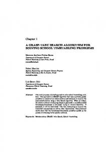
Figure 1: Steps of the algorithm. We now give a short outline of the algorithm. The first step is to obtain a maximal set I of at most n/k ¯ We will call this the face-disjoint neighborhoods in G. set of independent neighborhoods. The maximality of I will provide a good ”covering” of the graph, in the sense that the neighborhood of every face exterior to I, intersects at least one neighborhood in I. This step is shown schematically in Figure 1a and it is described formally in subsection 3.3. In the second step, we assign each exterior face to one of the neighborhoods in I, in order to decompose the graph into edgeconnected Voronoi regions of faces, each consisting of the faces assigned to one neighborhood. This step is depicted in Figure 1b and described in Section 3.4. The edges between the Voronoi regions form a planar graph that will be called the Voronoi boundary graph. The nodes in the Voronoi boundary graph with degree greater than 2 will be called Voronoi nodes. The next step will be to further decompose the graph into Voronoi-Pair regions, by finding paths between the neighborhoods and the surrounding Voronoi nodes. Two of the Voronoi-Pair regions are highlighted in Figure 1c. We give the details in Section 3.5. Finally, we separately split each Voronoi-Pair region, as described in Section 3.6. Due to lack of space, we omit the proofs of some of the easier lemmas. They are available in the full version of the paper.

3.3 Computing the set of independent neighborhoods. We say that two neighborhoods are independent if they share no faces of F¯ . Our goal will be to compute a maximal set I of independent neighborhoods. It is easy to compute I in O(kn) sequential time. For the rest of this section let us denote with |G| the number of edges of a graph G. We define the containment graph B0 to be the bipartite graph with the left side nodes corresponding to neighborhoods, and the right side nodes corresponding to faces. Any given neighborhood is joined with the k faces it contains. By construction, |B0 | ≤ 3kn. We also define the neighborhood conflict graph N (B0 ), by letting nodes correspond to neighborhoods, and edges joining neighborhoods that intersect. By Lemma 3.1, every neighborhood intersects at most O(k log k ) neighborhoods. Thus |N (B0 )| = O(k log k n). We will use a modification of Luby’s algorithm [18], that was also used in [9]. We won’t directly run the algorithm on the conflict graph. Instead, we will simulate it on the containment graph. In every round of the algorithm, every neighborhood N that remains in the graph, picks randomly a number vN in (1, n4 ). The simulation of one round will consist of k steps. In the first step each N marks its center face with vN . In every subsequent step, each N attempts to mark one face f ∈ N that has not yet been marked by N . To do this, it picks a face f 0 ∈ N that got marked by N in previous steps, and shares an edge with f . It queries the mark of f 0 . If the mark of f 0 is higher than vN , N knows that intersects a neighborhood with larger value. It thus becomes inactive and won’t try to mark other faces for the remaining steps. If the mark of f 0 is identical to vN , it goes ahead to mark f . In this way, every face receives up to 3 requests to be marked, and the related writes can be done independently. The biggest among the previous mark of f and the 3 incoming values becomes the new mark of f . After k steps, every N whose faces are marked with vN joins I. Finally, all the neighborhoods that joined I leave the graph along with their neighbors in N (B). Let Bt and N (Bt ) be the containment and conflict graphs before the tth round. It is not hard to see that the above simulation includes in I at least as many nodes as Luby’s algorithm. Hence N (Bt ) loses a constant fraction of its edges, and the algorithm finishes in O(log n) rounds. Each round can be done in O(k) parallel time. The total work is O(|Bt |) < O(|N (Bt )|). There is some d = O(log2 k) such that |N (Bd )| = O(n). Then, the total work for each of the first d rounds can be upper bounded by the size of B0 , and for the rest by the size of N (Bt ), which decreases geometrically from |N (Bd )|. Hence the total work is O(nk log2 k) .

3.4 Decomposition into Voronoi Regions. The goal of this section is to decompose the graph into edge connected Voronoi regions, each corresponding to one of the neighborhoods in I. At a high level, the approach is to find the nearest neighborhood of each exterior face f , and assign f to it. In the process, we will decompose faces that have more than one nearest neighborhood into more triangular faces, and assign these new faces to neighborhoods. Let f be an exterior face. Let ∂N denote the faces on the boundary of a neighborhood N . We define dist(f, N ) = mina∈∂N dist(f, a), and dist(f ) = minN ∈I dist(f, N ). Lemma 3.4. Let f be an exterior face of radius r. Then r ≥ dist(f ). Also, if N (a) ∈ I is such that dist(f, N (a)) = dist(f ) then N (a) and N (f ) share at least one vertex. Finally, every path of length at most dist(f )−1 starting from the boundary of f , is contained in N (f ). We now describe the algorithm. In what follows, every exterior face f will compute a labelling of each of its vertices, of the form d[a], where d will be a distance, and a the index of a neighborhood in I. The labelling will be local, and so no concurrent writes are needed. 1. Each neighborhood N (a) ∈ I marks all its faces with the index of a. Also, for each boundary vertex v of every face f , we compute the ”leftmost” (with respect to f ) BFS spanning tree of N (f ) rooted on v. 2. If a vertex v is on the boundary of some N ∈ I, it marks itself with 0 and submits clockwise the marks to its unmarked surrounding faces, so that the faces that receive the same mark are contiguous. This can be done in O(log n) time with O(n) total work. In this way, every exterior face f receives up to 3 marks through its vertices. If f receives a through vertex v, it labels v with 0[a]. Finally if f has received at least one mark, it labels with 1 each vertex that has not been marked with a 0. 3. By Lemma 3.4, to find the nearest neighborhood of an exterior face f , it is enough to consider the nodes in N (f ) that are marked with 0. First, we label each vertex v of f with the distance of the 0 vertex nearest to v, plus one. This is by definition equal to dist(f ). Let us call the vertices labelled with dist(f ) critical for f . For each critical vertex v of f , we find the preferred path P , defined as the leftmost path that (i) starts in v, (ii) reaches a vertex w in a neighborhood N ∈ I, (iii) has length dist(f ) − 1. Lemma 3.4 implies that P is contained in N (f ), and thus it can be found in O(k) time, by using the BFS computed in the previous step. The face that lies anticlockwise (with respect to w) of the last edge of P has already labelled v with 0[a], for

some a. Then, f labels v with dist(f )[a]. d [b]

d [b] b b

d+1

d+1

d+1

a

c d [c]

d+1 d [b]

d+1

b d+1

d+1 d [a]

d+1

d+1

t d+1

a a

a d [a] d [a]

d+1 d+1

d+1

a d [a]

a a

a

d+1

a

a

d+1 a

a d [a] d [a]

f1

d [a]

a

a

a

c

b b

d [a]

P1 w1

v1 dist(f1)[a] P g

b w

a

a

Figure 3: Getting one step closer to N (a).

a d [a]

v dist(f)[a]

f

d+1

d [a]

Figure 2: Breaking exterior faces. 4. One can verify that there are six different cases with respect to the type of labels that faces have computed for their vertices. These cases are shown in Figure 2, which also shows how each face is split into smaller faces that are assigned to the neighborhoods. After we split the faces that fall in to the first five cases, the remaining faces are split when needed, to make the graph triangular. All the faces assigned to a given neighborhood in N (a) ∈ I will be called the Voronoi Region of a. We claim that the above construction produces Voronoi regions that are edge connected. Lemma 3.5. All the faces that share a vertex v compute the same distance label for v. Lemma 3.6. The Voronoi regions are edge connected. Proof. By construction each neighborhood is edge connected. So, it will suffice to show that for every exterior ¯ 0 that belongs to the Voronoi region associface f 0 ∈ G ated with N (a), there is an edge connected path from f 0 to a face of N (a). Let v be the critical vertex of f 0 , ¯ It must be the case and f be the parent face of f 0 in G. that v was labelled with dist(f )[a] by f in Step 3. If dist(f ) = 1, then v is on the boundary of N (a). The algorithm ensures that there is an edge connected sequence of exterior faces surrounding v, that all marked v with 1[a]. The face on the one end of the sequence shares an edge with N (a). By the way we split the faces ¯ all the faces of G ¯ 0 that are generated inside the of G, faces in the sequence, are labelled with a. This provides the edge connected path from f 0 to N (a). Now assume dist(f ) > 1. Let P the preferred path from v. By construction, the face g on the left of the last edge of P has marked w with 0[a]. Now assume that v is not in the last edge of P , and let v1 be the ¯ vertex after v in P . We will consider the face f1 ∈ G on the left of P that includes the edge (v, v1 ), and the ¯ between f and f1 that touch v, as shown in faces of G

Figure 3. We show that these faces label v and v1 with dist(f )[a] and dist(f1 )[a] respectively. Recall that Lemma 3.5 shows that the distance labels are independent of the faces. We first show that the labels of all vertices on the arc between f and f1 must be at least equal to dist(f ). Assume for the sake of contradiction that one of these vertices, say t, is labelled with dist(f ) − 1. This means that there is a path P1 of length dist(f )−2 from t to a vertex marked with 0. The path (v, t) + P1 has length dist(f ) − 1. Then P is not the preferred path. This is a contradiction. We know already that v is critical for f . Since all the nodes of the faces between f and f1 , excluding f1 , are labelled with at least dist(f ), v is critical for them as well. Therefore, each of these faces uses independently exactly the same definition to compute the label of v in Step 3, and so the label is consistently [a]. It is easy to see that dist(f1 ) = dist(f ) − 1. Since all the other vertices of f1 are labelled with dist(f ), v1 must be labelled with dist(f1 ). The neighborhood label computed for v1 by f1 is computed by considering the last edge of the leftmost path of length dist(f ) − 2 starting from v1 . It is clear that this path is the segment of P after v1 , and thus the label is [a]. By applying this argument inductively it follows that the set of all the faces F on the left of P , mark the vertices of P with [a]. Finally consider all the faces of ¯ 0 that were generated by splitting the faces of F . First G ¯ these faces note that, by the way we split the faces of G, ¯ 0 to the face form an edge connected path from f 0 ∈ G ¯ 0 that was generated inside g. Since dist(g 0 ) = 1, g0 ∈ G we know that there is an edge connect path from it to N (a). The concatenation of the two paths forms an edge connected path from f 0 to N (a). Lemma 3.7. The set of preferred paths that reach a given N ∈ I can be used to form a BFS spanning tree of the Voronoi region of N . We call this the preferred BFS tree of the Voronoi region. Lemma 3.8. Each Voronoi region contains O(k log k ) faces.

3.5 Decomposition into Voronoi-Pair Regions. ¯ 0 by To simplify our notation, we will be denoting G ¯ We have decomposed the graph into at most n/k G. ¯ Voronoi regions. Their boundaries are edges of G. Despite the fact that these regions are edge-connected sets of faces, their boundaries may be not connected. In general, every connected region can be decomposed into a collection of simple boundary cycles, where the faces exterior to one cycle are edge-disjoint to those of another cycle. See [20] for a more complete discussion. Let C denote the set of boundary cycles of all the Voronoi regions. Any pair of boundary cycles in C, corresponding to different Voronoi regions, can share a path, a single vertex, or no vertices at all. We say that a cycle in C is non-trivial if it shares a path with at least one other cycle in C. The vertices where nontrivial cycles intersect have degree at least 3. We call these vertices the Voronoi nodes. Thinking of the simple paths between the Voronoi nodes as edges, we get a planar graph which we call the Voronoi boundary graph, denoted by GI . The graph GI will not be in general connected when the regions have disconnected boundaries. We can think of GI as a set of connected components, where each but one connected component lies inside one face of another connected component. To see this formally, pick an arbitrary ”outer” face fo of ¯ To simplify our discussion we assume wlog that the G. boundary of the region that contains fo is connected. Every region Vg has a unique external boundary cycle that lies closer to f0 . The faces enclosed by the boundary of each non-trivial internal cycle boundary of ¯ This boundary Vg form a connected component of G. is the outer face of a connected component Gc of GI . Each of the other faces of Gc correspond to the external boundary cycle of exactly one Voronoi region. It can be seen that the number of faces of GI is equal to the number of Voronoi regions that have a non-trivial external boundary. v1 g

v1

000 111 111 000 000 111 000 111

B

A

11111111111 00000000000 00000000000 11111111111 00000000000 11111111111 00000000000 11111111111 00000000000 11111111111 00000000000 11111111111 00000000000 11111111111 00000000000 11111111111 00000000000 11111111111

00000000000 11111111111 11111111111 00000000000 00000000000 11111111111 00000000000 11111111111 00000000000 11111111111 00000000000 11111111111 00000000000 11111111111 00000000000 11111111111 00000000000 11111111111 ccc

v2

g

f

f

000 111 000 111 111 000 000 111

v2

Figure 4: A Voronoi region and a Voronoi-Pair region. A topological picture of a Voronoi region with a disconnected boundary is shown in Figure 4. Searching faces out from f , the boundary of Vf is initially connected, until it reaches a saddle point, where it disconnects into two or more connected simple cycles. There

are paths from f to the saddle points that form a collection of simple cycles and decompose Vf into Voronoi subregions with simple cycle boundaries. Consider any given subregion VfA . Any point on the boundary of VfA can be reached via a shortest path from f , that lies in VfA . Provided that we are given k ≥ 3 vertices on the boundary of VfA , we can decompose VfA into k regions. The boundary of each of these smaller regions consists of one path on the boundary of VfA , and two shortest paths from its endpoints back to f . So, any segment along the boundary between two different Voronoi regions Vf , Vg , is reachable from both regions through shortest paths that lie inside the two subregions of Vf , Vg that share the given cycle, as depicted in Figure 4. This forms what we call a Voronoi-Pair region. Based on the above discussion we construct the set P of incisions and the final separator S, as described in Section 3.2. First, for each Voronoi region Vf we add shortest paths from f to the saddle points. This decomposes Vf into connected components with simple boundaries. Then, we pick three arbitrary vertices on every trivial cycle in C. Let V1 be the set of those vertices, and V2 be the Voronoi nodes. Finally, for each Voronoi region Vf we add to P the shortest paths from f to each point of its boundary which is in V1 ∪ V2 . There are at least two such points on each boundary cycle, and each Voronoi subregion is decomposed into half-Voronoi pairs. Those are coupled with half-Voronoi pairs inside the adjacent region Vg , and thus the graph is decomposed into Voronoi-Pair regions. Lemma 3.9. The number of paths added to P is at most 6n/k. Proof. Let α be the number of trivial external boundary cycles, and β be the number of non-trivial external cycles. We have α + β ≤ n/k. Let f, v, e, p be the number faces, vertices, edges, and connected components of GI . We have β = f . The number of paths to the saddle points is at most 2p + 2α. Fix a connect component Gc of GI . Let fi,c be the sizes of the faces of GI . The total P number of paths in P that are incident to Gc is i fi,c = 2ec . The number of paths to thePpoints in V1 is at most 3α. Hence, |P| ≤ 5α + 2p + 2 c ec = 5α + 2p + 2e. From Euler’s formula, we have β = 1 + p + e − v. Since 6v ≤ 4e, we have 6β = 6 + 6p + 6e − 6v ≥ 6 + 6p + 2e > 2p + 2e. So, |P| ≤ 5α + 6β ≤ 6n/k. The algorithmic details of the construction of P and S are easy and we present them in the full version of the paper. The key is that Lemma 3.3 applies to all the paths in P and these paths are constructed by using the preferred BFS trees constructed along with the Voronoi regions.

3.6 Splitting a Voronoi Pair. Let V denote the set of Voronoi-Pair regions. By Lemma 3.8, the size of each V ∈ V is bounded by O(k log k ). We can run Frederickson’s algorithm [8] on the geometric dual of each V , to √ add to the separator O(|V |)/ k edges that disconnect V into pieces of size √ number√of edges PO(k). The total added to S will be V ∈V O(|V |)/ k = O(n/ k). The P total work will be V ∈V O(|V | log |V |) ≤ n log2 k. The algorithm can be run independently on each V , so the parallel time is O(k log k ). Alternatively, we can decompose the Voronoi pairs without invoking another separator algorithm. Due to lack of space we give only a sketch of the algorithm. Let Vf and Vg be the two Voronoi regions in the pair, and Tf , Tg be their preferred BFS trees. Given a segment between two vertices w1 , w2 of the boundary, we define the weight of [w1 , w2 ] to be the total number of the nodes contained between the paths from w1 , w2 to their common ancestors, in Tf and Tg respectively. We will decompose the boundary into non-overlapping segments, such that: (i) every segment consisting of one edge has weight larger than 2k, (ii) every segment of weight less than k lies between two segments of weight larger than k, (iii) all other segments have weight between k and 2k. Let V3 be the set of the endpoints of these segments. We add to P the shortest paths from the vertices in V3 to f and g. Since the diameter of the trees is O(k), this decomposition can be done in O(k + log n) time with linear work. The total number of paths added to P is O(n/k), by construction. We are left with the segments consisting of only one edge, whose weight can be up to O(k log k ). Let M be the component defined by one such segment. We separately focus on each half of M . As implied by the proof of Lemma 3.6, along with the preferred BFS TM , we have ∗ of implicitly computed a preferred spanning tree TM ∗ the geometric dual of M . The paths of faces in TM lie along paths of TM , by construction. We will use parallel ∗ tree contraction, to find the k-critical nodes of TM in ∗ O(k) time, with O(|TM |) work (see [25] for definitions and details). The number of critical nodes is O(|M |/k). We will add to S the faces corresponding to the critical nodes. This will decompose M into O(|M |/k) pieces (called in [25] the k-bridges) of size at most O(k). The vertices contained in each of these bridges are delimited by three paths in TM . We will add these paths to P. The total number of paths added to P in this step is O(n/k) and the total work is O(kn).

√ P and W Pi = Ai ∩ W . We have i |Wi | = O(n/ k), and thus i |Ai | = O(n). Every edge of A is contained in at least one Ai , and in at most two; if it is contained in two, each cluster gets half of its weight. In this way, we get A = P A . We let Bi be the i i √ subgraph of Ai constructed by setting m = d|Ai |/ ke in Theorem 6.1. We have √ 3 |B | = |A | − 1 + |A |O(log k/ k), and κ(Ai , Bi ) = i i √i P k. The preconditioner will√be B = By i Bi . Lemma 6.1, we get κ(A, B) = k. We will be greedily removing degree one and two nodes in the interior of each Ai independently. Concretely, we let Ci = P Eliminate(Bi , Wi ) and C = C . The algorithm i i Eliminate is given in Section 6. This will provide a T partial Cholesky factorization of B = L[I, 0; 0; C]L √ . 3 By LemmaP 6.2, we have |Ci | ≤ 4(|W √ i | + |Ai | log k/ k), and |C| ≤ i |Ci | = O(n log3 k/ k). Each Bi can be constructed independently in time O(|Ai | log2 k) using Theorem P6.1. Hence, the total work for the construction of B is i |Ai | log2 k = O(n log2 k). Since A, B are embedded, C comes automatically embedded. 5

The solver and its complexity

In this section we review how the preconditioners can be used to solve a given system.

5.1 The solver. Let A be a graph with n nodes, and suppose we want to find an approximate solution x ¯ for the system Ax = b, so that kx − x ¯kA ≤ 1/2. Given an approximate solution xi , one Chebyshev iteration ([4]) obtains a better approximation xi+1 . The preconditioned Chebyshev iteration ([4]), is the Chebyshev iteration applied to the system B −1 Ax = B −1 b. Each iteration uses only matrix-vector products of the form B −1 z, which is the solution of the system By = c. p It is well known that O( κ(A, B)) Chebyshev iterations guarantee the required approximation, provided that the products B −1 z are computed exactly. In our setting, the preconditioner matrix B is a Laplacian. Let A1 be the output of algorithm Eliminate of Section 6, run on input (A, ∅). The partial Cholesky factorization of B gives B = L[I, 0; 0, A1 ]LT , where L is a lower triangular matrix with O(n) nonzero entries. One can solve By = c, by solving for z in [I, 0; 0, A1 ]z = L−1 c, and then computing y = L−T z by back-substitution. Therefore, we can solve a system in B by solving a linear system in A1 and performing O(n) additional work. However A1 may 4 Constructing the preconditioner be itself a big graph. Naturally, we can recursively In this section we show how to construct the precondi- perform preconditioned Chebyshev iterations on A1 , tioner of Theorem 2.2 given the partitioning of Theorem with a preconditioner B1 . This defines a hierarchy 2.1. Let A = {Ai } be the components of the partition, of graphs A = A0 , B0 , A1 , B1 , . . . , Ar . In [27] it was

the systems in Ar we use the parallel nested dissection algorithm of Pan and Reif [23]. The algorithm requires as input a tree of small vertex separators for Ar . This can be constructed one time, with o(n) work, and in n(1−α)/c time using Klein’s algorithm [15]. Then, the algorithm obtains a one-time factorization of Ar in polylog(n) time, with O(n3α/2 ) work, which is linear if a = 2/3. Then, every system in Ar can be solved in polylog(n) time, with O(nα ) work. The total amount of 5.2 Sequential complexity. We will assume that p for all i, 5 κ(Ai , Bi ) ln κ(Ai , Bi ) ≤ t, and |Ai |/|Ai+1 | ≥ work for solving the systems in Ar is O(n(1−α)/c nα ) = m. We let |Ar | be a constant, so that the corresponding o(n). Hence the parallel time complexity approaches systems are solved in constant time. By an easy O(n1/6 ) as c approaches 2, and the algorithm can use induction, the total number of calls to Solve with only O(n5/6 ) processors. input Ai , is ti . For each call of Solve at level i, the amount of work is O(t|Ai |) = O(tn/mi ). Assuming 6 Appendix that the sequence of graphs can be constructed in Lemma 6.1. (Splitting Lemma) Let A, B be graphs, time T , ifPt/m < 1/2, the total amount of work is with A = P Ai and B = P Bi , where for all i, Ai , Bi T + O(tn i (t/m)i ) = O(T + tn). In Theorem 2.2 are graphs on the same set of nodes. Then κ(A, B) = we can pick a value of k that satisfies t/m = 1/2 for maxi κ(Ai , Bi ). a constant t. The time to construct the hierarchy is P T = i O((k + log2 k)n/mi ) = O(kn). In comparison, The following theorem is an adaption of theorem using the construction of [27], the number of levels must Ultra-Sparsify of [27], implicitly mentioned in [6]. The be O(log P n/ log log n) and using Theorem 6.1, we have AKPW trees of [27] are replaced by the low stretch trees T = i (n/ti ) log2 (n/ti ) = O(n log3 n/ log log n). of [6]. For planar graphs sparsification, is not necessary, and this saves the logO(1) n factor in the condition 5.3 Parallel Complexity. Let us now turn our number in the original statement of the theorem. attention to the potential for parallelism in algorithm Solve. By Theorems 2.1 and 2.2, the hierarchy of Theorem 6.1. (Ultra-Sparsify) Let A be a planar graphs can be constructed with O(nk log2 k) work in graph with n nodes and m ≤ n be an integer. One can O(k log2 n) time. The algorithm can be seen as a find a subgraph B of A, with n−1+mO(log2 n log log n) sequence of Chebyshev iterations. At the end of Section edges, such that κ(A, B) ≤ n/m. B can be constructed 6 we outline how to compute the Cholesky factorization in time O(n log2 n). with O(n) in O(log n) time. Hence each iteration can Let A = (V, E) be a graph, and S ⊂ V . be done with O(n) work in O(log n) time. Both the Eliminate(A,S): If v has degree 1 and it is not in sequential and the parallel algorithms will do the same S, remove v and its adjacent edge. If v has degree 2 and number of iterations, and thus the total parallel work is it is not in S, remove v and connect its neighbors with proportional to the total sequential work. an edge. The Chebyshev iterations must be performed sequentially, so their total number is the dominating factor in the time complexity. This is dominated by the Lemma 6.2. Algorithm Eliminate returns a graph C O(tr ) iterations done at the bottom of the hierarchy. Let with at most 4(|S| + |E| − |V | + 1) nodes. m = tc . Given that |Ar | is constant, we have r ≤ logm n, It is easy to see that Eliminate preserves the and tr = O(n1/c ). Theorem 2.2 guarantees that c can be planarity and the embedding of the input graph, as taken arbitrarily close to 2, while the total work remains well as all similar structural properties. Algorithm O(n) with only a larger hidden constant. In compariEliminate can be used to derive a partial Cholesky son, the algorithm of [27] can also achieve a c arbitrarily factorization A = L[I, 0; 0, C]LT , where L has O(|V |) close to 2, but with an increase in the log terms in the non-zero entries. total work done by the algorithm. Let us now give a sketch of the computation of L. We can improve the number of Chebyshev iterations A more detailed exposition can be found, for example, while keeping the amount of work linear, by stopping the in [12]. Assume that the algorithm eliminates vertices recursion at a higher level. In the following discussion v , . . . , vk in this order, producing a sequence of graphs we omit inverse polylogarithmic factors. Let |Ar | = nα . 1 A = A0 , A1 , . . . , Ak = C, where Ai is the graph after We have r = (1 − α) logm n, and tr = n(1−α)/c . To solve the elimination of vertex vi from Ai−1 . Roughly, when shown that the following recursive algorithm obtains the required approximation: −1 Solve[A p i , b]: If i = r return Ar b. Otherwise, perform 5 κ(Ai , Bi ) ln κ(Ai , Bi ) Chebyshev iterations, with preconditioner Bi . Each time a product A−1 i+1 c is needed, use Solve[Ai+1 , c] instead. Return the last iterate.

vertex vi is eliminated, the algorithm computes a lower triangular matrix Li which has ones in the diagonal, and other non-zeros only in the ith column, at the positions of the neighbors of vi in Ai−1 . Thus, Li depends only on the graph induced on vi and its neighbors in Ai−1 . Qk We have L = i=1 Li . Assume that the eliminated vertices can be separated into sets A1 , A2 , . . . , At , such that no edges of A go between any pair of these sets. Then, if nodes i and j belong to different sets, Li and Lj commute. This can be shown formally by inspecting Q the algebraic form of Li . Hence, we can write L = i LAi , where LAi corresponds to the elimination of the nodes in Ai , and can be constructed independently from the other LAi ’s. References [1] Erik G. Boman, Bruce Hendrickson, and Stephen A. Vavasis. Solving elliptic finite element systems in near-linear time with support preconditioners. CoRR, cs.NA/0407022, 2004. [2] William L. Briggs, Van Emden Henson, and Steve F. McCormick. A multigrid tutorial: second edition. Society for Industrial and Applied Mathematics, 2000. [3] F.R.K. Chung. Spectral graph theory. Regional Conference Series in Mathematics, American Mathematical Society, 92, 1997. [4] James W. Demmel. Applied Numerical Linear Algebra. SIAM, 1997. [5] Peter G. Doyle and J. Laurie Snell. Random Walks and Electrical Networks. Mathematical Association of America, 1984. [6] Michael Elkin, Yuval Emek, Daniel A. Spielman, and Shang-Hua Teng. Lower-stretch spanning trees. In Proceedings of the 37th Annual ACM Symposium on Theory of Computing, pages 494–503, 2005. [7] Francois Fouss, Alain Pirotte, and Marco Saerens. A novel way of computing similarities between nodes of a graph, with application to collaborative recommendation. In ACM International Conference on Web Intelligence, pages 550–556, 2005. [8] Greg N. Frederickson. Fast algorithms for shortest paths in planar graphs, with applications. SIAM J. Comput., 16(6):1004–1022, 1987. [9] Hillel Gazit and Gary L. Miller. A parallel algorithm for finding a separator in planar graphs. In 28th Annual Symposium on Foundations of Computer Science, pages 238–248, Los Angeles, October 1987. IEEE. [10] Michael T. Goodrich. Planar separators and parallel polygon triangulation. J. Comput. Syst. Sci., 51(3):374–389, 1995. [11] Leo Grady. Random walks for image segmentation. EEE Trans. on Pattern Analysis and Machine Intelligence, to appear, 2006. [12] Keith Gremban. Combinatorial Preconditioners for Sparse, Symmetric, Diagonally Dominant Linear Sys-

[13] [14]

[15]

[16]

[17]

[18]

[19]

[20]

[21]

[22] [23]

[24]

[25]

[26]

[27]

[28]

[29]

tems. PhD thesis, Carnegie Mellon University, Pittsburgh, October 1996. John E. Hopcroft and Robert Endre Tarjan. Efficient planarity testing. J. ACM, 21(4):549–568, 1974. Marcos A. Kiwi, Daniel A. Spielman, and ShangHua Teng. Min-max-boundary domain decomposition. Theor. Comput. Sci., 261(2):253–266, 2001. Philip N. Klein. On Gazit and Miller’s parallel algorithm for planar separators: Achieving greater efficiency through random sampling. In Procedings of SPAA, pages 43–49, 1993. Philip N. Klein and John H. Reif. An efficient parallel algorithm for planarity. J. Comput. Syst. Sci., 37(2):190–246, 1988. R. J. Lipton and R. E. Tarjan. A planar separator theorem. SIAM J. of Applied Math., 36(2):177–189, April 1979. Michael Luby. A simple parallel algorithm for the maximal independent set problem. SIAM J. Comput., 15(4):1036–1053, 1986. Bruce M. Maggs, Gary L. Miller, Ojas Parekh, R. Ravi, and Shan Leung Maverick Woo. Finding effective support-tree preconditioners. In Procideengs of SPAA, pages 176–185, 2005. Gary L. Miller. Finding small simple cycle separators for 2-connected planar graphs. Journal of Computer and System Sciences, 32(3):265–279, June 1986. invited publication. Gary L. Miller and Peter C. Richter. Lower bounds for graph embeddings and combinatorial preconditioners. In Procedings of SPAA, pages 112–119, 2004. A. Ng, M. Jordan, and Y. Weiss. On spectral clustering: Analysis and an algorithm, 2001. Victor Y. Pan and John H. Reif. Fast and efficient parallel solution of sparse linear systems. SIAM J. Comput., 22(6):1227–1250, 1993. Vijaya Ramachandran and John H. Reif. Planarity testing in parallel. J. Comput. Syst. Sci., 49(3):517– 561, 1994. Margaret Reid-Miller, Gary L. Miller, and Francesmary Modugno. List ranking and parallel tree contraction. In Synthesis of Parallel Algorithms, pages 115–194. Morgan Kaufmann, 1993. R.E. Tarjan R.J. Lipton and D. Rose. Generalized nested dissection. SIAM Journal of Numerical Analysis, 16:346–358, 1979. Daniel A. Spielman and Shang-Hua Teng. Nearlylinear time algorithms for graph partitioning, graph sparsification, and solving linear systems. In Proceedings of the 36th STOC, pages 81–90, June 2004. David Tolliver and Gary L. Miller. Graph partitioning by spectral rounding: Applications in image segmentation and clustering. In CVPR, 2006. P.M. Vaidya. Solving linear equations with symmetric diagonally dominant matrices by constructing good preconditioners. A talk based on this manuscript, October 1991.