Difference Time Domain Method. Roberto Sorrentino, Luca Roselli, and Paolo Mezzanotte. Abstrucf- A simple modification of Yee's FDTD algorithm allows one ...
I
IEEE MICROWAVE AND GUIDED WAVE
402
LETTERS. VOL.
3 , NO. I I , NOVEMBER 1993
Time Reversal in Finite Difference Time Domain Method Roberto Sorrentino, Luca Roselli, and Paolo Mezzanotte
Abstrucf- A simple modification of Yee's FDTD algorithm allows one to reverse the time direction in FDTD simulation in much the same way as with TLM method. Numerical microwave synthesis is therefore also possible by reversing the time in the FDTD algorithm.
I. INTRODUCTION
T
HE possibility of reversing the time in the numerical simulation of microwave structures using the TLM method has been recently pointed out 121. The ultimate objective is the numerical synthesis of a microwave structure starting from its desired response. This letter shows that time reversal is also possible in the FDTD technique, thus confirming the substantial equivalence with TLM and opening the possibility of numerical microwave synthesis by time reversal in FDTD method. 11. TIME REVERSAL FDTD ALGORITHM
The Maxwell equations discretized using the Yee's algorithm [ l ] are amenable to the time-reverse computation. For simplicity we consider here the 2-D formulation. The 3-D case can be obtained by straightforward modifications. In 2-D, the discretized TE Cartesian Maxwell equations are
i.j+ i)
H:++ (if
=
(;+ 2.,J+ !j)
H:-'
-
-2-A r ( H ,r L + + ( i + - , j +. AI
-H:+'(i+;,j-;)).
In these formulas Ar Ax and Ay are the time and space discretizations respectively, Z is the intrinsic impedance of the medium. Similar formulas hold for the TM case. According to (l), the computation of H and E fields is performed according to the following sequence: 1) Starting from the H-field at the time instant t = 71 - l / 2 and the E-field at the time instant t = n, the updated H-field at t = 7~ l / 2 is computed. 2) Next, the E-field at t = n + 1 are computed from the Efield at the previous instant t = n and the just computed H-field at f, = 71 1/2. To reverse the time direction we need to reverse the sequence of the above computations; i.e., we need to compute E,t and H 7 1 - 1 / 2 starting from H n + 1 / 2 and En+i,~~~~~i~~ (1) can easily be arranged to obtain
+
+
E: (I+ ; . j )
E;+'(i
+i.j)
= E,"+1(I.)
+
=
2 ( E : ( i + 1.;j + 1) ZA:c (I.i+
i))
E; ( i . j
! j . j + 1)
+ "(.;(i+
+
i)
1)
i,,. t) 1))
+zA T ( H ,n + + ( ,I. + - ] + a:Y -H:++ ( i + ; , j
Z4Y
-
+i.j)
= Ejl ( i
+1.j)
+ Z*
(H"+'
a:Y
(i
+ i . , j+
i) -
E;+l ( i , j
+
1)
(1)
1 .
-E,;
E,"+l(i
1)
= E; ( i . j
+
i)
"I'(i. j
+ ;)) I .
MAnuscript received June 8, 1993. The authors are with the Istituto di Elettronica, Universita di Perugia, Perugia, Italy. IEEE Log Number 9213205.
1051-8207/93$03.00 0 1993 IEEE
IEEE MICROWAVE AND GUIDED WAVE LETTERS, VOL. 3 . NO 1 I , NOVEMBER 1993
403
(C)
(C)
(d)
(d)
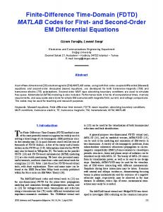
Fig. 2. Propagation of a Gaussian impulse in a parallel plate waveguide. (a), (b) Loaded with a metal septum at t = 70 and t = 110 time step. (c), (d) Unloaded at the same instant.
Fig. 1. Reconstruction of an impulsive source. (a), (b). and (c) Forward evaluation at three successive time instants. (d) Reconstructed pulse obtained by the reverse simulation.
The above equations are to be applied to compute the field components at previous instants from those at future instants at any point either internal or located at a perfect reflecting boundary (e.g. perfect conductor). Special care has to be taken when the structure is partially or totally bounded by absorbing boundaries. In the time-reverse simulation, the absorbing walls become “injecting walls”; i.e., energy is injected to the structure from the boundaries. In the forward simulation, the E M field impinges on to the absorbing boundary producing an outward power flow, thus, in the backward simulation, the same amount of power has to be reinjected in the structure. In other words, the absorbing boundaries become active boundaries, thus playing the role of a source. To implement the time reversal it is therefore necessary to know the time evolution of the field at the “active” boundary. This can be the result of either a forward simulation previously performed or some sort of a priori assumption in a synthesis procedure. 111. RECONSTRUCTION OF AN IMPULSIVE POINT SOURCE
Similarly to [2], we have first checked the validity of the above algorithm with a simple numerical experiment consisting in the reconstruction of a point source from its radiated field. An irregularly shaped 2-D structure bounded by perfectly conducting walls was excited by an impulsive Hz source located at one internal mesh point. Figs. I(b) and l(c) show the field distribution evaluated at successive time instants t b < 2,. At t 2 t , the time was reversed assuming the computed field distribution at t = t , as the initial condition. After 2, time instants of backward simulation, the field distribution of the source was reconstructed exactly (Fig. l(d)).
Iv. RECONSTRUCTION OF A
SIMPLE SCATTERER
As suggested in [2], the time-reverse simulation allows us to reconstruct the topology of an obstacle. Suppose this is illuminated by some incident field. The field scattered by the obstacle can be viewed as the field radiated by the sources induced on its surface. Therefore, from the knowledge of the scattered field, the shape of the obstacle can be recovered by reversing the time sequence.
Fig. 3. Maximum Ex-field obtained by re-injecting the scattered field into the empty structure and storing the maximum value of the Ex-field at each mesh point.
The numerical experiment to illustrate the principle of the numerical synthesis using time-reverse simulation is illustrated in Fig. 2. A thin metal septum is placed in a parallel plate waveguide. The preliminary step consists of evaluating the field scattered by the obstacle. A Gaussian impulse ($,nc, incident field ) is injected into the waveguide from the left side. Figs. l(a) and (b) show the total field computed at two successive time instants (tl = 70. t 2 = 110). To compute the scattered field &at, the incident field &,,c must be subtracted from the total field &,t. Therefore, an additional empty waveguide is used to evaluate &lnc (Figs. 1(c), 1 (d). During the entire (forward) time sequence, the scattered field, i.e., the difference between the total and incident field, is evaluated and stored at the absorbing boundaries. The reconstruction phase now takes place by re-injecting &-,,into the waveguide from the absorbing (now injecting) boundaries and reversing the time sequence. Fig. 3 shows the maximum field value occurring at each cell during the backward simulation. The location of the obstacle is clearly determined, although the spatial resolution is rather low. Better reconstruction of the shape of the obstacle can be obtained by processing the field values with more sophisticated algorithms.
V. CONCLUSION This letter has shown that FDTD is amenable to time-reverse simulation in much the same way as TLM method. Numerical microwave synthesis is therefore also possible by reversing the time in the FDTD algorithm.
IEEE MICROWAVE AND GUIDED WAVE LETTERS, VOL. 3, NO. 11, NOVEMBER 1993
404
REFERENCES [ I ] K. S. Yee, “Numerical solution of initial boundary value problems involving Maxwell’s equations in isotropic media,” IEEE Trans. Anfennus
Propagarion, vol. AP-14, pp. 302-307, May 1966. [ 2 ] R. Sorrentino, P. P. M. So, and W. J. R. Hoefer, “Numerical microwave synthesis by inversion of the TLM process,” in Proc. 21th European Microwave Con$, Rome 1991, pp. 1273-1277.


![Application of the Finite-Difference Time-Domain Method [PDF]](https://m.moam.info/img/260x300/application-of-the-finite-difference-time-domain-m_647c0a06098a9ef9508b45ca.jpg)


