Finite difference time domain methods - Semantic Scholar

Finite difference time domain methods S. Gonz´alez Garc´ıa, A. Rubio Bretones, B. Garc´ıa Olmedo & R. G´omez Mart´ın Dept. of Electromagnetism and Matter Physics University of Granada (Spain)

Abstract In this chapter the fundamentals of the Finite Difference Time Domain (FDTD) method to solve Maxwell’s curl equations in the time domain are given in a concise operational form. The Perfectly Matched Layer truncation techniques are explained, together with the connection between the split and the Maxwellian formulation, both for the E–H and for the material–independent D–B formulation. Attention is later paid to the still under development unconditionally stable schemes, especially the ADI–FDTD, which is broadening the computational efficiency of the method, since the time increment is no longer restricted by the Courant stability criterion as is in the classical FDTD case. Then, the material implementation in FDTD is studied, describing in some detail the simulation of Debye media with the FDTD–PML and with the ADI–FDTD. Finally some references of the geometrical modeling are summarized.

1 Introduction During the past 25 years the Finite Difference Time Domain (FDTD) method has become the most widely used simulation tool of electromagnetic phenomena. The FDTD is characterized by the solution of Maxwell’s curl equations in the time domain after replacement of the derivatives in them by finite differences. It has been applied to many problems of propagation, radiation and scattering of electromagnetic waves. The method owes its success to the power and simplicity it provides. A good measure of this success is the fact that some five thousand papers on the subject have been published in journals and international symposia, apart from the books and tutorials devoted to it. In addition, more than a dozen specific and general purpose commercial simulators are available on the market.

Maxwell’s curl equations predict the existence of an electric and a magnetic field, whose primary causes are charges and movement of charges, coupled between them so that they self–maintain even in the absence of the charges/currents ~ =ρ , ∇·B ~=0 ∇·D

(1)

~ , ∇×H ~ = J~ + ∂t D ~ −∇ × E~ = ∂t B

(2)

These equations relate the volume charge density ρ, the volume current density ~ displacement vector, E~ electric field vector, J~ , and four vector field magnitudes: D ~ ~ B magnetic flux density vector, H magnetic field vector, all of which are functions ~ is related to the electric of the space and time (~r, t). The displacement vector D field E~ by constitutive relationships depending on the material properties, and sim~ is related to the magnetic field vector H ~ (for a ilarly the magnetic flux density B ~ = εE, ~ B ~ = µH, ~ with ε and µ being the linear isotropic non–dispersive medium D medium permittivity and permeability respectively) The time dependent Maxwell’s curl equations (2) together with the constitutive relationships, and assuming that the fields are known at a given time instant (initial value problem), are a system of hyperbolic partial differential equations which has a unique solution depending continuously on the initial data (i.e., it is well– posed). The application of finite differences to the resolution of partial differential equations dates from the works of Courant, Friedrichs, Lewy, etc., almost a century ago [1], and it has grown over the years in close relation to the calculating power of computers. Finite differences were first applied to Maxwell’s curl equations in the work of Kane S. Yee in 1966 [2]. Since then, the method has been developed, and refined in all its theoretical and computational aspects, and nowadays is probably the most powerful and versatile electromagnetic simulation tool available. Although originally the term FDTD was coined for the method developed by Yee, today it is used to describe the set of numerical techniques that use finite differences to discretise all or part of the derivatives in Maxwell’s curl equations, and that give rise to a marching–on–in–time solution algorithm. Many excellent monographic books are devoted to FDTD [3, 4, 5, 6, 7], and the web site http://www.fdtd.org contains an up–to–date searchable and downloadable FDTD literature database maintained by Schneider and Shlager. It is not our intention in this chapter to fully describe the FDTD and its applications, for which we refer the reader to the above mentioned books and web site. Neither is an extensive bibliography referenced since this can easily be found in the above sources. We will only include references to representative publications on each of the topics covered, and do not claim to be exhaustive or even chronological in referring to the contributions to a particular topic. After a brief state–of–the art introduction, in the first part of this chapter we give a general description of the method using an operational language. After investigating the dispersion, stability, and other numerical details of the method, we examine the perfectly matched layer Absorbing Boundary Conditions (ABCs). We then focus on the recently appeared unconditional stability methods (mainly

the alternating direction implicit method). We end our overview by summarizing material implementation in FDTD and some geometrical modeling techniques.

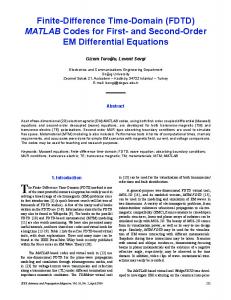
2 State of the art The classical FDTD method employs a second order finite centered approximation to the space and time derivatives in Maxwell’s curl equations, giving rise to to a new discrete electromagnetism with its own inherent peculiarities [8][9]. The FDTD defines an orthogonal cubic spatial grid whose unit cell is shown in figure 1; each field component is sampled and evaluated at a particular space position, and the magnetic and electric fields are obtained at time instants delayed by half the sampling time step. The materials are modeled by specifying their characteristic constants at every grid point, usually in homogeneous regions, at whose interfaces proper continuity conditions are needed. The time advancing algorithm is explicit, that is, the fields at each time instant are obtained as a function of previous values in time. The simulation of open problems is carried out by placing ABCs in the terminating planes of the grid. The method is fairly CPU and memory intensive, but current computing technology and foreseeable advances provide it with extraordinary power. Z EY

∆x

HZ EX

EX

∆z

EY

EZ

HY

EZ

EZ HX EY

EX

∆y Y

X

Figure 1: Yee unit cell

From the start, development of the original method has been aimed at enhancing its characteristics, either modifying the original algorithm, or using it in conjunction or hybridly with other techniques. Many papers have dealt with key aspects of the method and provided enhanced solutions (dispersion, material modeling, geometrical modeling, etc.), while others describe totally new concepts which provide the method with a new dimension (perfectly matched layer ABCs, unconditionally stable techniques, etc.). Some of the most interesting developments are described below. The error in the solution to a given problem depends on the algorithm employed to simulate each part of the problem, especially the discretisation of derivatives, geometrical and material modeling, and truncation conditions (ABCs). Second order approximation to derivatives implies a significant anisotropic phase error, although this may be negligible for electrically small problems. Nevertheless, today’s greater computing power allows us to deal with electrically large problems for which specific low–phase techniques should be employed. The most classical of these is the use of higher order approximations to derivatives [10], which reduces both dispersion and anisotropy, but many other FDTD–like techniques maintaining the marching–on–in–time scheme by using finite differences for the time derivatives, and using a different treatment for the spatial ones, are able to reduce the phase errors as well. For instance, the Pseudo Spectral Time Domain method (PSTD) [11] which obtains the space derivatives in the spectral space domain at each time step using the Fast Fourier Transform and its inverse (used in conjunction with the PML to prevent the wraparound effect). Another example is that of multiresolution techniques time domain techniques (MRTD) [12], which are also close to the FDTD method except that they obtain the spatial derivatives by means of scaling and wavelet functions. Currently promising lines of research aimed at low error schemes are based on the non–standard FDTD method (NS– FDTD) of Mickens [13] which is characterized by searching for zero truncation error (exact) schemes [14], or those based on the linear bicharacteristic schemes (LBS) [15]. On the other hand, the standard advancing algorithm is conditionally stable. The Courant criterion imposes an upper limit to the time increment related to the space increment employed in the discretisation. This can lead to high CPU times when a fine space discretisation implies the use of unnecessarily small time increments. New unconditionally stable techniques like the ADI–FDTD method [16][17], partially overcome the problem and have recently initiated an interesting research line. Although Mur absorbing boundary conditions [18] for open problems were the most commonly used for over a decade, the introduction of the Perfectly Matched Layer method by B´erenger in 1994 [19] represented a major advance in this field. Since then many publications have appeared in which they are studied, reformulated and enhanced. If the problem under simulation is periodic (for instance photonic bandgap, frequency selective surfaces, antenna arrays, etc.), specific boundary conditions (e.g. Floquet) are suitable to truncate it [20].

The discrete nature of the space time grid, and particularly the cubic staggered structure of Yee’s grid, introduce difficulties into the geometrical modeling of the materials, which lead to errors and even instabilities. Other geometrical aspects presenting difficulties are subcell details like wires, sheets, slots, edges and corners. Partial solutions are local or global finite integration/volume techniques [21][22], general curvilinear coordinates (orthogonal or not) [23], etc. all of which are attempts to conform the material geometry. Some simple variations of the homogeneous Yee grid (uneven meshes, subgridding) have also been proposed to help with this problem. A major concern with all these methods is their stability, for which the recently–announced unconditionally stable algorithms will probably provide solutions. A large part of the bibliography is devoted to seeking accurate solutions to these problems. Other studies carried out closely related to FDTD include: the near–to–far field conversion [3][24] mainly in the field of Radar Cross Section calculations, the simulation of sources internal or external to the computation domain, which may be lumped (for circuital structures) or wave source conditions (to simulate scattering problems) [25], etc. Finally, let us briefly mention the numerous efforts made to incorporate material behavior into the method, and the corresponding truncation conditions. Non– linear, dispersive, gyromagnetic, anisotropic, bi–isotropic, bi–anisotropic, active, metamaterial, random, periodic, photonic bandgap, are just some examples of the material structures that can be treated with the FDTD method. Numerous applications of the method have been published. One of the first was the calculation of the radar cross section (RCS) of arbitrary scatterers in the microwave range. Since then, the frequency range of the applications has grown to extend from low frequencies up to optical ones. The method has been used for circuit simulations, both lumped and distributed, and all kinds of waveguide propagation: conducting, dielectric, microstrip, coplanar, etc. It has been successfully used to simulate all kinds of antennas and arrays: wire, planar, microstrip, horn, etc. Its use in electromagnetic compatibility is also wide: shielding, coupling, natural or artificial (nuclear electromagnetic) pulse effects, etc. Its application to bioelectromagnetic problems such as hyperthermia, cancer detection, biological effects of electromagnetic waves, and specific absorption rate (SAR) calculations, is also a growing field of development, involving in many cases the coupling of Maxwell’s equations to heat and transport equations. Let us finish by summarizing some of the actual trends on FDTD methods. There is a constant inflow/outflow of new ideas with every other area involving the solution of partial differential equations: acoustic, computation fluid dynamics (CFD), quantum physics, etc. A common trend in all these disciplines is the search for more exact algorithms. The simulation of electrically large problems (like the ones in photonics) needs low dispersion error schemes. A desirable quality of any new numerical scheme is its unconditional stability so that the time discretisation can be chosen independently of the space discretisation, thus allowing them, for instance, to be applied to low frequency problems, or to problems meshed with structured or unstructured highly inhomogeneous grids, etc. The obtention of al-

gorithms, based on the integral or on the differential form, that are capable of characterizing the geometrical inhomogeneities of materials, continues to be a field of active research. Finally, there is growing interest in engineered materials which exhibit exotic electromagnetic properties, for which accurate simulation tools are needed. A great effort is to be dedicated to extend the new algorithms to deal with these materials.

3 Finite numerical schemes: an operational approach In this section we describe the fundamentals of the FDTD method. Since the following chapter deals with the implementation of free currents, we assume hence~ and magnetic J~ ∗ = forth that all the currents are ohmic, both electric J~ = σ E, ∗~ σ H (these last included for reasons of symmetry), with σ and σ ∗ being the electric and magnetic conductivity respectively. At this stage we also assume that all the ~ = εE, ~ B ~ = µH, ~ with ε and µ the media are linear, isotropic and non–dispersive D medium permittivity and permeability respectively, and so we omit the displacement and magnetic flux density vector fields, and set Maxwell’s curl equations in the so called E–H form, which in cartesian coordinates can be written as ~ + µ∂t H ~ , ∂˜r H ~ = σ E~ + ε∂t E~ −∂˜r E~ = σ ∗ H with



0  ∂˜r =  ∂z −∂y and in compact form as

 ∂y  −∂x  0

−∂z 0 ∂x

Ã

Ã

(4)

³ ´ ~ + S˜ψ ~ =R ~ ˜ ∂t ψ ˜ψ M ~ = (E, ~ H) ~ T , R ˜= ψ

S˜ =

(3)

σ I˜3 ˜03

˜03 σ ∗ I˜3

!

à ˜ = , M

(5)

˜03 −∂˜r

∂˜r ˜03

εI˜3 ˜03

˜03 µI˜3

!

! (6)

where henceforth I˜n , ˜0n denotes the n–th order identity and null matrices, respectively, and the superindex T the usual matrix transpose. To write the FDTD equations, let us first define the centered difference and average operators, δv f (v) =

f (v +

∆v 2 )

− f (v − ∆v

∆v 2 )

, av f (v) =

f (v +

∆v 2 )

+ f (v − 2

∆v 2 )

(7)

A Taylor series expansion proves that δv f (v) is a second order approximation to ∂v f (v), and av f (v) is a second order approximation to the identity opera˜ (v) = f (v). For instance, if f (v) is a one variable harmonic function tion If

f (v) = A cos(2π/λv v), the errors of the above defined operators with respect to the analytical ones are ¯ ¯ ¯ ∂v f (v) − δv f (v) ¯ π 2 1 ¯= εδ = ¯¯ ¯ ∂v f (v) 6 rv2

(8)

¯ ¯ ¯ f (v) − av f (v) ¯ ¯ ¯ = 3εδ εa = ¯ ¯ f (v)

(9)

λv with rv being the number of samples per oscillation in v (rv = ∆v ). Let us discretise the space into a set of points uniformly spaced in each direction, integer and semi–integer multiples of ∆x, ∆y, ∆z, and similarly the time into instants, integer and semi–integer multiples of a given interval ∆t, and let us define the fields at each spatial–temporal position of this grid with the following notation n ψi,j,k ≡ ψ(x = i∆x, y = j∆y, z = k∆z, t = n∆t)

(10)

The classical FDTD Yee numerical scheme is written, replacing the derivatives in (3) by the centered difference operator and averaging the conductivity terms in time n n n ~ i,j,k ~ i,j,k ~ i,j,k δ˜r H = σi,j,k at E + εi,j,k δt E n ∗ n n ~ i,j,k ~ i,j,k ~ i,j,k −δ˜r E = σi,j,k at E + µi,j,k δt H

(11)

where the numerical curl operator which approximates (4) is denoted by 

0  δ˜r =  δz −δy

−δz 0 δx

 δy  −δx  0

(12)

The heterogeneity of the media is handled by sampling the analytical constitutive parameters ε, µ, σ, σ ∗ at each point of the spatial grid εi,j,k ≡ ε(x = i∆x, y = i∆y, z = i∆z) . . .

(13)

Henceforth, cursive fonts are used for the numerical fields E, B, D, H, J to distinguish them from the analytical ones, for which a calligraphic font E, B, D, H, J is used. It can easily be appreciated that (11) does not involve all six components of the electromagnetic field, defined at every space point of the spatial grid sampled with ∆x/2, ∆y/2, ∆z/2. A grid six times less dense is enough with the fields relatively situated at the positions given by the Yee unit cell (figure 1). Similarly it is enough to define the electric fields at semi–integer multiples of the time increment ∆t

and the magnetic fields at integer multiples, to obtain the marching–on–in–time algorithm ∆t n ~ i,j,k ~ n+1/2 = εi,j,k − σi,j,k ∆t/2 E ~ n−1/2 + E δ˜r H i,j,k i,j,k εi,j,k + σi,j,k ∆t/2 εi,j,k + σi,j,k ∆t/2 ~ n+1 = H i,j,k

∗ µi,j,k − σi,j,k ∆t/2 n ∆t ~ ~ n+1/2 (14) H − δ˜r E i,j,k ∗ ∗ µi,j,k + σi,j,k ∆t/2 i,j,k µi,j,k + σi,j,k ∆t/2

with n integer, and i, j, k integer or semi–integer according to the position of the field component at the Yee cell. This algorithm is self–maintained, starting from numerical initial conditions sampled from the analytical ones. We can write (14) in compact form as ³ ´ ³ ´ ˜ i,j,k δt Ψ ~ n+1/2 + S˜i,j,k at Ψ ~ n+1/2 = R ˜Ψ ~ n+1/2 M i,j,k i,j,k i,j,k

(15)

with à n ~ ni,j,k = (E ~ n−1/2 , H ~ i,j,k ˜= Ψ )T , R i,j,k

à S˜i,j,k =

σi,j,k I˜3 ˜03

˜03 ∗ σi,j,k I˜3

!

˜03 −δ˜r Ã

˜ i,j,k = , M

δ˜r ˜03

!

εi,j,k I˜3 ˜03

˜03 µi,j,k I˜3

! (16)

which is formally similar to the analytic form (5) It is easy to build higher order schemes by using other approximations to the derivatives [26], which together with different collocations of the fields at the space grid, make it possible to manage, for instance, anisotropic media [27] with the E–H formulation. For instance, the operator ∆v 2 δ¯v ≡ δv − δv δv δv 24

(17)

is a fourth order approximation to the partial derivative with respect to v, with an error for a harmonic function εδ¯ = 2.7 ε2δ . The FDTD scheme has been successfully reformulated in other orthogonal coordinate systems, and even in general curvilinear coordinates [28][29]. It should be noted that, as later shown, although the E–H formulation is not well suited to deal systematically with arbitrary materials, it offers computational advantages over the material–independent D–B formulation for lossy media (isotropic or anisotropic) with no other dispersive characteristics. 1 1 A main advantage of the matricial operator language here introduced, and henceforth used in the whole chapter, is that is comprises a powerful and concise tool that furthermore permits the straightforward analysis, simplification, and construction of C/FORTRAN computer programs with the aid of the symbolic and code generation capabilities of tools like MathematicaT M

4 Fundamental topics: convergence, consistency, stability and dispersion An obvious quality of a good numerical scheme is that it should approximate the analytical equations when the space-time lattice is progressively refined ∆x, ∆y, ∆z, ∆t → 0. Such a scheme is said to be consistent with the analytical problem. If we define the n local truncation error of a given numerical scheme written in o n ˜ ~ the generic form L Ψi,j,k = 0, as n o n ~n ˜ ψ T~i,j,k =L i,j,k

(18)

~ n the ana~ n representing the solution of the numerical scheme and ψ with Ψ i,j,k i,j,k lytical solution sampled at (x, y, z, t) = (i∆x, j∆y, k∆z, n∆t), we can formally say that the scheme is consistent if [30] lim

∆x,∆y,∆z,∆t→0

n T~i,j,k =0

For instance, for eqn. (15) the local truncation error is ³ ´ n ~ n+1/2 ˜ i,j,k δt + S˜i,j,k at − R ˜ ψ = M T~i,j,k i,j,k

(19)

(20)

~ n is the analytical field where ψ i,j,k ~n = ψ i,j,k

µ ¶T 1 ~ ~ E(i∆x, j∆y, k∆z, (n − )∆t), H(i∆x, j∆y, k∆z, n∆t) (21) 2

sampled at lattice space and time positions. A multidimensional Taylor series leads us to n ~ n00 0 0 , n ≤ n0 ≤ n + 1 T~i,j,k = F˜ (∆x2 ∂x3 , ∆y 2 ∂y3 , ∆z 2 ∂z3 , ∆t2 ∂t3 )ψ i ,j ,k

i−

1 1 1 1 1 1 ≤ i0 ≤ i + , j − ≤ j 0 ≤ j + , k − ≤ k 0 ≤ k + 2 2 2 2 2 2

(22)

with F˜ being a matrix operator involving a linear combination of its arguments. Thus, the Yee scheme is unconditionally consistent with Maxwell’s curl equations up to second order, with truncation error terms in (22) written in the frequency and spectral–space domain as ∆α2 ∂α2 → 1/rα2 with rα being the number of samples per oscillation (α = {x, y, z, t}). The consistency of a numerical scheme, in any case, does not guarantee that its solution actually approximates the analytical solution. A numerical scheme is said to be convergent [30][31] if its solution tends to the analytical one when the spacetime lattice is progressively refined at a given space–time point (x = i∆x, y = j∆y,z = k∆z,t = n∆t), that is, when ∆x, ∆y, ∆z, ∆t → 0, and i, j, k, n → ∞.

Finally, for a well–posed analytical initial value problem, given a numerical scheme replacing it, the difference of the numerical solutions for arbitrarily bounded differences in the initial values must be bounded in the same manner, as are the analytical ones. Such a scheme is said to be stable. If the solution of the analytical initial value problem is naturally bounded in time (for instance, Maxwell’s curl equations for passive media), then any stable scheme replacing it must necessarily keep its solution bounded in time as well. The Lax equivalence theorem [31] states that given a well–posed initial-value problem and a consistent linear finite-difference numerical scheme, stability is the necessary and sufficient condition for convergence. The utility of this theorem is obvious since it is usually easier to find stability criteria rather than convergence ones, and we need only to guarantee then stability of a consistent scheme to conclude that the numerical solution actually approximates the right solution. 4.1 Dispersion relation: Von-Neumann stability criterion Plane waves propagating in lossless non–dispersive isotropic linear homogeneous media have a phase speed independent of the frequency and the propagation direction. Let us study how the numerical scheme propagates such plane waves. We can write the Yee scheme (15) for such media as n+1/2

~ δt Ψ i,j,k

˜ ˜T Ψ ~ n+1/2 , R ˜ T = (M ˜ i,j,k )−1 R = R i,j,k

(23)

with known initial values that can be expanded in Fourier series in generic terms ~ 0 e j (−i∆x βx −j∆y βy −k ∆z βz ) Ψ

(24)

with β~ = (βx , βy , βz ) the real wavevector. Let us assume that this harmonic, which is analytically propagated¡ harmonically ¢in time with frequency fulfilling the dispersion relation µεω 2 = βx2 + βy2 + βz2 , is also propagated harmonically by the scheme with a complex frequency Ω ~ ni,j,k = Ψ ~ 0 e j (n∆t Ω−i∆x βx −j∆y βy −k ∆z βz ) Ψ

(25)

Inserting (25) into the numerical scheme (23) the following eigen–value problem is obtained ³ ´ ˜R Ψ ~ n+1/2 = 0 Λt I˜6 − Λ (26) T

i,j,k

with à ˜R = Λ T

˜06 ˜δ −1/µ Λ r

˜δ 1/ε Λ r 0˜6

!



0

˜δ =  , Λ  Λz r −Λy

−Λz 0 Λx

Λy



 −Λx  0

µ ¶ µ ¶ 2j ∆t 2j ∆α Λt = sin Ω , Λα = sin βα , α = {x, y, z} ∆t 2 ∆α 2

(27)

Imposing a non trivial solution (null determinant of the coefficient matrix), leads to √ c−2 Λ2t = Λ2x + Λ2y + Λ2z , c = 1/ εµ (28) Explicitly µ ¶ ∆t 1 2 sin Ω = c2 ∆t2 2 µ ¶ µ ¶ µ ¶ 1 1 1 ∆x ∆y ∆z 2 2 2 sin βx + sin βy + sin βz ∆x2 2 ∆y 2 2 ∆z 2 2

(29)

which is seen to approximate the analytic dispersion relation in the limit of null increments. The phase speed vf = Ω β is shown to depend both on frequency (dispersivity), and on the propagation direction (anisotropy) unlike the analytical phase speed (see [4] for further details). Furthermore the structure relationship between the direction of propagation, the electric field and the magnetic field (orthogonal in the analytic case) is no longer valid. By extracting the time eigen–value from (28) and introducing it into (26) we obtain for the amplitudes 1 ~ ~n · E ~0 , β ~0 = 0 βn × E (30) µ Ωn µ ¶ sin (βx ∆x/2) sin (βy ∆y/2) sin (βy ∆y/2) sin (Ω∆t/2) ~ βn = , , , Ωn = ∆x/2 ∆y/2 ∆z/2 ∆t/2 (31) where it can be seen that the electric field and the magnetic field are mutually perpendicular; however they are not perpendicular to the analytical wavevector ~ = (βx , βy , βz ) but to a numerical–like wave-vector defined by (31). β As previously stated, a necessary condition of stability is that the solution of the scheme must remain bounded in time; in this case ¯ ¯ ¯ jΩ∆t ¯ (32) ¯e ¯ ≤ 1 ⇔ Im {Ω} ≥ 0 ~0 = H

~ if From (29), condition (32) holds ∀β s µ µ µ ¶ ¶ ¶ ∆x ∆y ∆z 1 1 1 2 2 2 sin βx + sin βy + sin βz ≤1 c∆t ∆x2 2 ∆y 2 2 ∆z 2 2 (33) which always holds if the Courant number s next defined fulfills r 1 1 1 s ≡ c∆t + + ≤1 (34) 2 2 ∆x ∆y ∆z 2

¯ ¯ ¯ ¯ which implies Im {Ω} = 0 and ¯e jΩ∆t ¯ = 1. When ∆x = ∆y = ∆z ≡ ∆, the √ condition on the Courant number becomes s = 3 c∆t ∆ ≤ 1. This condition, properly known as the Von–Neumann stability criterion, coincides with the CourantFriedrichs-Lewy (CFL) condition (also known as the causality condition) obtained through geometrical considerations on the characteristics of the hyperbolic differential system [30]. We can conclude that there is an upper limit to choose the time increment, after the space increments are chosen, which may lead to unnecessarily small increments for certain problems. If the necessary condition (34) does not hold, there appear both increasing solutions (unstable) and decreasing ones (dissipative) propagating at the Nyquist frequency If sin(Ω

³ ´ p ∆t π 2 )=g>1 ⇒ Ω= ± j ln g + g 2 − 1 2 ∆t ∆t

(35)

It can be demonstrated that condition (32) is also sufficient for the homogeneous initial value problem. Nevertheless, in the presence of inhomogeneities (material changes, space increments depending on the space position, boundary conditions, etc.), or, in general, when the problem becomes an initial boundary value problem (any computational implementation must necessarily incorporate boundary conditions), condition (32) may not be sufficient but only necessary to guarantee stability. In these cases we can use the Gustaffson-Kreiss-Sundstrom theory [32] ¯ ¯ ¯ ¯ which pays special attention to the critical case ¯e jΩ∆t ¯ = 1, showing that there can appear instabilities depending on the specific boundary conditions (see [33] for a physical reinterpretation of this theory in terms of group speed). 4.2 Spectral stability criteria It is possible to find an analytic formulation based on spectral analysis permitting us to investigate, at least numerically, the stability of problems solved in a closed region with appropriate boundary conditions (initial boundary value problems). Let us state the two–level scheme (23) expressed by ~ n+1 = Ψ ~ ni,j,k + ∆tR ˜T Ψ ~ n+1/2 Ψ i,j,k i,j,k

(36)

as a single–level scheme ! Ã n+1/2 ! ! Ã ˜ T I˜6 ~ n+1 ~ ∆t R Ψ Ψ i,j,k i,j,k ~ n+1 = G ˜Φ ~ n+1/2 = ⇒Φ n+1/2 i,j,k i,j,k ˜6 ~ ~n ˜06 I Ψ Ψ i,j,k i,j,k | {z } | {z }| {z } Ã

˜ G

~ n+1 Φ i,j,k

~ n+1/2 Φ i,j,k

(37) holding for every point inside the closed region, plus the specific conditions at the n o ~n ~ n defined boundaries F˜ Φ = 0. It is possible to reorder the unknowns Φ i,j,k i,j,k B

at all the positions of the three–dimensional space grid into a one–dimensional ~ n and so (37) can be rewritten as column matrix Φ ~ n+1 = G ˜Φ ~ n+1/2 + ~b n+1/2 Φ

(38)

˜ being the scheme amplification matrix and ~bn the column matrix with the with G boundary conditions. It can be proven that a necessary condition for stability is that ˜ ≤ 1. The result is the spectral radius of the amplification matrix must fulfil ρ(G) ~ 0 are propagated clearly justified because (38) implies that the initial conditions Φ by increasing powers of the amplification matrix. ³ ´2(n+1) 0 ~ n+1 ∼ G ˜ ~ Φ Φ

(39)

and the spectral radius is a lower bound of any compatible matrix norm [31]. Although this criterion may seem difficult to put into practice, since it is cumbersome to find the spectral radius for a given symbolic problem analytically, it can be systematically applied to particular numerical benchmark cases because the sparse nature of the amplification matrix allows us to use rapid routines (for instance LAPACK) to obtain its spectral radius. The main utility of this technique is to test inhomogeneous schemes for instabilities (uneven meshes, subgridding, locally distorted conformal schemes, etc.) where the Von–Neumann technique is not applicable.

5 Truncation conditions: Perfectly Matched Layer (PML) The FDTD method permits the solution of open problems in computationally bounded domains by employing suitable truncation conditions. These simulate a frontier which ideally is transparent (null reflection coefficient) irrespective of the frequency, polarization and angle of incidence. The Mur absorbing boundary conditions [18] for open problems were the most commonly used for more than a decade. Although they offered reflection coefficients of up to -40 dB, this was not enough for many interesting problems. Many alternatives have been developed since then [34] to reduce the reflection coefficient up to -100 dB. But in 1994 B´erenger with his Perfectly Matched Layer method [19] provided a non Maxwellian analytic technique achieving up to -140 dB. Its main characteristic was its ease of implementation in working FDTD codes, and its apparent simplicity. Further works to obtain PML Maxwellian formulations has since been carried out [35][36], and are briefly described at the end of this section. The fundamental idea of the original PML technique is the truncation of one Maxwellian medium, by means of a non Maxwellian one, which is perfectly absorbing for all frequencies, polarizations and angles of incidence, and able to totally attenuate, from a practical point of view, the field propagated in its interior, after the propagation of just a few cells. This absorbing layer can then be terminated by a perfect electrically/magnetically conducting (PEC/PMC) wall, so that

it can be implemented without requiring high computational resources. Although such a medium is theoretically unphysical, it is possible to build a mathematical set of Maxwell–like equations on which to enforce such conditions. Initially the term PML was related only to the work of B´erenger, but it has since become a common term for the set of techniques, based or not on B´erenger’s initial equations, with the common characteristic of being able to truncate the computational space by an absorbing transparent layer. B´erenger’s main idea was to construct an electric and a magnetic pseudo–field, by splitting each cartesian component of the Maxwellian field into two subcomponents, and relating each time derivative of them with only one part of the spatial derivatives appearing in the curl equation of the Maxwellian component, so that the addition of the equations fulfilled by both subcomponents would recover the original curl equation. By now introducing into the equation of each subcomponent the possibility of anisotropic electric and magnetic conductivities, a new set of equations is obtained, with enough degrees of freedom to achieve the objective that every solution of Maxwell’s curl equations should also be a solution of B´erenger’s equations on an arbitrary surface separating the solution domains of each set of equations (continuity of both solutions). Thus any wave propagating in the Maxwellian medium will be transmitted into the B´erenger domain without reflection, where it will propagate with attenuation due to the conductivity terms. Although this interpretation of B´erenger’s PML, which we will develop below, differs from the original one [19], we find it very general and relatively simple to understand. Let us assume a source–free medium inside which there are plane waves propagating with the form ~ r) ~ r, t) = ψ ~0 e j (ω t−β·~ ψ(~ (40) ~ related by the medium dispersion relation, for which Maxwell’s curl with ω and β equations expressed in material–independent form are ~ , −j β˜H ~ = j ωD ~ j β˜E~ = j ω B with



0  β˜ =  βz −βy

−βz 0 βx

 βy  −βx  0

(41)

(42)

representing the curl–like wavenumber matrix. And let us assume a general relationship between the fields in the frequency domain ~ = ε˜(ω) E~ , B ~=µ ~ D ˜(ω) H

(43)

with ε˜(ω), µ ˜(ω) already including the electric and magnetic conductivity losses and dispersivity, as well as anisotropy.

Let us assume that we truncate this Maxwellian medium by another one, henceforth called PML, in which we define a pseudo–field splitting each field cartesian ¡ ¢ ~ PML = ψ PML , ψ PML , ψ PML T into two subcomponents component ψ x y z ~ PML = (ψ PML , ψ PML , ψ PML , ψ PML , ψ PML , ψ PML )T , ψ = {E, H, D, B} ψ s xy xz yz yx zx zy | {z } | {z } | {z } PML ψx

ψyPML

(44)

ψzPML

which recover the original three–component field when added   1 1 0 0 0 0  ~ PML = C˜ ψ ~ PML , C˜ =  ψ  0 0 1 1 0 0  s 0 0 0 0 1 1

(45)

Let us force the split field to fulfil equations somehow similar to (41) but including anisotropic lossy terms through conductivity matrices σ ˜s and σ ˜s∗ ~sPML , − j˜ ~ sPML = jω D ~ sPML + σ ~ sPML ~sPML + σ γs C˜ H ˜s D j˜ γs C˜ E~sPML = jω B ˜s∗ B with γ˜s a split curl–like wavenumber matrix  0 0   0 −γ z   γ 0  z γ˜s =   0 0   0 γx  −γy 0

γy 0 0 −γx 0 0

(46)

          

(47)

and with general frequency domain constitutive relationships of the form ~ sPML = ε˜s (ω)E~PML , B ~sPML = µ ~ sPML D ˜s (ω)H

(48)

Eqn. (46) is satisfied by plane waves of the form ~s (~r, t) = ψ ~s0 e j (ω t−~γ ·~r) ψ

(49)

with ω and γ related by the PML dispersion relation. If a plane wave (40) propagating inside the original medium is incident on a plane interface with the PML medium and a transmitted wave (49) begins to propagate inside it, no reflection will occur at the interface, whatever the angle of incidence, frequency and polarization, if there is continuity of all the components of the fields in the original medium with those of the compact field in the PML. For instance for the interface plane x = 0 ´ ´ ³ ´ ³ ´ ³ ³ ~=B ~ PML ~ =D ~ PML ~ =H ~ PML , B , D , H E~ = E~PML x=0

x=0

These continuity conditions imply

x=0

x=0

(50)

³ ´ ~ • Phase continuity e j β~r = e j ~γ ·~r ⇒ γy = βy , γz = βz with γx x=0 arbitrarily chosen ~0 = D ~ PML , B ~0 = B ~ PML , E~0 = E~PML , H ~0 = • Amplitude continuity D 0 0 0 PML ~ H0 ˜s , ε˜s , µ ˜s to ε˜, µ ˜ for this to Let us obtain the relationship that must relate σ ˜s∗ , σ PML ~ and D ~ from (41) and B ~s and D ~ sPML from (46) and using (45), occur. Extracting B the amplitude continuity is fulfilled if 

σy 0 0 0

     ∗ σ ˜s = σ ˜s =     0  0

0 σz 0 0

0 0 σz 0

0 0 0 σx

0 0 0 0

0 0

0 0

0 0

σx 0

0 0 0 0



      ,   0   σy

³ σα ≡ jω

γα βα

´ −1

α = {x, y, z}

(51)

and C˜ ε˜s (ω) = ε˜(ω) C˜ , C˜ µ ˜s (ω) = µ ˜(ω)C˜

(52)

On the other hand, the phase continuity condition at x = 0 implies γy = βy , γz = βz with which σy = σz = 0, freeing the choice of γx which can be taken as γx = βx − jκx with κx an arbitrarily real coefficient which controls the attenuation rate inside the PML. For this choice σx = βωx κx is a real number. Fixing this conductivity for a given problem, the attenuation rate κx will be frequency independent for frequency independent media (ω/βx = vx with vx phase speed). Nevertheless, for dispersive media it is necessary to use an optimum conductivity value to obtain the desired attenuation rate for the worst frequency case. Finally, the wave propagating into the PML takes the form σ

~s (~r, t) = ψ ~s0 e j (ω t−γx x−βy y−βz z) = ψ ~s0 e j (ω t−βx x−βy y−βz z) e− vxx x ψ

(53)

It could even be possible to add extra degrees of freedom to (46), also permitting the absorption of evanescent waves [37][38], although we will refer later to more recent approaches. Hence, the time domain PML equations matching the Maxwell’s curl equations ~ , ∂˜r H ~ = ∂t D ~ −∂˜r E~ = ∂t B

(54)

are ~sPML + σ ~sPML , ∂˜rs C˜ H ~ sPML = ∂t D ~ sPML + σ ~ sPML −∂˜rs C˜ E~sPML = ∂t B ˜s B ˜s D

(55)

with



∂˜rs

     =    

0 0 ∂z 0 0 −∂y

0 −∂z 0 0 ∂x 0

∂y 0 0 −∂x 0 0

          

(56)

and with the constitutive relationship time domain versions of (43) and (48) taking into account (52), which for non–dispersive lossless isotropic media is fulfilled by ε˜(ω) = εI˜6 and µ ˜(ω) = µI˜6 . For this last sort of media, and even for anisotropic ones, an E–H formulation could be used for computational efficiency, which would be totally equivalent to the material–independent form here described [39][40]. Nevertheless the material–independent form shows its generality for dispersive media. For instance, for a Debye dielectric dispersive isotropic non-magnetic medium µ ¶ εs − ε∞ σ ˜ ε˜ = ε∞ + I3 , µ ˜ = µ0 I˜3 (57) + 1 + jωτ jω (43) can be written in the time domain in partial differential equation form (jω → ∂t ) ~ = µ0 H ~ ~ + ∂t D ~ = τ ε∞ ∂t2 E~ + (εs + τ σ) ∂t E~ + σ E~ , B (58) τ ∂t2 D and (48) in a formally identical way ~ sPML = τ ε∞ ∂t2 E~sPML + (εs + τ σ) ∂t E~sPML + σ E~sPML ~ sPML + ∂t D τ ∂t2 D ~ sPML ~sPML = µ0 H B since

µ ¶ εs − ε∞ σ ˜ ε˜s = ε∞ + I6 , µ ˜s = µ0 I˜6 + 1 + jωτ jω

(59)

(60)

satisfies the condition (52). A number of extensions to all kinds of media can be performed (for instance, in [41] a PML to adapt bianisotropic media is obtained) with the same construction principles followed here, i.e., imposing total continuity on the fields at the interface between the two media. Although we could add extra degrees of freedom to the above equations to extend the capabilities of the method, it is easier, for many cases of interest, to handle its extension via a previous Maxwellian reformulation. An equivalent Maxwellian reformulation of the method can readily be obtained ˜ and taking into acby left–multiplying eqn. (55) in the frequency domain by C, count (45) " µ # ¶−1 1 ˜ ˜ ˜ ~ PML σ ˜s − C I6 + ∂rs E~PML = jω B jω

" µ # ¶−1 1 ~ PML = jω D ~ PML C˜ I˜6 + σ ˜s ∂˜rs H jω which after defining a set of stretched spatial variables of the form Z α σα α0 = , α = {x, y, z} sα (ξ)dξ ⇒ ∂α = sα ∂α0 with sα = 1 + jω 0

(61)

(62)

can be written as ~ PML , ∂˜r0 H ~ PML = jω D ~ PML −∂˜r0 E~PML = jω B

(63)

with ∂˜r0 being the usual curl operator (4) with derivatives with respect to the stretched spatial variables. We can re–scale each cartesian component of the fields according to ψα0 = ψα sα , ψ = {E, H, D, B} , α = {x, y, z}

(64)

and alternatively write 0 ~ PML0 , ∂˜r H ~ PML0 = jω˜ ~ PML0 −∂˜r E~PML = jω s˜B sD

with

  s˜ = 

sy sz sx

0 0

0 sz sx sy

0

0 0 sx sy sz

(65)

   , sα = 1 +

1 jωσα

(66)

Relation (65) together with (66) is the uniaxial formulation of the perfectly matched layer (UPML). Notice that both the stretching technique [35][42] and the UPML [36][43] are equivalent in their absorption capabilities to the split B´erenger PML [44]. The stretched variable formulation has proven to be useful to extend the method to non cartesian coordinates [45], to absorb efficiently both propagative and evanescent waves (complex frequency-shifted (CFS)-PML) [46][47], to absorb waves in bianisotropic lossy media [48], etc. A drawback of the split equation resides in the fact that it actually supports not only plane waves with frequency and wavenumber related by the dispersion relation, but also a subcomponent of the field can be increasing, while the other one decreases, linearly in time, as proven in [49], exactly cancelling out this behavior when the two subcomponents are added. This may lead to late time instabilities associated with round–off errors as seen in [50]. In relation to the implementation of the split B´erenger’s PML time domain equations (55) it is straightforward to obtain an explicit finite difference numerical scheme in a similar way to that employed with Maxwell’s time domain equations: namely replacing all the derivatives by their finite centered approximation and averaging in time all the fields affected by conductivity terms in eqn. (55), placed at

the space positions given by the Yee cube, and at time instants delayed by half the time increment between the electric and magnetic fields. The time domain electric constitutive relationship must be advanced after advancing the displacement field and before advancing the magnetic field, and the time domain magnetic one, after the latter and before closing the loop (see the section on material modeling for more details). The particular implementation in the time domain of the UPML and of the stretching technique depends on the specific form of the sα . For instance, for the (CFS)-PML, the causal form [47] sα = κ α +

σα ηα + jωχα

(67)

which is suitable to absorb evanescent waves, can be efficiently implemented in a recursive convolutional form [46]. A common characteristic of these methods is that the conductivity profile inside the PML is implemented numerically as an increasing function, so that the attenuated transmitted wave can be numerically negligible in less than 12 cells of propagation. Typically the conductivity is increased in a polynomial profile of order between 2 and 4 to obtain a theoretical normal attenuation around -120 dB µ σα =

σαmax

ρα dα

¶n (68)

with the notation of figure (2). Since the PML is truncated with PEC or PMC conditions, the calculated refflection coefficient as a function of the incidence angle θ is 2

r(θ) = e− n+1

max σα vα

dα cos θ

(69)

where for anisotropic media and/or dispersive media it should be taken into account that the phase speed can depend on the propagation angle and/or frequency of the waves. Finally, using the same construction, it can be seen that at the interface of two PML media with given conductivities, perfect matching with attenuation is achieved if equal conductivity terms corresponding to the plane interface directions are chosen. This is useful to determine which conductivity terms must be used at the edges and corners of the computational domain. For instance, in figure (2) the 2D corner region has the same σy as the left PML region, with no restriction on σx , and, reciprocally, it has the same σx as the upper PML region, with no restriction on σy . The result is a region with two non–null conductivities.

PEC

 





























 














PEC













































 











 

















 
  
  
  
  
  
  
  
  
  
  
  
  
 
 
 
 
 
 
 

           







 


                                      
 






                                             









          σ x=σ     x                           
 σ
x
       x=σ








 1 







           σ  =   0  1                          





 σ
 y=σ 
 y2


             y                              


















                               ρ x           

 

       
















   
















 
 

         

      






 
 
      






 
      






  
 
















 

       

         






  
















 
 

       
 

      






  
 

 =










σ 0
 
      
x

        







  
















 
 

       
σ =σ  

      






  
y y 













2
 
       
 
        







  Ε 
















 
 

       
β  

       






  















 








 
 

       
 

      






  θ 















 
       
 
        







  
















 
 

       
 

      






  














 
       
ρ

         







  















y

 

        

      






 
 







 
 
 
 
 
 
 
  

X

Y

dx

dy Figure 2: Conductivity implementation at a 2D PML corner

6 UNCONDITIONALLY STABLE METHODS: ADI-FDTD There is increasing interest in the design of unconditionally stable algorithms as an alternative to the Yee one. Several starting points are possible: operational approaches [51], brute–force Crank–Nicolson methods [52], implicit lower-upper approximate factorization (LU/AF) [53], Alternating Direction Implicit (ADI) split– step methods [16][17], etc. The latter, known as ADI–FDTD, has inspired this new line of research, and is described in detail in this section. In the traditional explicit Yee FDTD algorithm, the time increment cannot exceed the Courant stability limit, and therefore the maximum time-step size is restrained by the smallest spatial increment in the computational domain. This means that when a fine mesh is needed to model part of the computational domain (for instance by subgridding or uneven mesh techniques), the Courant condition results in an oversampling in time, which leads to high computation times. An alternative to the standard explicit FDTD method, the Alternating Direction Implicit Finite Difference Time Domain (ADI-FDTD) method, has been proposed

in [16][17]. The ADI is a technique first found in the works of Peaceman, Rachford and Douglas [54][55] used to perturb and factorize the unconditionally stable Crank–Nicolson scheme approximation of partial differential equations, to render it computationally costless without losing its unconditional stability. For Maxwell’s curl equations, the ADI–FDTD is based on an implicit-in-space formulation of the FDTD, which offers unconditional numerical stability with little extra computational effort. The ADI-FDTD method removes the stability limit for the time increment, making it possible to choose the time increment independently of the space increment. Thus, this technique allows us to choose dense spatial grids where needed without necessarily requiring the use of small time increments. Since the ADI-FDTD method keeps the Yee spatial distribution of the fields, it can be applied to the whole range of problems addressed by the original Yee method. Nevertheless, the time increment cannot be increased arbitrarily taking into account only numerical dispersion criteria (number of samples per period); it is also limited by the fact that it must accurately resolve the spatial variations of the fields [56] as we will see later. In spite of this, in many practical problems the method still achieves significant reductions in CPU time compared to the FDTD method. Let us start by building a Crank–Nicolson FDTD (CN–FDTD) scheme by averaging in time the right hand side of (15) ³ ´ ³ ´ ³ ´ ˜ i,j,k δt Ψ ~ n+1/2 + S˜i,j,k at Ψ ~ n+1/2 = R ˜ at Ψ ~ n+1/2 M (70) i,j,k i,j,k i,j,k ~ n = (E ~n ,H ~ n ), which after defining now with Ψ i,j,k i,j,k i,j,k à σi,j,k ³ ´−1 ³ ´ − εi,j,k I˜3 ˜ ˜ ˜ ˜ RT = Mi,j,k R − Si,j,k = 1 ˜ − µi,j,k δr

1 ˜ εi,j,k δr σ∗ − µi,j,k I˜3 i,j,k

! (71)

leads us to

³ ´ ~ n+1 − Ψ ~ ni,j,k = ∆t R ˜T Ψ ~ n+1 + Ψ ~ ni,j,k Ψ (72) i,j,k i,j,k 2 The application of the CN-FDTD scheme (72) to practical problems requires prohibitively large computational resources [52], since it involves the solution of a sparse linear system of equations at each time step. Using the ideas of Peaceman, Rachford and Douglas [54] [55] it is possible to factorize the CN–FDTD scheme into a two-sub–step procedure, each one only needing the solution of a tridiagonal system of equations, by adding a second order perturbation term in the following manner ³ ´ µ ∆t ¶2 ³ ´ ³ ´ n+1 n ~ ~ ˜T Ψ ~ n+1 + Ψ ~ ni,j,k ˜ Ψ ~ n+1 − Ψ ~ ni,j,k = ∆t R Ψi,j,k − Ψi,j,k + A˜B i,j,k i,j,k 2 2 {z } | P erturbation

˜ are chosen so that If the operators A˜ and B ˜=R ˜T A˜ + B

(73) (74)

(73) can be rewritten as µ ¶µ ¶ µ ¶µ ¶ ∆t ˜ ∆t ˜ ~ n+1 ∆t ˜ ∆t ˜ ~ n I˜6 − A I˜6 − B Ψi,j,k = I˜6 + A I˜6 + B Ψi,j,k (75) 2 2 2 2 and factorized into a two-sub-step procedure as µ ¶ µ ¶ ∆t ˜ ~ n∗ ∆t ˜ ~ n I˜6 − A Ψi,j,k = I˜6 + B Ψi,j,k 2 2 µ ¶ µ ¶ ∆t ˜ ~ n∗ ∆t ˜ ~ n+1 I˜6 − B Ψi,j,k = I˜6 + A Ψi,j,k 2 2 ~ n∗ being an auxiliary intermediate vector field. with Ψ i,j,k ˜ which fulfills (74), is A convenient choice of A˜ and B, à ! à σ σ 1 ˜ − 2 εi,j,k − 2 εi,j,k I˜3 I˜3 εi,j,k δre i,j,k i,j,k ˜ ˜ ∗ A= , B = σ 1 ˜ 1 ˜ δro − 2 µi,j,k I˜3 δre − µi,j,k − µi,j,k i,j,k 

0  δ˜re =  δz 0

0 0 δx

with which we can write à !à l1 I˜3 −l2 δ˜re l3 δ˜ro l4 I˜3 à !à l1 I˜3 −l2 δ˜ro l3 δ˜re l4 I˜3





δy 0   0  , δ˜ro =  0 0 −δy ~ n∗ E i,j,k ~ n∗ H i,j,k ~ n+1 E i,j,k ~ n+1 H i,j,k

!

à =

!

à =

−δz 0 0

l5 I˜3 −l3 δ˜re

l2 δ˜ro l6 I˜3

l5 I˜3 −l3 δ˜ro

l2 δ˜re l6 I˜3

(76) (77)

1 ˜ εi,j,k δro ∗ σi,j,k − 2 µi,j,k I˜3

(78)



0  −δx  0 !Ã

!Ã

~n E i,j,k ~n H i,j,k ~ n∗ E i,j,k ~ n∗ H i,j,k

!

(79)

!

! (80)

defining l1 = 1 + l4 = 1 +

∆t σi,j,k ∆t 4 εi,j,k , l2 = 2 εi,j,k ∗ ∆t σi,j,k ∆t 4 µi,j,k , l3 = 2 µi,j,k

, l5 = 1 − , l6 = 1 −

∆t σi,j,k 4 εi,j,k ∗ ∆t σi,j,k 4 µi,j,k

(81)

In order to solve the system of equations (76) and (77) explicitly in time for ~ n∗ and H ~ n∗ we first put it in triangular form E i,j,k i,j,k à !à ! ~ n∗ l4 l1 I˜3 + l3 l2 δ˜re δ˜ro ˜03 E i,j,k = ~ n∗ l3 δ˜ro l4 I˜3 H i,j,k ³ ´ !à à ! ~n l4 l5 I˜3 − l3 l2 δ˜re δ˜re l2 l6 δ˜re + l4 δ˜ro E i,j,k ~n H −l3 δ˜re l6 I˜3 i,j,k ! à !à ~ n+1 l4 l1 I˜3 + l3 l2 δ˜ro δ˜re ˜03 E i,j,k = ~ n+1 H l3 δ˜re l4 I˜3 i,j,k

Ã

l4 l5 I˜3 − l3 l2 δ˜ro δ˜ro −l3 δ˜ro

´ !Ã ³ ! ~ n∗ l2 l4 δ˜re + l6 δ˜ro E i,j,k ~ n∗ H l6 I˜3 i,j,k

(82)

This system of equations can now be solved by back–substitution at each time ~ n∗ , then H ~ n∗ , and similarly to advance step: to advance from n to n∗ , first obtain E ∗ from n to n + 1. It can be seen that at each sub–step n∗ and n + 1 only the electric field equations involve the solution of a system of equations which is tridiagonally implicit–in–space because the operators δ˜ro δ˜re and δ˜re δ˜ro only use second order differences in one direction in turn. 

0 δx δy 0  ˜ ˜ δre δre =  0 0 δy δz δz δx 0 0  2 δz 0 0  ˜ ˜ δro δre = −  0 δx2 0 0 0 δy2

     



0  ˜ ˜ , δro δro =  δx δy 0  2 δy  ˜ ˜ , δre δro = −  0 0

 δz δx  0  0 

0 0 δy δz 0 δz2 0

0  0  δx2

(83)

The magnetic field is obtained explicitly in space. In the lossless case (σ = σ ∗ = 0), eqns. (82) coincide with the usual algorithm described in [16][17] in n∗ = n + 12 . Ã

Ã

I˜3 − Ã

Ã

I˜3 −

I˜3 +

∆t2 ˜ ˜ 16εi,j,k µi,j,k δre δro ∆t ˜ 2 µi,j,k δro

∆t2 ˜ ˜ 16εi,j,k µi,j,k δre δre − 2 µ∆t δ˜re i,j,k

I˜3 +

∆t ˜ 2 εi,j,k R

!Ã

˜03 I˜3

∆t ˜ 2 εi,j,k R

~ n∗ E i,j,k ~ n∗ H

! =

i,j,k

!Ã

I˜3

∆t2 ˜ ˜ 16εi,j,k µi,j,k δro δre ∆t ˜ 2 µi,j,k δre

∆t2 ˜ ˜ 16εi,j,k µi,j,k δro δro δ˜ro − 2 µ∆t i,j,k

˜03 I˜3

!Ã

!Ã

I˜3

~n E i,j,k ~n H i,j,k ~ n+1 E i,j,k ~ n+1 H i,j,k

~ n∗ E i,j,k ~ n∗ H i,j,k

!

! = ! (84)

PML absorbing boundary conditions have been obtained for the ADI-FDTD method both in the B´erenger split form [57] and in the stretched coordinate metric [58]. An interesting alternative approach to build unconditionally stable schemes can ~ be a normalized field vector be found in [51]; let us summarize it briefly. Let ψ ~= ψ

³√

~ ε E,

√ ~ ´T µH

(85)

so that Maxwell’s curl equations are written (in the lossless current–free case for simplicity) Ã

˜03 1 − √ δ˜r √1

~ ~ ˜ N ψ(t) ˜N = ∂t ψ(t) =R , R

µ

˜ √1 √1 δ ε r µ

ε

˜03

! (86)

~ With this normalisation, the usual spatial euclidean L2 –norm of the vector ψ gives a measure of the electromagetic energy. The formal solution of (86) with ~0 , is formally initial conditions in time ψ ~ = et R˜ N ψ ~0 ψ

(87)

where the absence of currents implies that the total energy is conserved (the L2 – ~ coincides with that of ψ ~0 ). Hence the time operator et R˜ N is orthogonal; norm of ψ ~0 to obtain ψ ~ from it. Thus a semidiscrete time it merely rotates the initial state ψ advancing scheme of the form ~n ~ n+1 = e∆t R˜ N ψ Ψ

(88)

becomes straightforwardly stable. ˜ Any orthogonal spatial approximation to et RN will also be necessarily stable in time. A useful one is given by the Lie-Trotter-Suzuki formula [59] to approximate matrix exponentials t

e

p P i=1

Ã

˜i H

= lim

m→∞

p Y

!m ˜ i /m tH

e

(89)

i=1

whose first order approximation coincides with that of the usual Taylor series. The main idea of the method is to replace the analytical space derivatives by the usual centered difference approximations, and to decompose the numerical ma˜ N thus obtained into a sum of matrices R ˜ N so that their exponential can trix R i ˜N be straightforwardly calculated. Since at a given point, the numerical operator R only involves the difference between two adjacent fields in two space directions, it can be decomposed into the sum of matrices involving differences in only one direction in turn. Furthermore, each of these matrices can be reordered and split into two block–diagonal matrices whose exponentials are known to be block–diagonal matrices combining harmonic functions. The method needs to increase the order of approximation when the Courant number is increased, with the subsequent increase in computational costs, but it has been proven to exhibit a high degree of accuracy. Further studies based on the Chebyshev polynomial approach to the exponential matrix are currently being made [60].

6.1 CONSISTENCY, STABILITY AND DISPERSION OF THE ADI-FDTD Let us obtain the local truncation error of the ADI-FDTD procedure assuming, for ~n simplicity, a lossless case (σ = σ ∗ = 0). Introducing the analytical solution ψ i,j,k into (73) ³ ´ n ~ n+1 − ψ ~n T~i,j,k = ψ i,j,k + i,j,k µ ¶2 ³ ³ ´ ∆t ´ ∆t ~ n+1 + ψ ~n ~ n+1 + ψ ~n ˜ ψ ˜T ψ A˜B R (90) i,j,k − i,j,k i,j,k i,j,k 2 2 we obtain ³ ´T n n0 n0 n0 n0 n0 ˜ Exn0 T~i,j,k =W , E , E , H , H , H (91) yi0 ,j 0 ,k0 zi0 ,j 0 ,k0 xi0 ,j 0 ,k0 yi0 ,j 0 ,k0 zi0 ,j 0 ,k0 i0 ,j 0 ,k0 with       ˜ W =    

2νt εµ

0

0

2νt εµ − νµx

νy −$zzy µ

0

0

$xyz µ − νµz

νz −$xxz µ $xyz µ

νy −$xxy ε − νεx 2νt εµ $xyz ε

0 0

0 0 $xyz µ 2νt εµ ν − µy νx −$yyx µ

$xyz ε νz −$yyz ε

− νεz

$xyz ε

0

0

ν − εy 2νt εµ

νx −$zzx ε

0

2νt εµ

0

           (92)

and 1 1 1 1 1 1 ≤ i0 ≤ i+ , j − ≤ j 0 ≤ j + , k − ≤ k 0 ≤ k + 2 2 2 2 2 2 (93) 1 1 and $uvw = − 4εµ ∆t2 ∂u ∂v ∂w , νu = − 24 ∆u2 ∂u3 . The quantities $uvw represent the terms which are unique to the ADI–FDTD scheme and they are not present in the CN–FDTD scheme truncation error ($uvw = 0). Thus we can conclude that both the CN–FDTD and the ADI–FDTD schemes are consistent up to second order with Maxwell’s curl equations. Nevertheless, a closer look at expression (92) reveals the fact that the secondorder terms of the truncation error which are unique to ADI–FDTD ($uvw ) depend on the square of the time increment multiplied by the spatial derivatives of the field. These terms, which do not appear in the CN–FDTD scheme, explain the inaccuracies which appear in low–frequency problems [56], where the space variations are determined more by the material inhomogeneities than by the wavelength, and the error cannot be predicted by the homogeneous dispersion relation. For instance, a simple parallel–plate capacitor fed by a very low–frequency voltage signal keeps the field confined inside the two plates, with an abrupt step to zero–field value outside the plates. In the space spectral domain the space derivatives take the form n ≤ n0 ≤ n+1 , i−

∂α → j 2π/λα with λα much smaller for this problem than the wavelength associated with the waves propagated by the slow time variation of the fields inside the capacitor (due to the abrupt step of the fields at the parallel–plate edges). Thus the ADI–FDTD must choose the time increment bounding the terms $uvw , that in space spectral domain depend inversely on λu /(c∆t) which is a measure of how the time increment resolves the space variations. If we study the truncation error of each sub–step (76) and (77) (still for the lossless case), it can be proven that each one is consistent only up to first order in time (second in space) with Maxwell’s curl equations if n∗ = n + 12 (T~ = O(∆t, ∆x2 , ∆y 2 , ∆z 2 )). The first sub–step (76) approximates to (5) at t = (n + 1 3 4 )∆t and the second sub–step (77) at t = (n + 4 )∆t. It should be noted that each sub–step in the time-stepping algorithm can lose accuracy, and even consistency, without changing the overall accuracy of the total scheme (see [61] for further discussion). The dispersion relation for the lossless homogeneous case (σ = σ ∗ = 0, µi,j,k = µ, εi,j,k = ε) is easily obtained rewriting eqn. (73) as ³

n+1/2

~ δt Ψ i,j,k

´ +

³ ´ ∆t2 ˜ ˜ ³ ~ n+1/2 ´ ˜ T at Ψ ~ n+1/2 AB δt Ψi,j,k =R i,j,k 4

(94)

and setting the eigenvalue problem ¶ µ 2 ~ n+1/2 = 0 ˜ AΛ ˜B Ψ ˜ R + ∆t Λt Λ Λt I˜6 − Λat Λ T i,j,k 4

(95)

for complex exponential eigen–vectors (25), with Ã

! ˜δ ˜03 1/ε Λ r ˜δ ˜03 −1/µ Λ r à ! à ˜δ ˜03 ˜03 1/ε Λ re ˜A = ˜B = Λ , Λ ˜ ˜δ ˜ −1/µ Λδro 03 −1/µ Λ re   0 −Λz Λy   ˜ Λδr =  Λz 0 −Λx  ˜R = Λ T



Λ at

0

0

Λy

˜δ =  Λ 0  Λz 0 re 0 Λx 0 µ ¶ ∆t = 2 cos Ω , Λt = 2

−Λy 

Λx

˜δ 1/ε Λ ro ˜03

!

0 

 ˜   , Λδro = 

0

−Λz

0 −Λy

0 0

0



 −Λx  0 µ ¶ µ ¶ 2j ∆t 2j ∆α sin Ω , Λα = sin βα ∆t 2 ∆α 2

α = {x, y, z}

(96)

which after enforcing a non–trivial solution (null determinant) leads to ¶ √εµ µ ∆t = tan Ω 2

q¡ ¢ Wx2 + Wy2 + Wz2 εµ + Wy2 Wz2 +Wx2 Wy2 + Wx2 Wz2 q Wx2 Wy2 Wz2 + ε3 µ3 (97)

with Wα =

µ ¶ ∆t ∆α sin βα ∆α 2

(98)

This is a very convenient form for the dispersion relation, equivalent to the one published in [62], but, in tangent form, it can easily be seen that there cannot appear frequencies with an imaginary part for any real value of the wavenumbers because the inverse tangent function is always real for any real argument. Thus the stability of the scheme is straightforwardly deduced. The CN–FDTD dispersion relation ¶ µ ∆t = tan Ω 2

q Wx2 + Wy2 + Wz2 √ εµ

(99)

leads to similar conclusions about stability. Just for comparison purposes, let us finally write the Yee FDTD dispersion relation with this notation µ ¶ ∆t sin Ω = 2

q Wx2 + Wy2 + Wz2 √ εµ

(100)

where the only difference between the CN–FDTD ¡ ¢ dispersion relation (99) and the Yee one (100) is the function applied to Ω ∆t (the FDTD supports unstable 2 solutions since the inverse sine functions do not admit real values for arguments greater than 1, unlike ADI and CN ).

7 Material modeling The treatment of all kinds of materials is a powerful characteristic of the FDTD method. An interesting class of materials are those having linear electric and/or magnetic dispersion. In general, a dispersive medium responds to an electromagnetic field as the superposition in time of two responses: an instantaneous response (the so–called infinite frequency response), and a retarded one coming from the energy initially absorbed by the medium and subsequently returned (partially) by it.

This second response is delayed in time because of material inertia and is responsible for the energy dispersion. For instance, for a dispersive dielectric medium the displacement vector is

~ D(t) =

~ ε∞ E(t) | {z } Instantaneous response

Retarded response zZ }| { t ~ − ξ)χ(ξ)dξ + E(t

(101)

0

with χ(t) a time function depending exclusively on the material properties. Although the simulation of these media is well documented [3][4][5] let us just cite some of the approaches present in the literature: the recursive convolution methods [63][64], the auxiliary differential equation (ADE) form [65], the Z-transform techniques [66] and the state–space approach [67]. Next, the two first approaches are briefly described. For illustration purposes, we assume a simple single–pole Debye medium with a frequency domain form of the relationship (101) εs − ε∞ ~ ~ D(ω) = ε(ω) E(ω) with ε(ω) = ε∞ + 1 + jωτ

(102)

whose convolutional form is (noting with F − 1 the inverse Fourier transform) Z ~ D(t) = 0

t

~ − ξ)F −1 {ε(ω)} dξ = ε∞ E(t) ~ + εs − ε∞ E(t τ

Z

t

~ − ξ)e-t/τ dξ E(t

0

(103) which has been efficiently implemented with a piecewise linear recursive convolution (PLRC) technique [64]. On the other hand, the auxiliary differential equation (ADE) form of (102) is [65] ~ +D ~ = τ ε∞ ∂t E~ + εs E~ τ ∂t D

(104)

which can be extended to include the effect of conductivity by defining a complex ~ ~ permeability εc (ω) = ε(ω) + jσω with which the relation D(ω) = εc (ω) E(ω) can be written in the time domain as ~ + ∂t D ~ = τ ε∞ ∂t2 E~ + (εs + τ σ) ∂t E~ + σ E~ τ ∂t2 D

(105)

This form is well suited for the construction of PMLs to match waves in dispersive media since the same formal relation (105) is obtained from the frequency do~ sPML (ω) = εc (ω) E~sPML (ω) which holds main relationship between the split fields D

in the PML. A possible numerical implementation of (105), is obtained using finite centered time differences ~ n+1/2 −2E ~ n−1/2 +E ~ n−3/2 ~ n+1/2 −E ~ n−3/2 ~ n+1/2 +E ~ n−3/2 + (εs + τ σ) E + σE ∆t2 2∆t 2 n+1/2 n−1/2 n−3/2 n+1/2 n−3/2 ~ ~ ~ ~ ~ D −2D +D −D +D ∆t2 2∆t

τ ε∞ E

=

(106) with which the total advancing algorithm can be written as (only discretised in time for the sake of writing simplicity) ~ n+1/2 = D ~ n−1/2 + ∆t ∂˜r H ~n D ~ n+1/2 = k1 E ~ n−1/2 + k2 E ~ n−3/2 + k3 D ~ n+1/2 + k4 D ~ n−1/2 + k5 D ~ n−3/2 E ∗ ∆t ˜ ~ n+1/2 ~ n+1 = µ−σ∗ ∆t/2 H ~n− H µ+σ ∆t/2 µ+σ ∗ ∆t/2 ∂r E (107) defining +τ σ ε∞ 2τ ε∞ εs +τ σ σ k = εs2∆t + τ∆t 2 + 2 , k1 = k∆t2 , k2 = 2k∆t − τ 1 −2τ τ 1 k3 = k∆t 2 + 2k∆t , k4 = k∆t2 , k5 = k∆t2 − 2k∆t

τ ε∞ k∆t2

−

σ 2k ,

(108)

The ADI procedure has also been extended to Debye dispersive media using the same constructing principle [68]. For illustration purposes let us summarize the main steps. First of all, since the construction procedure can be neatly applied to first order time differential equations, let us write the time domain equations of a Debye dispersive medium in the following form ~ + σ E~ = ∂˜r H ~ ε0 ∂t E~ + ∂t P

(109)

~ = −∂˜r E~ µ∂t H ~ + τ ∂t P ~ = (εs − ε0 ) E~ + τ (ε∞ − ε0 ) ∂t E~ P

(110) (111)

with P~ being the usual electric polarization vector. Equation (111) is the auxiliary differential equation time domain version of the Debye frequency domain rela~ equationship. There is nothing essential in choosing the polarization vector P ~ equation (104). We just do it to tion (111), instead of the displacement vector D show how the ADI procedure can be systematically employed. Defining a compound vector ~ = (E, ~ H, ~ P) ~ T ψ

(112)

we can write a short form of (109)–(111) as ~=R ~ ˜T ψ ∂t ψ

(113)

now with  ˜T =  R 

ε0 I˜3 ˜03

˜03 µI˜3

τ (ε0 − ε∞ ) I˜3

˜03

−1  I˜3 −σ I˜3  ˜03  −∂˜r   τ I˜3 (εs − ε0 ) I˜3

∂˜r ˜03 ˜03

 ˜03 ˜03   ˜ −I3 (114)

which after being discretised in Crank-Nicolson form is formally similar to (72), that is ³ ´ ~ n+1 − Ψ ~ ni,j,k = ∆t R ˜T Ψ ~ n+1 + Ψ ~ ni,j,k (115) Ψ i,j,k i,j,k 2 ˜ T the numerical centered finite difference approximation to the annow with R ˜ T (114). Following the same procedure (73)-(75) we arrive at alytical operator R expressions formally identical to (76)(77) which can be rendered in triangular form as ~ n∗ = B ˜+ Ψ ~n A˜− Ψ (116) i,j,k i,j,k with

˜− Ψ ~ n+1 = A˜+ Ψ ~ n∗ B i,j,k i,j,k

(117)

n n n ~ ni,j,k = (E ~ i,j,k ~ i,j,k ,H , P~i,j,k )T Ψ

(118)



A˜−

˜+ B

˜− B

A˜+

s0 I˜3 + s1 δ˜re δ˜ro  ˜ = −r3 ∆t 2 δro ∆t ˜ −r3 4 I3  s2 I˜3 − s1 δ˜re δ˜re  ˜ = r3 ∆t 2 δre ˜ r4 ∆t 4 I3  s0 I˜3 + s1 δ˜ro δ˜re  ˜ = −r3 ∆t 2 δre ˜ −r3 ∆t 4 I3  s2 I˜3 − s1 δ˜ro δ˜ro  ˜ = r3 ∆t 2 δro ∆t ˜ r4 I3 4

˜03 I˜3 ˜ −r5 ∆t 2 δre

¡



˜03 0˜3 1 − r6

˜ s3 R ˜ I3 ∆t ˜ r5 δro

¢ ∆t 4

  I˜3 

˜ r2 ∆t 2 I3  ˜03  ¡ ¢ ∆t ˜ 1 + r 6 4 I3 2  ˜03 ˜03  ˜03 I˜3  ¡ ¢ ∆t ˜ ∆t ˜ −r5 2 δro 1 − r 6 4 I3  ˜ ˜ s3 R r2 ∆t 2 I3  ˜03 I˜3  ¡ ¢ r5 ∆t δ˜re 1 + r6 ∆t I˜3 2

(119)

4

with r2 =

s0 = s2 =

1 ε∞ τ

1 ε0 (εs + στ ) − ε20 − ε∞ στ , r4 = µ ε∞ τ ε∞ − ε0 ε0 r5 = , r6 = − ε∞ ε∞ τ

, r3 = −

∆t2 σ + 16ε∞ τ + 4∆t (εs + στ ) ∆t2 (∆t + 4τ ) , s1 = 16ε∞ τ 16ε∞ µτ

∆t (∆t + 4τ ) 16ε∞ τ − ∆t (−8ε0 + 4εs + σ (∆t + 4τ )) , s3 = 16ε∞ τ 8ε∞ τ (120)

Finally, let us mention the increasing interest in the numerical simulation of the so–called metamaterials. These artificial materials are characterized as exhibiting

electromagnetic properties not found in natural materials or compounds. A common example is the case of periodic materials based on repeated cells: for instance, a homogeneous substrate with small metallic inclusions periodically (or randomly) distributed inside it. Depending on the geometry of the inclusions the material can behave, in a range of frequencies, according to Maxwell’s curl equations with macroscopic constitutive relationships that are different from those of the ordinary materials: negative permeability and/or permittivity, magnetoelectric coupling (biisotropy and bianisotropy), etc. A noteworthy type of periodic materials are the Yablonovitch photonic bandgap (PBG) crystals. The FDTD method is a powerful tool to assist in the development of the technology associated with these new materials. For instance, a linear lossy dispersive bianisotropic material is a good example of a general linear complex medium: it presents anisotropy, magnetoelectric coupling and dispersivity. For these one must solve the usual Maxwell’s curl equations in the time domain ~ , ∂˜r H ~ = ∂t D ~ −∂˜r E~ = ∂t B

(121)

together with the constitutive relationships in the frequency domain that can be expressed as ˜ H(ω) ~ ~ ~ D(ω) = ε˜(ω)E(ω) + ξ(ω)

(122)

˜ E(ω) ~ ~ ~ B(ω) = ζ(ω) +µ ˜(ω)H(ω)

(123)

which take into account all of the above–mentioned effects (˜ ε(ω) and µ ˜(ω) already comprise the conductivity losses). The first problem in the implementation of these media into FDTD is that of anisotropy. For an E-H formulation, the Yee distribution of the fields is not valid, since the updating of an electric/magnetic field component in a given direction involves not only the magnetic/electric field components perpendicular to this direction but all the components of the electric field, because of the anisotropy. One possibility is to apply the usual Yee distribution using the average operator to obtain the fields at unknown positions as a function of those at known positions [69] (this averaging approach can also be used in a material–independent form to ob~ and H ~ fields from D, ~ B ~ at the Yee cell positions). Another possibility tain the E is to define a field component distribution different from that of Yee, together with different approximations to the spatial derivatives using both finite centered differences and averages (for instance, all the electric field components defined in a single node and all the magnetic field ones in another single node, the two being at opposite vertices of the discretisation cell, replacing ∂α → δα aβ aγ with α, β, γ perpendicular directions in space). This approach, which has been used successfully for lossless non–dispersive anisotropic media [27], has also been used for lossless bianisotropic media using a single–frequency marching–on–in–time algorithm together with a second order backwards differentiation formula for the

magnetoelectric coupled time derivatives terms [41], with which for instance, the numerical Amp`ere equation can be written as ~ ~ − ω ε˜−1 κ ~ − 1 ε˜−1 χ(a ˜ x ay az )δt∗ H ˜ (ax ay az )H δt E~ = ε˜−1 δ˜r∗ H c c

(124)

where we have used the complex Tellegen ξ˜ and chirality κ ˜ tensors related to ξ˜ √ ˜ ˜ and ζ by ξ = (χ ˜ − j˜ κ)/c, ζ = (χ ˜ + j˜ κ)/c, with c = 1/ µ0 ε0 representing the free–space light speed [70]. In (124) δ˜r∗ represents the numerical curl replacing each space derivative ∂α → δα aβ aγ with α, β, γ being perpendicular directions in space, and δt∗ f (t) ≡

3f (t) − 4f (t − ∆t) + f (t − 2∆t) 2∆t

(125)

Some other approaches actually incorporate the time domain dispersion into the equations, as for instance [71] (in convolutional form for a chiral slab), but this is still a field of open research. Another recent approach is based on the wavefield decompositions, only valid for homogeneous bi–anisotropic media, and can reduce the problem to the simulation of two anisotropic problems without magnetoelectric coupling [72]. Finally, let us note that the FDTD method has also been successfully extended to study non–linear media [73], which are of current interest in the design of non– linear optical devices, characterized by their ability to manage femtosecond electromagnetic pulses. An interesting solution of the equations governing these media is given by solitons, characterized as being able to propagate inside them without deformation.

8 Geometrical modeling The main advantage of the FDTD method resides in its ability to deal with problems incorporating materials with geometrical inhomogeneities. The spatial arrangement of the fields in the Yee lattice provides a natural way to implement abrupt material changes conserving the natural (dis)continuity of the analytical fields, since it is well known that the numerical evaluation of the Faraday and Amp`ere integral equations, assuming constant values of the fields inside a Yee cell, leads to the same numerical scheme as the second order finite difference approximation of the differential equations [4]. Let us assume an interface between two different isotropic linear media with different permeabilities, permittivities and finite conductivities (both magnetic and electric). The time domain continuity conditions on the normal (subindex n) and tangential (subindex t) components of fields and currents are E1t = E2t , H1t = H2t , D2n − D1n = ρs , B2n − B1n = ρ∗s

J2n − J1n = −∂t ρs , J2∗n − J1∗n = −∂t ρ∗s

(126)

with ρs , ρ∗s being the electric and magnetic surface density charge stored between ~ = εE, ~ the two media. Using the frequency domain constitutive relationships D ∗ ∗~ ~ ~ ~ ~ ~ B = µH, J = σ E, J = σ H, the E-H continuity conditions become E1t = E2t , H1t = H2t (127) ¶ ¶ ¶ ¶ µ µ µ µ ∗ ∗ σ1 σ2 σ σ ε1 + E 1n = ε 2 + E2n , µ1 + 1 H1n = µ2 + 2 H2n jω jω jω jω | {z } | {z } | {z } | {z } εc1

εc2

µc1

µc1

³ ´ with εc being the usual complex permittivity εc = ε + jσω and µc the usual ³ ´ ∗ complex permeability µc = µ + σjω . As an illustration of how to employ these conditions, let us assume a planar material interface as in figure 3, crossing a Yee cell at an arbitrary position. Discretizing the Faraday and Amp`ere integral laws, we obtain the modified updating interface equations of the fields (figure 3). For instance, for the Hy and Ex components discretised only in space (we assume ∆x = ∆y = ∆z ≡ ∆ µ ¶ Z I d ~ ~ ~ ~ µc jω HdS = − Edl ⇒ µc2 + (µc1 − µc2 ) jωHx (0, 0.5, 0.5) = ∆ SL L µ ¶ εc2 − εc1 d Ey (0, 0.5, 1) − Ey (0, 0.5, 0) 1+ + εc1 ∆ ∆ Ez (0.5, 0, 0.5) − Ez (0, 1, 0.5) ∆ (128) Z

µ

¶ εc1 + εc2 d + (εc1 − εc2 ) jωEx (0.5, 0, 0) = 2 ∆ L µ ¶ ¶ µc2 − µc1 d Hy (0.5, 0, −0.5) − Hy (0.5, 0, 0.5) + + µc2 ∆ ∆ I

~ S ~= εc jω Ed SL

µ

µc1 + µc2 2µc2

~ ~l ⇒ Hd

Hz (0.5, 0.5, 0) − Hz (0.5, −0.5, 0) ∆

(129)

Notice that in the homogeneous case these equations coincide with the classic Yee ones. In order to obtain a time domain discrete versions of (128) let us distinguish two cases, focusing only on the physical case σ ∗ = 0 • Boundary at the tangential electric fields plane (d = 0): no correction for the frequency or time domain form of the Faraday law in (128) is necessary, while for the Amp`ere law (129) the average of the complex permittivities

ε c1,µc

1

ε c ,µc 2

ε c1,µc

2

1

(ε c2 /ε c ) d Ey(0,0.5,1) 1

d

ε c ,µc 2

2

(∆ -d) E y(0,0.5,1)

E y(0,0.5,1)



















































 

















































 H 


























y

(-0.5,0,0.5) 




















 











































































 























 E z(0,0,0.5) E z(0,1,0.5) Hx (0,-0.5,0.5) 

















































 

















































 

















































 






































H 

x
(0,0.5,0.5) 







 

















































 
 
 
 
 
  
 
 
 
 
  Hy (0.5,0,0.5) 
 
 
 
 
  
 
 
 
 
  E y(0,0.5,0) 
 
 
 
 
  
 
 
 
 
  
 
 
 
 
  
 
 
 
 
  
 
 
 
 
  Hz (0.5,-0.5,0) E x(0.5,0,0) 
 
 
 
 
  Hz (0.5,0.5,0) 
 
 
 
 
  
 
 
 
 
  
 
 
 
 
  E x(0.5,1,0) 
 
 
 
 
  E y(1,0.5,0) 
 
 
 
 
  
 
 
 
 
  
 
 
 
 
  d 
 
 
 
 
  
 
 
 
 
  Hy (0.5,0,-0.5) 
 
 
 
 
 

(d+0.5 ∆ ) Hy (0.5,0,-0.5)

(µ c2 /µ c ) (0.5∆ -d) Hy (0.5,0,-0.5) 1

Figure 3: Interface between two different media

in the frequency domain is needed, that is, the average of both the real permittivity and the conductivity in the time domain, together with the use of a +µ2 correction factor of the form µ12µ for the magnetic components between 2 the two media, in the frequency domain, which coincides with the correction factor in the time domain for non–dispersive magnetic media. • Boundary placed on the tangential magnetic field plane d = ∆/2: no correction for the frequency or time domain form of the Amp`ere equation in (129) is necessary, while for the Faraday equation (128) the average of the permeabilities both in frequency and in the time domain is needed, together with ε 1 +εc2 the use of a correction factor in the frequency domain of the form c2ε c2 for the electric components between the two media. This correction factor is real for lossless (σ1 = σ2 = 0) non–dispersive media and can be directly implemented in the time domain, otherwise there is no such straight time domain version. Finally, if one of the media is a perfect electrical conductor (PEC), the coincidence of the interface with the tangential electric fields and enforcing the latter to be null leads to the correct implementation of the boundary conditions. Similar results are achieved for perfect magnetic conductors (PMC), after placing the interface at the

tangential magnetic fields and enforcing these to be zero. Notice that the frequency domain formulation of the continuity conditions at the interface allows a systematic approach to this problem. When the media interfaces are not plane, the accurate handling of the geometrical details of the objects becomes a topic to which a lot of effort has been dedicated. If the interface is approximated in a staircase way, significant errors can appear [74]. Not only the staircasing, but also the assumption of constant fields inside the cells neighboring material terminations (edges, slots, wires, corners,...) can also lead to errors. There are two large categories in the solution of this problem: the first is based on the hybridation of the FDTD with a method that is well suited to accurately model problematic geometrical details (FETD, MoMTD, etc). The other category globally or locally modifies the spatial grid to take into account the geometrical, material and field variation details. The distortion of the grid can be performed with a metric structure starting from the differential equations in general non– orthogonal coordinates [23], or without any particular metric using the integral forms of Maxwell’s equations, with which the grid can actually conform to the objects (finite volume techniques [21]). Other approaches to the problem include the Finite Integration Technique (FIT) [22], the Contour Path/Volume conformation methods [75, 76, 77], etc. In general, these techniques have in common the need for sometimes costly geometrical preprocessing to generate the discrete model, as well as the fact that their stability might be compromised not only by the Courant condition, but also because of the parasitic modes excited at the interface between different advancing schemes [33, 76]. A brute–force approach to the problem is the global reduction of the cell size to accurately handle the geometrical and field variation details, but this may render the method computationally too intensive. A partial solution is to only use fine meshing where needed, keeping coarse mesh in the homogeneous zones. Two ways of materializing this are found: • The use of non–uniform discretisations in the computational grid, varying in a smooth geometric series the step size in each direction from the regions free of inhomogeneities to those involving fine details: edges, curvatures, etc. Although this technique reduces the order of the approximation to the spatial derivatives by one, an overall order of accuracy close to two is actually obtained if the size variation from cell to cell is smooth (geometrical progression with a ratio close to 1) [78]. Maintaining a Courant number below the critical one for the smallest cell size in the whole grid avoids instabilities for most problems of interest in the classic FDTD, with no restriction in the ADI–FDTD. • The sub–gridding technique, in which the cells containing critical details are subdivided into subcells with the same advancing algorithm as that of the coarser grid. At the fine–coarse grid interface an interpolating algorithm connects the two schemes [79] both in time and in space, and the Courant number is kept the same in both grids. Thus the time increment in the finer grid is smaller than that in the coarser one and several time steps must be

advanced by the Yee scheme in the finer grid for each step in the coarser one. The ADI–FDTD, due to its stability, can use the same time increment in both grids, so that only spatial interpolation is needed at the frontier [80]. Figure 4 depicts the layout of both techniques, for details of which the reader is referred to the cited literature. Ey Ex

SUBGRIDDING

Hz

NON-UNIFORM MESH

Figure 4: 2D example of subgridding and non–uniform mesh

9 Afterword In this chapter we have presented an overview of the FDTD method. Due to limitations of space we have been obliged to summarize and select certain topics. The reader, however, can obtain further information by making use of the bibliography included

Acknowledgements Part of this work was supported by the Spanish National Research Project TIC2001-3236-C02-01 and TIC-2001-2364-C03-03.

References [1] Courant, R., Friedrichs, K. & Lewy, H., Uber die partiellen differenzengleichunger der mathematischen physik. Uber die partiellen Differenzengleichunger der mathematischen Physik Math Ann, 19.

[2] Yee, K.S., Numerical solution of initial boundary value problems involving Maxwell’s equations in isotropic media. IEEE Transactions on Antennas and Propagation, 14(3), pp. 302–307, 1966. [3] Kunz, K.S. & Luebbers, R.J., The Finite Difference Time Domain Method for Electromagnetics. CRC Press: Boca Raton, FL, 1993. [4] Taflove, A., Computational Electrodynamics: The Finite-Difference TimeDomain Method. Artech House: Boston, MA, 1995. [5] Taflove, A. & Hagness, S., Computational Electrodynamics: The FiniteDifference Time-Domain Method, 2 ed. Artech House: Boston, MA, 2000. [6] Taflove, A., (ed.) Advances in Computational Electrodynamics: The FiniteDifference Time-Domain Method. Artech House: Boston, MA, 1998. [7] Sullivan, D.M., Electromagnetic Simulation Using the FDTD Method. IEEE Press: New York, 2000. [8] Chew, W.C., Electromagnetic theory on a lattice. Journal of Applied Physics, 75(10), pp. 4843–4850, 1994. [9] Wagner, C.L., Sources and Field Divergence in Electromagnetic FiniteDifference Time-Domain Simulations. Master’s thesis, Washington State University, Pullman, WA, 1998. [10] Fang, J., Time Domain Finite Difference Computation for Maxwell’s Equations. Ph.D. thesis, University of California at Berkeley, Berkeley, CA, 1989. [11] Liu, Q.H., The PSTD algorithm: A time-domain method requiring only two cells per wavelength. Microwave and Optical Technology Letters, 15(3), pp. 158–165, 1997. [12] Krumpholz, M. & Katehi, L.P.B., MRTD: New time-domain schemes based on multiresolution analysis. IEEE Transactions on Microwave Theory and Techniques, 44(4), pp. 555–571, 1996. [13] Mickens, R.E., (ed.) Nonstandard finite difference models of differential equations. World Scientific Publishing Co.: River Edge, NJ, 1994. [14] Cole, J.B., A high-accuracy realization of the Yee algorithm using nonstandard finite differences. IEEE Transactions on Microwave Theory and Techniques, 45(6), pp. 991–996, 1997. [15] Beggs, J.H., A two-dimensional linear bicharacteristic FDTD method. IEEE Antennas and Propagat. Soc. Int. Symposium, volume 3, pp. 260–263, 2002. [16] Namiki, T., A new FDTD algorithm based on alternating-direction implicit method. IEEE Transactions on Microwave Theory and Techniques, 47(10), pp. 2003–2007, 1999. [17] Zheng, F., Chen, Z. & Zhang, J., A finite-difference time-domain method without the Courant stability conditions. IEEE Microwave Guided Wave Letters, 9(11), pp. 441–443, 1999. [18] Mur, G., Absorbing boundary conditions for the finite-difference approximation of the time-domain electromagnetic-field equations. IEEE Transactions on Electromagnetic Compatibility, EMC-23(4), pp. 377–382, 1981. [19] B´erenger, J.P., A perfectly matched layer for the absorption of electromagnetic waves. Journal of Computational Physics, 114(1), pp. 185–200, 1994. [20] Navarro, E.A., Gimeno, B. & Cruz, J.L., Modelling of periodic structures

[21]

[22]

[23]

[24]

[25]

[26]

[27]

[28]

[29] [30] [31] [32]

[33]

[34]

[35]

using the finite-difference time-domain method combined with the Floquet theorem. Electronics Letters, 29(5), pp. 446–447, 1993. Madsen, N.K. & Ziolkowski, R.W., A three-dimensional modified finite volume technique for Maxwell’s equations. Electromagnetics, 10(1/2), pp. 147– 161, 1990. Weiland, T., Time domain electromagnetic field computation with finite difference methods. International Journal of Numerical Modelling, 9, pp. 295– 319, 1996. Holland, R., Finite difference solutions of Maxwell’s equations in generalized nonorthogonal coordinates. IEEE Transactions on Nuclear Science, NS30(6), pp. 4589–4591, 1983. Garc´ıa, S.G., Olmedo, B.G. & Mart´ın, R.G., Time-domain near- to far-field transformation for FDTD in two dimensions. Microwave and Optical Technology Letters, 27(6), pp. 427–432, 2000. Merewether, D.E., Fisher, R. & Smith, F.W., On implementing a numeric Huygen’s source scheme in a finite difference program to illuminate scattering bodies. IEEE Transactions on Nuclear Science, 27(6), pp. 1829–1833, 1980. Fang, J. & Mei, K.K., A super-absorbing boundary algorithm for solving electromagnetic problems by time-domain finite-difference method. IEEE Antennas and Propagat. Soc. Int. Symp., Syracuse, NY, pp. 472–475, 1988. Garc´ıa, S.G., Hung-Bao, T.M., Mart´ın, R.G. & Olmedo, B.G., On the application of finite methods in time domain to anisotropic dielectric waveguides. IEEE Transactions on Microwave Theory and Techniques, 44(12), pp. 2195– 2206, 1996. Holland, R., THREDS: A finite-difference time-domain EMP code in 3D spherical coordinates. IEEE Transactions on Nuclear Science, NS-30(6), pp. 4592–4595, 1983. Fusco, M., FDTD algorithm in curvilinear coordinates. IEEE Transactions on Antennas and Propagation, 38(1), pp. 76–89, 1990. Smith, G.D., Numerical Solution of Partial Differential Equations. Finite Difference Methods. Clarendon Press: Oxford, 1985. Mitchell, A. & Griffiths, D., The Finite Difference Method in Partial Differential Equations. John Wiley and Sons, 1980. Gustafsson, B., Kreiss, H. & Sundstrom, A., Stability theory of difference approximations for mixed initial boundary value problems. ii. Mathematics of Computation, 26, pp. 649–686, 1972. Trefethen, L.N., Group velocity interpretation of the stability theory of Gustafsson, Kreiss, and Sundstr¨om. J Comput Phys, 49(2), pp. 199–217, 1983. Ramahi, O.M., The concurrent complementary operators method for FDTD mesh truncation. IEEE Transactions on Antennas and Propagation, 46(10), pp. 1475–1482, 1998. Chew, W.C. & Weedon, W.H., A 3D perfectly matched medium from modified Maxwell’s equations with stretched coordinates. Microwave and Optical

Technology Letters, 7(13), pp. 599–604, 1994. [36] Sacks, Z.S., Kingsland, D.M., Lee, R. & Lee, J.F., A perfectly matched anisotropic absorber for use as an absorbing boundary condition. IEEE Trans on Antennas and Propagation, 43(12), pp. 1460–1463, 1995. [37] Chen, B., Fang, D.G. & Zhou, B.H., Modified Berenger PML absorbing boundary condition for FD-TD meshes. IEEE Microwave Guided Wave Letters, 5(11), pp. 399–401, 1995. [38] Per´ez, I.V., Garc´ıa, S.G., Mart´ın, R.G. & Olmedo, B.G., Generalization of Berenger’s absorbing boundary conditions for 3-D magnetic and dielectric anisotropic media. Microwave and Optical Technology Letters, 18(2), pp. 126–130, 1998. [39] Zhao, A.P., Juntunen, J. & Raisanen, A.V., Generalized material-independent PML absorbers for the FDTD simulation of electromagnetic waves in arbitrary anisotropic dielectric and magnetic media. IEEE Microwave Guided Wave Letters, 8(2), pp. 52–54, 1998. [40] Garc´ıa, S.G., Juntunen, J., Mart´ın, R.G., Olmedo, A.P.Z.B.G. & Raisanen, A., A unified look at Berenger’s PML for general anisotropic media. Microwave and Optical Technology Letters, 28(6), pp. 414–416, 2001. [41] Garc´ıa, S.G., Perez, I.V., Mart´ın, R.G. & Olmedo, B.G., BiPML: A PML to match waves in bianisotropic media. Microwave and Optical Technology Letters, 20(1), pp. 44–48, 1999. [42] Rappaport, C.M., Perfectly matched absorbing boundary conditions based on anisotropic lossy mapping of space. IEEE Microwave Guided Wave Letters, 5(3), pp. 90–92, 1995. [43] Gedney, S.D., An anisotropic perfectly matched layer-absorbing medium for the truncation of FDTD lattices. IEEE Transactions on Antennas and Propagation, 44(12), pp. 1630–1639, 1996. [44] B´erenger, J.P., Numerical reflection from fdtd-pmls: A comparison of the split PML with the unsplit and cfs pmls. IEEE Trans on Antennas and Propagation, 50, pp. 258–265, 2002. [45] Teixeira, F.L. & Chew, W.C., Systematic derivation of anisotropic PML absorbing media in cylindrical and spherical coordinates. IEEE Microwave Guided Wave Letters, 7(11), pp. 371–373, 1997. [46] Roden, J.A. & Gedney, S.D., Convolution PML (CPML): An efficient FDTD implementation of the CFS-PML for arbitrary media. Microwave and Optical Technology Letters, 27(5), pp. 334–339, 2000. [47] Kuzuoglu, M. & Mittra, R., Frequency dependence of the constitutive parameters of causal perfectly matched anisotropic absorbers. IEEE Microwave Guided Wave Letters, 6(12), pp. 447–449, 1996. [48] Teixeira, F.L. & Chew, W.C., A general approach to extend Berenger’s absorbing boundary condition to anisotropic and dispersive media. IEEE Transactions on Antennas and Propagation, 46(9), pp. 1386–1387, 1998. [49] Abarbanel, S. & Gottlieb, D., A mathematical analysis of the PML method. Journal of Computational Physics, 134, pp. 357–363, 1997. [50] Garc´ıa, S.G., L´opez, M.A.H., Bretones, A.R., Pantoja, M.F. & Mart´ın, R.G.,

[51]

[52]

[53]

[54] [55] [56]

[57]

[58]

[59]

[60]

[61] [62]

[63]

[64]

[65]

Unsplit Berenger’s PML equations for arbitrary media. Electronics Letters, 37, pp. 1509–1510, 2001. Kole, J.S., Figge, M.T. & De Raedt, H., Higher-order unconditionally stable algorithms to solve the time-dependent Maxwell equations. Physical Review E, 65, pp. 066705–1–066705–12, 2002. Fijany, A., Jensen, M.A., Rahmat-Samii, Y. & Barhen, J., A massively parallel computation strategy for FDTD: Time and space parallelism applied to electromagnetics problems. IEEE Transactions on Antennas and Propagation, 43(12), pp. 1441–1449, 1995. Beggs, J.H. & Briley, W.R., An implicit LU/AF FDTD method. IEEE Antennas and Propagat. Soc. Int. Symposium, Boston, MA, volume 1, pp. 68–71, 2001. Peaceman, D.W. & Rachford (Jr.), H.H., The numerical solution of parabolic and elliptic differential equations. J Soc Ind Appl Math, 3, pp. 28–41, 1955. Douglas, J., On the numerical integration of uxx + uyy = ut by implicit methods. J Soc Ind Appl Math, 3, pp. 42–65, 1955. Garc´ıa, S.G., Lee, T.W. & Hagness, S.C., On the accuracy of the ADI-FDTD method. IEEE Antennas and Wireless Propagation Letters, 1(1), pp. 31–34, 2002. Liu, G. & Gedney, S.D., Perfectly matched layer media for an unconditionally stable three-dimensional ADI-FDTD method. IEEE Microwave Guided Wave Letters, 10(7), pp. 261–263, 2000. Gedney, S.D., Liu, G., Roden, J.A. & Zhu, A., Perfectly matched layer media with CFS for an unconditionally stable ADI-FDTD method. IEEE Transactions on Antennas and Propagation, 49(11), pp. 1554–1559, 2001. Suzuki, M., General theory of fractal path integrals with applications to many-body theories and statistical physics. Journal of Mathematical Physics, 32, pp. 400–407, 1991. Raedt, H.D., Michielsen, K., Kole, J. & Figge, M., Chebyshev Method to solve the Time-Dependent Maxwell equations. Springer Proceedings in Physics, (to appear), 2003. Gourlay, A.R., & Mitchell, A.R., Two–level difference schemes for hyperbolic systems. J Soc Ind Appl Math Numer Anal, 3(3), pp. 474–485, 1966. Zheng, F. & Chen, Z., Numerical dispersion analysis of the unconditionally stable 3-D ADI-FDTD method. IEEE Transactions on Microwave Theory and Techniques, 49(5), pp. 1006–1009, 2001. Luebbers, R.J. & Hunsberger, F., FDTD for N th-order dispersive media. IEEE Transactions on Antennas and Propagation, 40(11), pp. 1297–1301, 1992. Kelley, D.F. & Luebbers, R.J., Piecewise linear recursive convolution for dispersive media using FDTD. IEEE Transactions on Antennas and Propagation, 44(6), pp. 792–797, 1996. Joseph, R.M., Hagness, S.C. & Taflove, A., Direct time integration of Maxwell’s equations in linear dispersive media with absorption for scattering and propagation of femtosecond electromagnetic pulses. Optics Letters,

16(18), pp. 1412–1414, 1991. [66] Sullivan, D.M., Frequency-dependent FDTD methods using Z transforms. IEEE Transactions on Antennas and Propagation, 40(10), pp. 1223–1230, 1992. [67] Pereda, J.A., Vielva, L.A., Vegas, A. & Prieto, A., State-space approach for the FDTD formulation for dispersive media. IEEE Transactions on Magnetics, 31(3), pp. 1602–1605, 1995. [68] Garc´ıa, S.G., Rubio, R.G., Bretones, A.R. & Mart´ın, R.G., Extension of the ADI–FDTD method to Debye media. IEEE Trans on Antennas and Propagation, To appear, 2004. [69] Schneider, J.B. & Hudson, S., The finite-difference time-domain method applied to anisotropic material. IEEE Transactions on Antennas and Propagation, 41(7), pp. 994–999, 1993. [70] Lindell, I.V., Sihvola, A.H., Tretyakov, S.A. & Vitanen, A.J., (eds.) Electromagnetic waves in Chiral and Bi–isotropic media. Artech House, 1994. [71] Kusunoki, A. & Tanaka, M., Time-domain inverse scattering of a chiral slab. Asia Pacific Microwave Conf., Singapore, volume 2, pp. 554–557, 1999. [72] Akyurtlu, A., Werner, D.H. & Aydin, K., BI-FDTD: A new technique for modeling electromagnetic wave interaction with bi-isotropic media. Microwave and Optical Technology Letters, 26(4), pp. 239–242, 2000. [73] Joseph, R.M. & Taflove, A., FDTD Maxwell’s equations models for nonlinear electrodynamics and optics. IEEE Transactions on Antennas and Propagation, 45(3), pp. 364–374, 1997. [74] Holland, R., Pitfalls of staircase meshing. IEEE Transactions on Electromagnetic Compatibility, 35(4), pp. 434–439, 1993. [75] Jurgens, T.G. & Taflove, A., Three-dimensional contour FDTD modeling of scattering from single and multiple bodies. IEEE Transactions on Antennas and Propagation, 41(12), pp. 1703–1708, 1993. [76] Railton, C.J. & Craddock, I.J., Stabilised CPFDTD algorithm for the analysis of arbitrary 3D PEC structures. IEE Proceedings H: Microwaves, Antennas and Propagation, 143(5), pp. 367–372, 1996. [77] Garc´ıa, S.G., Bao-Hung, T.M., Olmedo, B.G. & Mart´ın, R.G., Volume conformation method in scattering problems with FDTD. Proc. Int. Symp. on Antennas, Nice, France, pp. 254–257, 1994. [78] Monk, P. & Suli, E., Error estimates for Yee’s method on non-uniform grids. IEEE Transactions on Magnetics, 30(5), pp. 3200–3203, 1994. [79] Chevalier, M.W., Luebbers, R.J. & Cable, V.P., FDTD local grid with material traverse. IEEE Transactions on Antennas and Propagation, 45(3), pp. 411– 421, 1997. [80] Wang, B.Z., Wang, Y., Yu, W. & Mittra, R., A hybrid 2-D ADI-FDTD subgridding scheme for modeling on–chip interconnects. IEEE Transactions on Advanced Packaging, 24(2), pp. 528–533, 2001.