Time-sensitive probabilistic inference for the edge ... - Semantic Scholar

Techreport: Time-sensitive probabilistic inference for the edge Christian Weilbach, Annette Bieniusa

arXiv:1710.11057v2 [cs.DC] 5 Nov 2017

November 7, 2017

In recent years the two trends of edge computing and artificial intelligence became both crucial for information processing infrastructures. While the centralized analysis of massive amounts of data seems to be at odds with computation on the outer edge of distributed systems, we explore the properties of eventually consistent systems and statistics to identify sound formalisms for probabilistic inference on the edge. In particular we treat time itself as a random variable that we incorporate into statistical models through probabilistic programming.

1 Motivation Probabilistic inference is the process of computing a probability of an event given prior evidence. Thus, probabilistic inference models and the data they are conditioned on are tightly coupled. Inferring P (Y = true|X = x) needs to have evidence x available. Yet, the amount of available data is not only growing, but is also becoming more distributed due to information sharing between different systems. For example, a lot of data is nowadays originating from low-powered, intermittently connected remote sensors on the “edge” of computational systems. Information propagates between different systems with increasing amounts of stochastic delay. These delays can be understood as an intrinsic property grounded in the physically distributed nature of such systems. While the delays accumulate additively for strongly-consistent deterministic computational systems, we follow the intuition that statistical inference systems could be much more robust in a coordination-free inference setting by treating the delays as random variables. Great efforts are put into keeping the latency low for centralized cloud services, but an increasing demand for global probabilistic online inference requires a sound mathematical framework for this setting. Concretely, samples or parametrized distributions of data should be exchangeable between arbitrary systems whenever they like. In this paper, we will investigate a formal model which takes distributed data observation and propagation into account. The language of Bayesian statistics in form of declarative graphical models provides an attractive starting point, since the models

1

δ = 20min

humidity

sprinkler

Figure 1: A minimal graphical model for a sprinkler with a stochastic humidity sensor. To predict whether the sprinkler should turn on, the model has to take the delay δ = 20min into account. are interpretable for non-experts [1]. Further, many state-of-the-art inference methods can be cast in a composable Bayesian way [2] [3] [4]. Different inference methods have become known for efficient and effective blackbox inference, e.g. sampling methods like online MCMC or blackbox variational inference1 [6] [7]. However, it is not yet clear how to extend the formalism properly to do inference in models in a distributed system. The contributions of this paper are threefold. First we formalize the concept of time in probabilistic inference in a way that does not require a globally consistent physical time continuum. Then we propose a practical mechanism to deal with time in this setting. Finally we implement this new mechanism and demonstrate its value to inform distributed inference models.

2 Proposal: Delay-dependent inference To capture the intrinsically delayed information propagation in distributed systems, we want to extend the graphical models of Bayesian statistics with delays. In a first step, we simply assume that the delay deltas are random variables which are assigned to each edge connecting distributed parts of the graph. Figure 1 shows an example of a graphical model for a sprinkler connected to a humidity sensor. We could denote the delay explicitly with nodes for random variables in Figure 1, but we tie them directly to the edges where they originate from to distinguish them from other variables. This is also important, because the delay δ denotes the expired time since the event happened and hence is a locally increasing clock. Whenever information is further propagated to a remote system the transmission time is also estimated and added. Once the event arrived the remote system will increase the delay clock for δ in its local time again. With this clock mechanism, we define the resulting joint distribution in factorized way by focusing on the observation and the effect of a delay on it: P (sprinkler|humidity, δ) = P (sprinkler|humidity ∗ ) P (humidity ∗ |humidity, δ) | {z }

(1)

delayed observation

We denote the modified observation with humidity ∗ , which can be seen as the traditional conditional distribution. 1

SGD has also recently been analyzed for inference purposes [5].

2

We can pick some factorized prior P (humidity, δ) = P (humidity)P (δ) before observations in a Bayesian way 2 :

P (humidity) ∼ Ber(0.2)

(2)

P (δ) ∼ Gamma(k = 9.0, θ = 10min)

(3)

Through the prior we get a full joint distribution, that we can do Bayesian inference on.

2.1 Exponential decay A simple approach for defining P (humidity ∗ |humidity, δ) would be to model it as exponential decay, where the observation fades out towards the unobserved distribution of the observed random variable over time: P (humidity ∗ = true|humidity = s, δ = t) = exp(−λδ t) · s + (1 − exp(−λδ t)) · p ∗

(4)

∗

P (humidity = f alse|humidity = s, δ = t) = 1 − P (humidity = true|humidity = s, δ = t) (5) P s∆ts p = E[humidity] = Ps (6) | {z } s ∆ts over time

This is just one possible approach to model P (humidity ∗ |humidity, δ). One desired property realized in this approach is that δ = 0 yields the traditional mode of observation and the observation gradually fades out towards the prior or empirical marginal distribution of the observed variable humidity. For an empirical estimate we can sum the times when the variable was on (s = 1) in a time interval between communicated events ∆ts divided by the total time the variable was observed. The only hyperparameter is λδ , which can be inferred if a prior is put over it in a Bayesian setting. δ is here not a constant, but a locally increasing clock, which will have progressed if the model is queried at a later time locally, preferably with roughly synchronized clocks. It is important for efficiency that this clock mechanism requires no active computation.

2.2 Online inference Once a proper model for delay-depending inference is found, the model can be run online, where a node notifies its dependent nodes whenever its value changes3 . Since the time constant λδ can be inferred over time as in our experiment, updates only have to propagate on changes relevant in its time scale. This can provide an efficient 2 3

Interarrival times in computer networks tend to follow a gamma distribution. A threshold for change might also be quantified in terms of the variance of the variable itself or another statistical property.

3

mode of inference, where information propagation only happens when new information is available similar to propagation networks[8]. The resulting system will have no driving clock4 and be reactive5 . This yields an always-available stochastic model of computation.

3 Related Work 3.1 Statistics A general framework to describe statistical models are graphical forms. Graphical models allow to intuitively describe independence assumptions about the joint distribution and the generative process behind the data [2]. Hierarchical graphical models allow to compose different input sources as random variables and model complicated nested systems of random processes including latent variables. The general formalism views the actual inference procedure as instant, though. From a computational perspective, the inference happens in one place at one time, appearing instantaneous to the agent querying the model. The graphical models assume that if random variables X1 , ..., XN are observed, then all N variables are observed at the same time and the conditional probabilities are defined in the conventional way. The consideration of time, either discrete or continuous, is done in the study of stochastic processes, e.g. Markov chains. While these formalisms might provide helpful insights, they traditionally model time as an orthogonal concept for simplicity.

3.2 Physics In special relativity, events happen in a spacetime continuum in which time is not an orthogonal concept to spatial distribution, but modeled as a joint Lorentzian manifold. Similarly, it is desirable that the time dimension of a distributed network is considered as a part of the statistical manifold and not as a separate issue, since the timing behavior in computational systems is fairly complex and staleness can be very important for proper online predictions.

3.3 Distributed databases The crucial difference to the notion of time in distributed digital systems is the possibility of conflicts in terms of causality. Events in replicated digital systems can propagate in arbitrary order unless causality is modeled explicitly [9]. The general framework of eventual consistent 6 databases builds on tracking this distributed discrete order of past events in lattice-like structures and commutative algebras [10] [11]. For this approach of convergence the notion of time is discrete and delays are not considered, only the order of events. While this allows to resolve conflicts and determine a discrete digital sequential 4

It has no synchronization and no heart-beat mechanism. That is reacting on external observations only. 6 i.e. converging after a finite amount of time 5

4

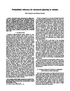
Figure 2: Schematic illustration of how the δ clocks for each measurement h and ¬h evolve. The two deltas are a summation of transmission time and a local clock period. The sprinkler binary variable is queried at noon (12:00) and at midnight (24:00). The corresponding code is in Figure 3. process, the age of information can be helpful if one wants to infer the distribution of random variables. Tracking the causal history of events might then be avoidable, yielding a more scalable system. Furthermore a Bayesian probabilistic framework allows to incorporate out-of-order processing in terms of uncertainty instead of requiring explicit conflict resolution.

3.4 Parallelized Optimization (Machine-Learning) Different techniques for parallelization and distribution of machine learning algorithms have been explored, but in general they are assumed to happen in a setting with bounded delays and most often have some form of strong centralized coordination. These approaches do not model time as a first-class (explicit) concept, but rather hide it in the implicit mechanics of the optimization algorithm, e.g. in [12]. While the literature is increasingly rich, it does not consider a fully distributed setting to our knowledge. It is instead focused on parallelization in large-scale computing clusters and is seen more as an engineering problem than as a limitation in modeling distributed inference.

4 Experiment We want to demonstrate with our toy example for the sprinkler with its humidity sensor how we can use the probabilistic programming system Anglican [1] to model our delay mechanism in Figure 3. In reality we would measure all sensor data including the delays and actual measurements of the humidity sensor in a supervised setting and then use the dataset for inference of λδ . From its distribution we can immediately infer whether the sensor information is even useful for the random variables we observe. If we view the interaction

5

( with−primitive−procedures [ exponential−decay ] ( d e f q u e r y s p r i n k l e r − w i t h − h u m i d i t y − d e l a y [ data ] ( l e t [ lambda−delta ( sample ( u n i f o r m − c o n t i n u o u s 0 1 . 0 ) ) ] ( l o o p [ [ d & r ] data ] ( i f ( not d ) lambda−delta ( l e t [ [ s−1 s−2 ] d h−1−t ( sample ( u n i f o r m − c o n t i n u o u s 0 3 ) ) ; ; 0 : 0 0 − 3 : 0 0 h−1−delay (− 12 h−1−t ) h−1 t r u e ; ; r a i n e d e a r l y h−1∗ ( e x p o n e n t i a l − d e c a y lambda−delta h−1−delay h−1 0 . 2 ) ( o b s e r v e ( f l i p (− 1 h−1 ∗ ) ) s−1 ) h−2−t ( sample ( u n i f o r m − c o n t i n u o u s 12 1 5 ) ) ; ; 1 2 : 0 0 − 1 5 : 0 0 h−2−delay (− 24 h−2−t ) h−2 f a l s e ; ; n o t l a t e h−2∗ ( e x p o n e n t i a l − d e c a y lambda−delta h−2−delay h−2 0 . 2 ) ( o b s e r v e ( f l i p (− 1 h−2 ∗ ) ) s−2 ) ] ( recur r ) ) ) ) ) ) )

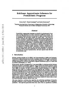
Figure 3: Generative model in Anglican ([1]). We have implemented our exponential decay mechanism in an external procedure. The query form depends on data about the desired sprinkler behaviour. The loop then conditions the posterior distribution over λδ and returns samples. Note that we turn on the sprinkler for s-1 and s-2 with inverse probability that it is humid. We have put a uniform distribution over λδ since we have no good guess what it should be except that values larger than 1 are unlikely. We turn the sprinkler on at 12h and at 24h, each time depending on whether it is humid. We also have no guess (yet) of how the sending time of the humidity sensor is distributed, so we take the uniform distribution for simplicity.

6

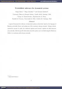
Figure 4: Using three datasets over sprinkler probabilities in blue, orange and green, we can infer distributions over λδ , showing how quickly our observations from the humidity sensor become irrelevant. between the random variables as stochastic processes in time, we want to infer how long they are correlated in some way. For demonstration purposes we have done a comparison on three synthetic datasets of 1000 binary sprinkler measurements as the following cases: We observe a 1. never sprinkling at noon, always sprinkling at night with perfect correlation to humidity 2. sprinkling at noon with probability 0.2 and at night with probability 0.9 and 3. sprinkling always with the same probability 0.8. As can be seen by comparison in Figure 4 there should be no decay in information in 1. (blue) and hence λδ is practically zero. For 2. (orange) the information is still valuable, but does not perfectly describe the sprinkling behaviour. The humidity changes by factors not captured in the sensor data. In 3. (green) the decay is so strong, that after roughly 10 hours it is close to the empirical average of sprinkling behaviour (fig. 5). We gain several practical insights from each distribution over λδ . First we do not need to hardcode timing decisions in our inference mechanism. Instead, by leveraging the standard techniques of probabilistic inference we can immediately make an informed guess of what the decay should be if we want to run the inference in an unsupervised setting. Second we can evaluate how useful the sensor really is and make adjustments to our probabilistic inference system. In case 3. we could try to run the sensor either closer to the sprinklers query time or more often to get a better time estimate. We can also speculate whether the humidity sensor is sending the right signal or might be worseless. That way we could add for example additional sensors to the system to improve its predictive power.

5 Outlook The incorporation of delays into a sound mathematical framework is only a first step towards full incorporation of time and process into graphical models. Stochastic processes like Markov chains have been traditionally used to describe such systems evolving in continuous time. Loops (memory) can occur in general, complicated graphical models.

7

Figure 5: For λδ = 0.25 and our prior probability of humidity p = 0.2, can see how our certain observation of humidity decays towards the prior value. At zero delay we make our observation with probability 1, while after 10 hours we are close to the probability under unconditioned behaviour of the sprinkler. This curve matches the infered behaviour of case 3.

8

Here, convergence properties of loopy belief-propagation might be transferable. Nonstationary behavior of the delays also needs consideration. Once a model for distributed and decoupled statistic inference has been developed, a universal layer of statistic inference is available. This will allow different parties to share information with minimum effort, similar to recent open replication systems 7 .

5.1 Replication Furthermore, models, i.e. subgraphs, can be replicated as running, distributed copies of the same subgraphs, and information can propagate between them. This will require regular exchange over the inferred parameters of the underlying statistical manifold, e.g. using some form of gossip. Maybe some lessons from Riemannian optimization can be applied here [13] [14].

5.2 Joint systems The composition with digital eventual consistent systems (e.g. datatypes to collect factual data) will be challenging, as a bridge between discrete and continuous information needs to be found to do joint computation without inducing conflicts on the digital side.

5.3 Differential privacy The resulting systems might also share sensible information between separate parties and newly evolving methods for differential privacy will be applicable to a distributed probabilisitic system [15].

5.4 Acknoweledgements Part of this work has been supported by the H2020 LightKone Project8 .

References [1]

D. Tolpin, J. W. van de Meent, H. Yang, and F. Wood, “Design and implementation of probabilistic programming language anglican,” ArXiv preprint arXiv:1608.05263, 2016.

[2]

D. Barber, Bayesian Reasoning and Machine Learning. Cambridge University Press, 2012.

[3]

C. M. Bishop and N. M. Nasrabadi, “Pattern Recognition and Machine Learning,” J. Electronic Imaging, vol. 16, no. 4, p. 049 901, 2007. doi: 10.1117/1.2819119. [Online]. Available: http://dx.doi.org/10.1117/1.2819119.

[4]

Y. Gal, “Uncertainty in deep learning,” PhD thesis, University of Cambridge, 2016.

7 8

e.g., https://ipfs.io or http://replikativ.io, the latter is a project of the author. https://www.lightkone.eu/

9

[5]

M. D. H. Stephan Mandt and D. M. Blei, “Stochastic gradient descent as approximate bayesian inference,” 2017. [Online]. Available: https://arxiv.org/abs/ 1704.04289.

[6]

T. Broderick, N. Boyd, A. Wibisono, A. C. Wilson, and M. I. Jordan, “Streaming variational bayes,” in Advances in Neural Information Processing Systems 26, C. J. C. Burges, L. Bottou, M. Welling, Z. Ghahramani, and K. Q. Weinberger, Eds., Curran Associates, Inc., 2013, pp. 1727–1735. [Online]. Available: http : //papers.nips.cc/paper/4980-streaming-variational-bayes.pdf.

[7]

D. Tran, R. Ranganath, and D. M. Blei, “Deep and hierarchical implicit models,” CoRR, vol. abs/1702.08896, 2017. [Online]. Available: http://arxiv.org/abs/ 1702.08896.

[8]

A. Radul, Propagation networks: A flexible and expressive substrate for computation, ser. CSAIL Technical Reports. 2009. [Online]. Available: http : / / hdl . handle.net/1721.1/49525.

[9]

M. Shapiro, N. M. Pregui¸ca, C. Baquero, and M. Zawirski, “Conflict-free replicated data types,” in Stabilization, Safety, and Security of Distributed Systems 13th International Symposium, SSS 2011, Grenoble, France, October 10-12, 2011. Proceedings, 2011, pp. 386–400. doi: 10.1007/978-3-642-24550-3_29. [Online]. Available: http://dx.doi.org/10.1007/978-3-642-24550-3_29.

[10]

H. A. P. B. A. Davey, Introduction to lattices and order, 2nd. Cambridge University Press, 2002, isbn: 0521784514,9780521784511.

[11]

L. Kuper and R. R. Newton, “Lvars: Lattice-based data structures for deterministic parallelism,” in Proceedings of the 2nd ACM SIGPLAN workshop on Functional high-performance computing, Boston, MA, USA, FHPC@ICFP 2013, September 25-27, 2013, 2013, pp. 71–84. doi: 10.1145/2502323.2502326. [Online]. Available: http://doi.acm.org/10.1145/2502323.2502326.

[12]

S. Teerapittayanon, B. McDanel, and H. T. Kung, “Distributed deep neural networks over the cloud, the edge and end devices,” in 37th IEEE International Conference on Distributed Computing Systems, ICDCS 2017, Atlanta, GA, USA, June 5-8, 2017, 2017, pp. 328–339. doi: 10.1109/ICDCS.2017.226. [Online]. Available: https://doi.org/10.1109/ICDCS.2017.226.

[13]

S. Bonnabel, “Stochastic gradient descent on riemannian manifolds,” IEEE Trans. Automat. Contr., vol. 58, no. 9, pp. 2217–2229, 2013. doi: 10.1109/TAC.2013. 2254619. [Online]. Available: http://dx.doi.org/10.1109/TAC.2013.2254619.

[14]

N. T. Trendafilov, “P.-A. absil, r. mahony, and r. sepulchre. optimization algorithms on matrix manifolds,” Foundations of Computational Mathematics, vol. 10, no. 2, pp. 241–244, 2010. doi: 10.1007/s10208-009-9051-7. [Online]. Available: http://dx.doi.org/10.1007/s10208-009-9051-7.

10

[15]

C. Dwork and A. Roth, “The algorithmic foundations of differential privacy,” Foundations and Trends in Theoretical Computer Science, vol. 9, no. 3-4, pp. 211– 407, 2014. doi: 10.1561/0400000042. [Online]. Available: http://dx.doi.org/ 10.1561/0400000042.

11