time series modeling and designing of artificial neural

TIME SERIES MODELING AND DESIGNING OF ARTIFICIAL NEURAL NETWORK (ANN) FOR REVENUE FORECASTING

NORFADZLIA BINTI MOHD YUSOF

UNIVERSITI TEKNOLOGI MALAYSIA

PSZ 19:16 (Pind. 1/97)

UNIVERSITI TEKNOLOGI MALAYSIA

BORANG PENGESAHAN STATUS TESIS♦ JUDUL : TIME SERIES MODELING AND DESIGNING OF ARTIFICIAL NEURAL NETWORK (ANN) FOR REVENUE FORECASTING

SESI PENGAJIAN: 2005/2006 Saya :

NORFADZLIA BINTI MOHD YUSOF (HURUF BESAR)

mengaku membenarkan tesis ( PSM / Sarjana / Doktor Falsafah )* ini disimpan di Perpustakaan Universiti Teknologi Malaysia dengan syarat-syarat kegunaan seperti berikut: 1. Tesis adalah hakmilik Universiti Teknologi Malaysia. 2. Perpustakaan Universiti Teknologi Malaysia dibenarkan membuat salinan untuk tujuan pengajian sahaja. 3. Perpustakaan dibenarkan membuat salinan tesis ini sebagai bahan pertukaran antara institusi pengajian tinggi. 4. **Sila tandakan ( √ )

√

SULIT

(Mengandungi maklumat yang berdarjah keselamatan atau kepentingan Malaysia seperti yang termaktub di dalam AKTA RAHSIA RASMI 1972)

TERHAD

(Mengandungi maklumat TERHAD yang telah ditentukan oleh organisasi/badan di mana penyelidikan dijalankan)

TIDAK TERHAD Disahkan oleh

___________________________ (TANDATANGAN PENULIS)

__________________________________________ (TANDATANGAN PENYELIA)

Alamat Tetap: 18, JALAN SUKUN SUNGAI ROKAM 31350, IPOH PERAK

PM DR. SITI MARIYAM BINTI SHAMSUDDIN (Nama Penyelia)

Tarikh:

Tarikh:

CATATAN:

30 JUN 2006

30 JUN 2006

* Potong yang tidak berkenaan. ** Jika tesis ini SULIT atau TERHAD, sila lampirkan surat daripada pihak berkuasa/organisasi berkenaan dengan menyatakan sekali sebab dan tempoh tesis ini perlu dikelaskan sebagai SULIT atau TERHAD. ♦ Tesis dimaksudkan sebagai tesis bagi Ijazah Doktor Falsafah dan Sarjana secara penyelidikan, atau disertasi bagi pengajian secara kerja kursus dan penyelidikan, atau Laporan Projek Sarjana Muda (PSM).

“We hereby declare that we have read this project report and in our opinion this project report is sufficient in terms of scope and quality for the award of the degree of Master of Science (Computer Science)”

Signature

:

…………………………………………………..

Name of Supervisor I

:

Assoc. Prof. Dr. Siti Mariyam Binti Shamsuddin

Date

:

…………………………………………………..

Signature

:

…………………………………………………..

Name of Supervisor II

:

Puan Roselina Binti Sallehuddin

Date

:

…………………………………………………..

TIME SERIES MODELING AND DESIGNING OF ARTIFICAL NEURAL NETWORK (ANN) FOR REVENUE FORECASTING

NORFADZLIA BINTI MOHD YUSOF

A project report submitted in partial fulfillment of the requirements for the award of the degree of Master of Science (Computer Science)

Faculty of Computer Science and Information System Universiti Teknologi Malaysia

JUNE 2005

ii

“I declare that this project report entitled “Time Series Modeling And Designing of

Artifical Neural Network (ANN) for Revenue Forecasting” is the result of my own research except as cited in the references. The project report has not been accepted for any degree and is not concurrently submitted in candidature of any other degree.”

Signature

:

………………………………

Name

:

Norfadzlia Binti Mohd Yusof

Date

:

………………………………

iii

To my beloved and supportive family

iv

ACKNOWLEDMENT

I would like to express the deepest appreciation to my major advisor, Assoc. Prof. Dr. Siti Mariyam Binti Shamsuddin for her direction, assistance, and guidance in the accomplishment of this project report. Words are inadequate to express my thanks to Dr. Siti Mariyam. I have yet to see the limits of her wisdom, patience, and selfless concern for her students. In particular, Dr. Siti Mariyam’s recommendations and suggestions have been invaluable for the study and for research improvement. Many thank to my co-supervisor, Puan Roselina Binti Sallehuddin for her enthusiasm in sharing her knowledge and expertise. Without their guidance and persistent help this dissertation would not have been possible.

Many thanks to Encik Zaily Bin Ayub and Tuan Haji Md. Shah whom have always been very generous with their time, and they puts a lot more effort than necessary into teaching me about the data analysis and supplied me with the revenue data. I would also like to express thanks to my examiners for their useful comments.

Special thanks to all my family members (abah, mama, abang, adik, eleen, tok and paksu) for giving me their constant encouragement, strength, support and love I needed to complete my goals. I am very thankful to my beloved twin’s sister Norfadzila Binti Mohd Yusof, who always encouraged me to do my best. I also would like to express my gratitude to the lecturers who made my experience in graduate school worthwhile.

Lastly, I would like to dedicate this project report to the memory of my beloved grandfather that passed away on 15th May 2006, as I was nearing completion of this project report. Memory nourishes the heart, and grief abates.

v

ABSTRAK

Rangkaian

neural

telah

mendapat

perhatian

dalam

teori

unjuran.

Walaubagaimanapun, pemilihan pelbagai parameter untuk membina model unjuran rangkaian neural bermakna proses merekanya masih melibatkan kaedah cuba jaya. Objektif kajian ini ialah untuk menyiasat kesan pengaplikasian pelbagai nilai nod input, fungsi-fungsi penggiatan dan teknik-teknik transformasi data ke atas pelaksanaan unjuran siri masa pungutan hasil oleh rangkaian neural rambatan balik. Dalam kajian ini, beberapa teknik transformasi data telah digunakan untuk mengeluarkan komponen tidak pegun di dalam siri masa data, dan kesannya ke atas proses pembelajaran dan menghasilkan unjuran menggunakan model rangkaian neural dianalisa. Kaedah cuba jaya digunakan di dalam kajian ini untuk mendapatkan jumlah nod input yang sesuai begitu juga dengan jumlah nod terselindungnya yang ditentukan melalui teorem Kolmogorov. Kajian ini juga menumpukan kepada perbandingan penggunaan fungsi logaritma dan model rangkaian neural cadangan yang menggabungkan fungsi sigmoid di nod lapisan terselindung dan fungsi logaritma di lapisan nod output, dengan fungsi sigmoid sebagai fungsi penggiatan pada nod-nod tersebut. Kaedah eksperimen validasi-silang digunakan dalam kajian ini untuk meningkatkan keupayaan pengitlakan rangkaian neural. Hasil kajian ini menunjukkan bahawa model rangkaian neural yang mempunyai jumlah nod input yang kecil sejajar dengan saiz struktur rangkaiannya yang kecil berjaya menjana unjuran yang baik walaupun ia sengsara daripada penumpuan yang lambat. Fungsi penggiatan sigmoid mengurangkan kekompleksan rangkaian neural serta menjanakan penumpuan terpantas dan keupayaan unjuran yang baik di dalam hampir keseluruhan eksperimen. Kajian ini juga menunjukkan prestasi unjuran daripada rangkaian neural dapat ditingkatkan dengan mengunakan teknik transformasi data yang sesuai.

vi

ABSTRACT

Artificial neural networks (ANN) have found increasing consideration in forecasting theory. However, the large numbers of parameters that must be selected to develop ANN forecasting model have meant that the design process still involves much trial and error. The objective of this study is to investigate the effect of applying different number of input nodes, activation functions and pre-processing techniques on the performance of backpropagation (BP) network in time series revenue forecasting. In this study, several pre-processing techniques are presented to remove the non-stationary in the time series and their effect on ANN model learning and forecast performance are analyzed. Trial and error approach is used to find the sufficient number of input nodes as well as their corresponding number of hidden nodes which obtain using Kolmogorov theorem. This study compares the used of logarithmic function and new proposed ANN model which combines sigmoid function in hidden layer and logarithmic function in output layer, with the standard sigmoid function as the activation function in the nodes. A cross-validation experiment is employed to improve the generalization ability of ANN model. From the empirical findings, it shows that an ANN model which consists of small number of input nodes and smaller corresponding network structure produces accurate forecast result although it suffers from slow convergence. Sigmoid activation function decreases the complexity of ANN and generates fastest convergence and good forecast ability in most cases in this study. This study also shows that the forecasting performance of ANN model can considerably improve by selecting an appropriate pre-processing technique.

vii

TABLE OF CONTENTS

CHAPTER

1

TITLE

PAGE

DECLARATION

ii

DEDICATION

iii

ACKNOWLEDGEMENT

iv

ABSTRAK

v

ABSTRACT

vi

TABLE OF CONTENT

vii

LIST OF TABLES

xi

LIST OF FIGURES

xiv

LIST OF SYMBOLS

xvii

LIST OF ABBREVIATIONS

xviii

LIST OF TERMINOLOGIES

xix

LIST OF APPENDICES

xxi

INTRODUCTION

1

1.1

Introduction

1

1.2

Problem Background

2

1.3

Problem Statement

5

1.4

Study Aims

5

1.5

Objectives

6

1.6

Scopes of Study

6

1.7

Significance of the Study

7

1.8

Organization of the Report

8

viii 2

3

LITERATURE REVIEW

9

2.1

Introduction

9

2.2

Overview of Royal Malaysian Customs Department

10

2.3

Revenue Collection

12

2.4

Introduction to Forecasting

14

2.5

ANN in Time Series Forecasting

17

2.6

Traditional Time Series Forecasting

18

2.7

ANN versus Traditional Time Series Forecasting

19

2.8

Artificial Neural Network (ANN)

22

2.9

Feed-forward Neural Network

23

2.10 Multilayer Perceptron (MLP)

25

2.11 Backpropagation (BP) Algorithm

26

2.12 Designing an ANN Forecasting Model

30

2.13 Data Pre-processing Techniques

31

2.13.1 Visual Inspection

33

2.13.2 Scaling

33

2.13.3 Detrending

34

2.14 Creating Training, Validation and Test Set

36

2.15 ANN Paradigms

38

2.15.1 Number of Input Nodes

39

2.15.2 Number of Hidden Layers

39

2.15.3 Number of Hidden Nodes

40

2.15.4 Number of Output Nodes

41

2.15.4 Activation Function

41

2.16 Summary

46

METHODOLOGY

47

3.1

Introduction

47

3.2

Step 1: Variable Selection

50

3.3

Step 2: Data Collection

50

3.4

Step 3: Data Pre-processing

51

3.5

Step 4: Creating Training, Validation and Test Set

53

3.6

Step 5: ANN Paradigms

55

ix 3.7

Step 6: Evaluation Criteria

56

3.8

Step 7: ANN Training

57

3.8.1

Number of Training Iteration (Epoch)

61

3.8.2

Learning Rate and Momentum Term

61

3.9

4

Step 8: Implementation

62

3.10 Step 8: Result Analysis

62

3.11 Hardware and Software Specification

63

3.12 Summary

64

EXPERIMENTAL RESULT AND ANALYSIS

65

4.1

Introduction

65

4.2

Cross-Validation Experiment Set Up

67

4.3

Forecasting Result with Validation Set

70

4.4

ANN Models Learning Performance

82

4.5

Forecasting Performance with Test Set

93

4.6

Selection of Appropriate Data PreProcessing Technique and Optimal ANN

5

Paradigm with Test Set

102

4.7

Discussion

105

4.8

Summary

114

CONCLUSION

116

5.1

Discussion

116

5.2

Summary of Work

117

5.3

Contribution

119

5.4

Conclusion

121

5.5

Suggestions of Future Work

121

REFERENCES

123

APPENDIX A

128

APPENDIX B

129

APPENDIX C

130

x APPENDIX D

131

APPENDIX E

132

APPENDIX F

133

APPENDIX G

134

xi

LIST OF TABLES

TABLE NO.

TITLE

PAGE

2.1

Indirect taxes

13

2.2

The summarized steps in BP algorithm

29

2.3

Eight steps in designing an ANN forecasting model

30

2.4

Types of inputs

31

2.5

Activation functions

43

2.6

Mathematical definition of the activation functions

45

3.1

Revenue time series (January 1990 to February 1991)

51

3.2

Structure of the data matrix corresponding to the ANN model using 1 and 2 look-back periods

52

3.3

Data partitioning with two look-back periods

53

3.4

Input data partitioned

54

3.5

Target data partitioned

55

3.6

List of hardware

64

4.1

Features of three types of ANN model

66

4.2

Architectures of ANN model

66

4.3

Cross-validation experiments set up

68

4.4(a)

Forecasting accuracy of ANN models with validation set in raw values dataset

4.4(b)

Forecasting accuracy of ANN models with validation set in logs dataset

4.4(c)

72

Forecasting accuracy of ANN models with validation set in logs + first differences dataset

4.4(d)

71

74

Forecasting accuracy of ANN models with validation sets in logs + seasonal differences dataset

76

xii TABLE NO. 4.4(e)

TITLE Forecasting accuracy of ANN models with validation set in logs + first + seasonal differences dataset

4.4(f)

77

Forecasting accuracy of ANN models with validation set in logs + one step return dataset

4.4(g)

PAGE

79

Forecasting accuracy of ANN models with validation set in logs + one step return + seasonal differences dataset

4.5(a)

Forecasting accuracy of ANN models with training set in raw values dataset

4.5(b)

89

Forecasting accuracy of ANN models with training set in logs + one step return dataset

4.5(g)

87

Forecasting accuracy of ANN models with training set in logs + first + seasonal differences dataset

4.5(f)

86

Forecasting accuracy of ANN models with training set in logs + seasonal differences dataset

4.5(e)

84

Forecasting accuracy of ANN models with training set in logs + first differences dataset

4.5(d)

83

Forecasting accuracy of ANN models with training set in logs dataset

4.5(c)

81

90

Forecasting accuracy of ANN models with training set in logs + one step return + seasonal differences dataset 92

4.6(a)

Forecasting accuracy of optimal ANN models with validation set and test set in raw values dataset

4.6(b)

Forecasting accuracy of optimal ANN models with validation set and test set in logs dataset

4.6(c)

93

95

Forecasting accuracy of optimal ANN models with validation set and test set in logs + first differences dataset

4.6(d)

96

Forecasting accuracy of optimal ANN models with validation and test set in logs + seasonal differences dataset

4.6(e)

Forecasting accuracy of optimal ANN models with

97

xiii TABLE NO.

TITLE

PAGE

validation and test set in logs + first + seasonal differences dataset 4.6(f)

99

Forecasting accuracy of optimal ANN models with validation set and test set in logs + one step return dataset

4.6(g)

100

Forecasting accuracy of optimal ANN models with validation set and test set in logs + one step return + seasonal differences dataset

101

4.7

Best ANN model for revenue series

103

4.8

Simulation results for ANN models

104

4.9

Comparing the out-of-sample forecast evaluation results for different data pre-processing techniques.

4.10

Types of ANN model which produce best learning performances in cross-validation experiments

4.11

4.12

105

106

Types of ANN model which produce best forecast results in cross-validation experiments

110

Best ANN models

111

xiv

LIST OF FIGURES

FIGURE NO.

TITLE

PAGE

2.1

A taxonomy of ANNs architecture

10

2.2

Working of neuron

23

2.3

A feed-forward network

24

2.4

MLP network for one-step-ahead forecasting based on two lagged terms

2.5

26

Monthly revenue collection from January 1990 to December 2004

33

2.6

Three-way data splits

38

3.1

A general framework in proposed study

49

4.1

Cross-validation experiment work flow

69

4.2

Example of cross-validation experiment

70

4.3(a)

Forecasting accuracy of ANN models with validation set in raw values dataset

4.3(b)

Forecasting accuracy of ANN models with validation set in logs dataset

4.3(c)

73

Forecasting accuracy of ANN models with validation set in logs + first differences dataset

4.3(d)

72

75

Forecasting accuracy of ANN models with validation sets in logs + seasonal differences dataset 76

4.3(e)

Forecasting accuracy of ANN models with validation set in logs + first + seasonal differences dataset

4.3(f)

Forecasting accuracy of ANN models with

78

xv FIGURE NO.

TITLE validation set in logs + one step return

4.3(g)

PAGE 80

Forecasting accuracy of ANN models with validation set in logs + one step return + seasonal differences

4.4(a)

Learning performances of ANN models with training set in raw values dataset

4.4(b)

87

Learning performances of ANN models with training set in logs + seasonal differences dataset

4.4(e)

85

Learning performances of ANN models with training set in logs + first differences dataset

4.4(d)

84

Learning performances of ANN models with training set in logs dataset

4.4(c)

82

88

Learning performances of ANN models with training set in logs + first + seasonal differences dataset

4.4(f)

Learning performances of ANN models with training set in logs + one step return dataset

4.4(g)

89

91

Learning performances of ANN models with training set in logs + one step return + seasonal differences dataset

4.5(a)

Forecasting accuracy of optimal ANN models with test set in raw values dataset

4.5(b)

98

Forecasting accuracy of optimal ANN model with test set in logs + first + seasonal differences dataset

4.5(f)

97

Forecasting accuracy of optimal ANN models with test set in logs + seasonal differences dataset

4.5(e)

95

Forecasting accuracy of optimal ANN models with test sets in logs + first differences dataset

4.5(d)

94

Forecasting accuracy of optimal ANN models with test set in logs dataset

4.5(c)

92

99

Forecasting accuracy of optimal ANN models with test set in logs + one step return dataset

100

xvi FIGURE NO. 4.5(g)

TITLE

PAGE

Forecasting accuracy of optimal ANN models with test set in logs + one step return + seasonal differences dataset

102

4.6(a)

Sigmoid model learning performance

107

4.6(b)

Logarithmic model learning performance

108

4.6(c)

Siglog model learning performance

108

4.7(a)

ANN out-of-sample one-step forecasts using raw data

4.7(b)

ANN out-of-sample one-step forecasts using data after pre-processing with log transformation

4.8

112

113

Plotting of target data in raw values and logs dataset

113

xvii

LIST OF SYMBOLS

Wij

-

Weight connected between node i and j

W jk

-

Weight connected between node j and k

θj

-

Bias of node j

θk

-

Bias of node k

netj

-

Summation of sum of input for node j multiplied by the corresponding weights between node i and node j and bias j

netk

-

Summation of sum of input of node k multiplied by the corresponding weights between node j and node k and bias k

oi

-

Output of node i

oj

-

Output of node j

ok

-

Output of node k

tj

-

Target output value at node j

tk

-

Target output value at node k

Wij (t )

-

Weight from node i to node j at time t

W jk (t )

-

Weight from node j to node k at time t

∆ Wij

-

Weight adjustment between node i and j

∆ W jk

-

Weight adjustment between node j and k

η

-

Learning rate

α

-

Momentum term

δj

-

Error signal at node j

δk

-

Error signal at node k

xviii

LIST OF ABBREVIATIONS

ANN

-

Artificial Neural Network

BP

-

Backpropagation

MAPE

-

Mean Absolute Percentage Error

MLP

-

Multilayer Perceptron

MSE

-

Mean Squared Error

NN

-

Neural Network

RMSE

-

Root Mean Squared Error

xix

LIST OF TERMINOLOGIES

Backpropagation

-

A supervised learning method in which an output error signal is fed back through the network, altering connection weights so as to minimize error.

Connection

-

A link between nodes used to pass data from one node to the other. Each connection has an adjustable value called a weight.

Generalization

-

A neural network’s ability to respond correctly to data not used to train it.

Global minima

-

The unique point of least error during gradient descent, metaphorically the true “bottom” of the error surface.

Gradient descent

-

A learning process that changes a neural networks weights to follow the steepest path toward the point of minimum error.

Input layer

-

A layer of nodes that forms a passive conduit of data entering a neural network.

Hidden layer

-

A layer of nodes not directly connected to a neural networks input or output.

Local minima

-

A point of regionally low error during gradient descent, a metaphorical dent in the error surface.

Over-fitting

-

A neural network’s tendency to learn random details in the training data in addition to the underlying function. A network that simply memorizes may fail to generalize.

Node

-

A single neuron-like element in a neural network.

Output layer

-

The layer of nodes that produce the neural network result.

Supervised

-

A learning process requiring a labeled training set.

learning

xx Target output

-

A “correct” result included with each input pattern in a training or testing data set.

Testing

-

A process for measuring a neural network’s performance, during which the network’s passes through an independent data set to calculate a performance index. It does not change its weights.

Training

-

A process during which a neural network passes through a data set repeatedly, changing the values of its weights to improve its performance.

Weight

-

An adjustable value associated with a connection between nodes in a neural network.

xxi

LIST OF APPENDICES

APPENDIX

TITLE

PAGE

A

Revenue Raw Values Dataset

128

B

Revenue Logs Dataset

129

C

Revenue Logs + First Differences Dataset

130

D

Revenue Logs + One Step Return

131

E

Revenue Logs + Seasonal Differences

132

F

Revenue Logs + First + Seasonal Differences Dataset

133

G

Revenue Logs + One Step Return + Seasonal Differences Dataset

134

CHAPTER 1

INTRODUCTION

1.1

Introduction

Knowing future better has attracted many people for thousands of years. The forecasting methods vary greatly and will depend on the data availability, the quality of models available, and the kinds of assumptions made, amongst other things. Generally speaking, forecasting is not an easy task and therefore it has attracted many researchers to explore it.

Artificial neural network (ANN) has found increasing consideration in forecasting theory, leading to successful applications in various forecasting domains including economic (Yao, 2002), business (Crone et al., 2004), financial (Lam, 2004), and many more. ANN can learn from examples (pass data), recognize a hidden pattern in historical observations and use them to forecast future values. In addition to that, they are able to deal with incomplete information or noisy data and can be very effective especially in situations where it is not possible to define the rules or steps that lead to the solution of a problem.

2 Despite of many satisfactory characteristics (Zhang et al, 1998), of ANNs, building an ANN model for a particular forecasting problem is a nontrivial task. Several authors such as Bacha and Meyer (1992), Tan and Witting (1993), Kaastra and Boyd (1996), Zhang et al. (1998), Plummer (2000), Xu and Chen (2001), Lam (2004) have provided an insight on issues in developing ANN model for forecasting. These modeling issues must be considered carefully because it may affect the performance of ANNs. Based on their studies, some of the discussed modeling issues in constructing ANN forecasting model are the selection of network architecture, learning parameters and data pre-processing techniques applies to the time series data.

Thus, this study uses a BP network to forecast future revenue collection for Royal Malaysian Customs Department. This study examines the effect of network parameters through trial and error approach by varying network structures based on the number of input nodes, activation functions and data pre-processing in designing of BP network forecasting model.

1.2

Problem Background

ANNs promise attractive feature to various forecasting domains: being a data driven learning machine as opposed to conventional model-based approaches, permitting universal approximation of arbitrary linear or non-linear functions, and therefore offering great flexibility in learning the generator of noisy data from examples and generalizing structure from it without priori assumptions (Zhang et al., 1998). However, the nontrivial task of modeling ANNs for a particular prediction problem is still considered to be as much an art as a science (Zhang et al., 1998), as the combination of choices may significantly impact on the networks ability to extrapolate results.

3 Due to their flexibility, neural networks lack a systematic procedure for model building. Therefore obtaining a reliable neural model involves selecting a large number of parameters experimentally through trial and error (Kaastra and Boyd, 1996). The performance of ANNs in forecasting is influenced by ANN modeling, that is the selection of the most relevant network architecture and network design. Poor selection of parameter settings can lead to slow convergence and incorrect output (Kong and Martin, 1995).

One critical decision is to determine the

appropriate network architecture, that is, the number of layers, the number of nodes in this layer, and the number of arcs which interconnect with the nodes. The network design decision include the selection of activation function in the hidden and output neurons, the training algorithm, data transformation or normalization method, training and test set, and performance measures.

When applying an ANN model in a real application, attention should be taken in every single step. The usage and training of ANN is an art. One successful experiment says nothing for real application. Zhang (1992), Tan and Witting (1993), Kong and Martin (1995), had focused their studies on parametric effects on building a BP network for a particular forecasting problem. Kaastra and Boyd, (1996), have provided a practical introductory guide in the design of ANN for forecasting financial and economic time series data. The issues on modeling fully-connected feed-forward networks for forecasting had been discussed by Zhang et al. (1998). Maier and Dandy (2000), have review the modeling issues and outlined the steps that should be followed in developing ANN model for predicting and forecasting water resource variables.

When BP algorithm was introduced in 1986, there has been much development in the use of ANNs for forecasting by a number of researchers for examples Zhang (1992), Tan and Witting (1993), Yu and Chen (1993), Kong and Martin (1995), Yu (1999), Lopes et al. (2000), More and Deo (2003), Crone et al. (2004).

4 BP network is characterized by its robustness, its ability to generalize, learn and to be trained (Kong and Martin, 1995). Although this algorithm is widely used and recognized as a powerful tool for training feed-forward neural network, it suffers from slow convergence process, or long training time (Nguyen et al., 1999, Bilski, 2000, Xu and Chen, 2001, Kamruzzaman and Aziz, 2002, Kodogiannis and Anagnostakis, 2002). One of the identified reason of slow convergence is the used of sigmoid activation function in hidden and output layer of BP network (Bilski, 2000, Kamruzzaman and Aziz, 2002). A number of researches have been done in order to improve the convergence rate of BP learning. Therefore, several approaches have been developed in order to speed up the convergence.

Fnaiech et al. (2002) have summarized the approaches for increasing the BP convergence speed onto seven cases: the weight updating procedure, the choice of optimization criterion, the use of adaptive parameters, estimation of optimal initial conditions, reducing the size of problem, estimation of optimal ANN structure and application of more advanced algorithms. According to Kamruzzaman and Aziz (2002), approaches to accelerate BP learning include, selection of better cost function, dynamics variation of learning rate and momentum and selection of better activation function of the neurons. Bilski (2000); Kamruzzaman and Aziz (2002), have proposed new activation functions in order to accelerate BP learning process.

Several other approaches also have been implemented in forecasting problem. For example, Xu and Chen (2001), have employed the fast convergence algorithm the quasi-Newton method to expedite the training process in short-term load forecasting problem. Another work by Kodogiannis and Anagnostakis (2002), have adopted the adaptive learning rate BP network, which relates the learning rate with the total error function in order to accelerate the convergence speed of standard BP in short-term load forecasting.

This research attempts to design an ANN model for revenue time series forecasting. A BP network forecasting model is constructed to test its forecasting

5 capability by implementing modification on several network parameters. The modeling issues discussed in this study are focused on network paradigms (specifically to determine sufficient number of input node and activation function) and data pre-processing. The learning ability and forecast result produce by ANN models are evaluated and examined.

1.3

Problem Statement

The problem statement of this study is as follow:

How the selection of these parameters in network modeling namely: number of input nodes, activation functions and data pre-processing techniques may affect the forecasting capability of ANN in time series revenue forecasting?

1.4

Study Aims

This study aims to provide a step by step methodology for designing ANN for revenue time series forecasting. This research also attempts to explore: a) the effectiveness of data pre-processing technique on ANN modeling and forecasting performance. b) the generalization capability of the ANN by varying the network structure.

6 1.5

Objectives

1. To design and develop ANN model which combines sigmoid activation function in hidden layer and logarithmic activation function in output layer.

2. This research attempts to understand the network parameters by varying them and observing their effect on the network. Specifically, the parametric effect of varying the: •

data pre-processing technique

•

number of nodes in the input layer of ANN model

•

activation function in hidden and output layers of ANN model

are monitored in an attempt to develop an understanding of their effect on building a revenue forecasting model.

1.6

Scopes of Study

The scopes of this study are as follow:

1. Real time series data of monthly revenue collection obtained from Royal Malaysian Customs Department in Putrajaya from January 1990 to December 2004 are used as input to the ANN model.

2. The MLP network with three layers (one hidden layer, an input and an output layer) are used.

3. Trial and error design procedures are employed to arrive at an acceptable structure and parameter namely: data pre-processing technique, number of input node and activation function of ANN model.

7 4. Different data pre-processing techniques are presented to deal with irregularity components exist in time series data and their properties are evaluated by performing one step-ahead revenue forecasting using neural network.

5. The network input nodes are varied from 1 to 11 nodes to see its effect onto the network while the number of hidden node is obtained by using Kolmogorov theorem.

6. The output of the network is the forecast of one-step-ahead revenue collection.

7. Activation functions used for observation and combination are the sigmoid function and the logarithmic function.

8. Economic and other outside factors are not considered and included in the estimation.

9. Standard BP program is developed in Windows environment using Microsoft Visual C++ 6.0.

1.7

Significance of the Study

The study examines the effectiveness of BP network model as an alternative tool for forecasting. This study provides a practical introductory guide in the design of an ANN for forecasting time series data. We use the time series corresponding to the revenue collection in Royal Malaysian Customs Department to illustrate this process. This research attempts to study the behavior of ANN models when several of its parameters are altered. The relevancy of applying difference non-linear activation functions in hidden and output layers of ANN model is also examined in this study.

8 1.8

Organization of the Report

This report consists of five chapters. Chapter 1 presents the introduction of the study. Chapter 2 presents an appropriate literature and review on forecasting, ANN in time series forecasting, traditional time series forecasting, performance comparison between ANN and traditional time series forecasting technique from the past researched, explanation of ANN concept including network structure, BP algorithm and the affect of activation functions to BP learning. Chapter 3 discusses on the methodology used in this study. Chapter 4 provides experimental results and analysis of the obtained results. Chapter 5 draws the conclusion and suggestions for future work.

CHAPTER 2

LITERATURE REVIEW

This chapter reviews works that are related to time series forecasting using traditional methods and ANN techniques. Basically, reviews will be on overview of Royal Malaysian Customs Department, revenue collection, forecasting, application of ANNs in time series forecasting, traditional time series forecasting, ANN versus traditional time series forecasting, an overview of ANN and its architecture, learning algorithm, ANN forecasting model design methodology and lastly the several issues that are studied in this research.

2.1

Introduction

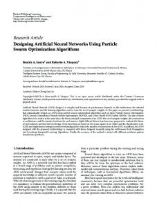
Neural networks (NN), or more precisely ANNs are a branch of artificial intelligence. Multilayer perceptrons (MLP) form one type of ANN as illustrated in the taxonomy in Figure 2.1. The MLP has been applied to wide variety of tasks, all of which can be categorized as prediction, function approximation, or pattern classification. Prediction involves forecasting of future trends in a time series of data given current and previous conditions. The BP is the most computationally straightforward algorithm for training the MLP.

10

Figure 2.1

Taxonomy of ANN architecture

Recently, ANNs have been investigated as a tool for time series forecasting. A survey of the literature is given in Zhang et al. (1998). The most popular class, used exclusively in this study, is the MLP, a feed-forward network trained by BP. Thus this study will employ this type of ANNs in the proposed forecasting problem.

2.2

Overview of Royal Malaysian Customs Department

The vision of Royal Malaysian Customs Department is to be a respected, recognized and a world class customs administration. The missions of Royal Malaysian Customs Department are: 1) To collect taxes and to provide customs facilitation to the trade and industrial sectors. 2) To improve compliance with the national legislations in order to protect national economic, social and security interest.

The primary focuses of Royal Malaysian Customs Department are: 1) To perform the function of revenue collection of indirect taxes competently, impartially and fairly yet efficiently.

11 2) To increase customs facilitation in congruence with country’s industrial and trade activities towards the national corporate concept. 3) To ensure a more effective customs monitoring system that safeguards the country’s economic, social and security interests. 4) To acquire effectively management resources skills for the significant functions of the department.

This department consists of 7 divisions. Each division is divided into several branches and units that give services and run particular jobs in order to fulfill the vision and mission of Royal Malaysian Customs. The divisions are: 1) Corporate Planning. 2) Information Technology. 3) Finance and Human Resource Management. 4) Internal Tax. 5) Customs. 6) Technical Services. 7) Preventive.

The Technical Services division is responsible for the classification of goods in the determination of tariff rates applicable. It is also responsible for the valuation of goods imported/exported and the determination of the weekly exchange rates for customs purposes. Apart from this, the review and drafting of legislations relating to customs matters are also handled by this division.

All goods imported/exported and locally manufactured/produced goods are classified under the Customs Duties Order 1996 in accordance with the World Customs Organization (WCO) Harmonized System Nomenclature. The classification of goods is imperative in determining the correct rates of duty are levied and also to ensure the effective control of goods prohibited from importation or exportation.

12 The objectives of this division is to assist the department to achieve a target of revenue collection conform to legislation of Customs Act 1967, Sale Tax Act 1972, Service Tax Act 1975, Excise Act 1976, Free Zone Act and Unordinary Profit Levied Act 1998 by following the preserved Customer Charter. The Technical Services division is divided into 5 branches that are: 1) Licensed Premise Inspection. 2) Pasca Import. 3) Classification. 4) ABT/Acceleration. 5) Revenue Accounting.

The objectives of Revenue Accounting branch are: 1) To ensure no lost of revenue happened in the department, besides give serious attention on the carrying out of the collection system and the department revenue accounting where it must be done correctly, accurate and affective. 2) To verify the investigation of application – return back claim application/pull back duty/tax and petroleum production subsidy payment are done correctly, competent and accurate.

2.3

Revenue Collection

Royal Malaysian Customs Department is responsible to collect the country revenue. Hence, this department is required to do forecasting in order to project the total revenue collection that will be collected each month and year. This department collects the indirect taxes that are described in Table 2.1 below:

13 Table 2.1 : Indirect taxes Taxes Import duties

Description Record duties collection imposed on various kinds of imported articles/goods including addition tax and duties that collected from passengers whom bring in articles/goods to Malaysia.

Export duties

Record collection of duties imposed on various kinds of exported articles/goods.

Excise duties

Record collection of duties imposed on various kinds of manufactured articles/goods.

Domestic sales

Record collection of taxes imposed on selling domestic

taxes

articles/goods.

Import sales

Record collection of taxes imposed on selling import

taxes

articles/goods.

Article Vehicle

Record collection of levies imposed on vehicle that carries

levied

articles/goods.

Service taxes

Record collection of taxes imposed on selling service.

Miscellaneous

Record collection of miscellaneous taxes others objects listed

taxes

above. Its include gambling tax.

Federals taxes

Record collection of direct tax revenue and indirect tax revenue collected by or on behalf of federals.

Revenue

Total summation of monthly collection value of above listed

collection

objects. This variable is dependent variable.

By the projection, the department may prepare for an appropriate action plan not only in the department level but also in each state. The usage of preparing the revenue projection is important to the department to give a clear direction and guidance in efforts to collect the country revenue. The revenue collection is the total summation of all types of indirect taxes as mentioned above. The indirect taxes are collected daily and the total monthly collection is used to forecast the revenue collection in the future. Forecast is performed by the officer in the Revenue Accounting branch in each state and is presented twice a year (the first half year and

14 the second half year) in a conference between the state directors of Royal Malaysian Customs Department.

The headquarters of the Royal Malaysian Customs Department is situated in Putrajaya. The Accounting Branch in Putrajaya is responsible in calculating the revenue collection for whole state in Malaysia and used the data to forecast the revenue collection for the country in the future. The package that is used by this department in generating revenue projection is the Forecast Pro package. The forecasting method used by this department is automatic selected using the expert selection menu in the package. The method used is based on the forecasting result that generates the less error. Since the package is applying the statistical method in doing forecasting, thus this study tries to adopt the ANN model and evaluate its capability in forecasting the revenue collection by Royal Malaysian Customs Department.

2.4

Introduction to Forecasting

Forecasting or predicting future events is an attempt to forecast events by examining the past. Forecasting techniques may be based on experiences, judgmental, experts’ opinion or mathematical models that describe the pattern of past data. Since the world in which organizations operate has always been changing, forecasts have always been necessary.

Almost every organization, large and small, private and public, uses forecasting either explicitly or implicitly, because almost every organization must plan to meet the conditions of the future for which it has imperfect knowledge. The need for forecast cuts across all functional lines as well as across all types of organizations. Forecasts are needed in finance, marketing, personnel, and production

15 areas, in government and profit-seeking organizations, in small social clubs, and in national political parties.

Forecast may be classified in two ways: long term or short term and point forecast (prediction of an actual value) or interval forecast (prediction for a range of values). Long-term forecasts are necessary to set the general course of an organization for the long runs; they thus become the particular focus of top management. Short-term forecasts are used to design immediate strategies and are used by mid-management and first-line management to meet the needs of the immediate future. Ranaweera et al. (1995), has applied a BP network model and radial basis NN model for short-term load forecasting.

Forecasting methods can be classified according to whether they are qualitative or quantitative. Qualitative method (also known as judgmental methods) are used when historical data concerning the events to be forecasted are either scarce or unavailable, or when the events to be forecasted are affected by non-quantifiable information or by technological change. Basically these procedures involve using the experiences, judgments and opinion of experts in the field.

In contrast to qualitative methods, quantitative methods employ statistical analysis of past data at various points in time. The researchers identifies a pattern from the historical data, fits a mathematical model to that pattern, and then uses the estimated equation of that model to forecast points in the future. This approach relies on the assumption that the identified pattern will continue into the future. Quantitative methods can be grouped into two types that are time series model (univariate) and causal model (multivariate).

Time series models are based on the analysis of a chronological sequence of observations on a particular variable. The observations may be collected yearly,

16 quarterly, monthly, daily, hourly and so on. Many researches and studies have used the time series model with ANN forecasting and this will be discussed in section 2.5.

However, studies on ANN forecasting done by Kong and Martin (1995), Danh et al. (1999), Limsombunchai et al. (2004), have used more than one variable in their prediction and these variables are historical and time series data. This type of forecasting is also known as causal model. Causal model was developed based on the assumption that the variable to be forecasted can be explained by the behavior of another variable or a set of variables (independent variables). The purpose of the causal model is to discover the functional form of the relationship between all the variables and to use it to forecast future values of the variables of interest (dependent variables).

An important consideration of forecasting approach is the number of items to forecast. If we need to forecast a few series and wish to be able to improve the accuracy of the forecasts, then we should employ the iterative forecasting. Interactive forecasting is limited to a single variable at a time. This process will give the deepest insights into the data, and can sometimes improve forecasting accuracy. This process is time consuming and practical when a number of items to be forecast is limited, and we wish to give each variable individual attention. On the other hand, it is more efficient and time consuming to used the batch forecasting if we want to forecast hundreds or thousands of series.

The important step in dealing with time series data is to identify the basic patterns or components inherent in the data. Once these components have been identified, the methods that best describe these patterns can be employed. Time series usually consists of four basic components that are trend, cycle, seasonal variations and irregular fluctuations.

17 Trend is a persistent upward or downward movement of the data over a long period. It reflects the long-term growth or decline in the time series. If a time-series does not contain any trend component, the data is said to be stationary. Seasonal variation term refers to a pattern of change in the data that completes itself within a calendar year and then is repeated on a yearly basis. These variations exist when a time series is influenced by some seasonal factor such as customs or weather. Cycle is the upward and downward change in the data pattern that occurs over duration of two to twelve years or longer. A cycle is measured from peak to peak or trough to trough. Cycle is one of the most difficult components to forecast because of its longer time frame. Irregularity fluctuations are the erratic movements in a time series that have no set or definable pattern. They are also referred to as white noises. These fluctuations are usually caused by influenced of “outside” events on the data. These events are usually “one-time” occurrences that are themselves unpredictable.

This study will employ time series model using interactive forecasting approach to forecast the following month revenue collection will be collected by Royal Malaysian Customs Department.

2.5

ANN in Time Series Forecasting

In time series modeling, historical data are analyzed in an attempt to identify a data pattern, and then assuming that the pattern will continue in the future, it is extrapolated in order to produce forecasts.

Nguyen and Chan (2004) have considered only the historical production time series as the basis for predicting future production of oil in their study. Bodis (2004), in his thesis has applied the time series model to predict the index values of several major US and European stock markets and to forecast the stock prices of famous

18 gigantic US companies (especially from the IT field). The data use only the close prices in order to build up different indicators and to use as inputs of the NN.

Research project done by Shlens (1999), investigates the ability of ANNs to predict time series. The project examined two applications that are predicting electrical power demand and earthquake tremors in Los Angeles. The ANNs modeling power demand not only predicted the next day’s peak power demand, but also generated a 24-hour profile of the demand for the next day. These ANNs successfully outperformed the predictive ability of a system used by the Los Angeles Department of Water and Power (LADWP). But the ANN failed to predict the earthquake tremors due to the voluminous amount of data and better results may only be obtained through researching on-line feature extraction and data preprocessing.

The study done by Sahai et al. (2000), shown that ANN can be used to predict the seasonal and monthly mean rainfall over the whole of India, using only rainfall time series as inputs. Various statistics are calculated to examine the performance of the models and it is found that the models could be used as a forecasting tool on seasonal and monthly time scales. Several more examples of studies that implement time series model with ANN are Zhang (1992), Yu and Chen (1993), Tan and Witting (1993), Plummer (2000), Virili and Freisleben (2000), More and Deo (2003), Crone et al. (2004).

2.6

Traditional Time Series Forecasting

Time series forecasting analyzes past data and projects estimates of future data values. Basically, this method attempts to model a non-linear function by a recurrence relation derived from past values. The recurrence relation can then be used to predict new values in the time series, which hopefully will be good

19 approximations of the actual values. A detailed analysis and description of these models is beyond the scope of this paper. However, a short overview is presented as the results from these models are often compared with ANN performance.

There are two basic types of time series forecasting: univariate and multivariate. Univariate models, like Box-Jenkins, contain only one variable in the recurrence equation. Box-Jenkins is a complicated process of fitting data to appropriate model parameters. The equations used in the model contain past values of moving averages and prices. Box-Jenkins is good for short-term forecasting but requires a lot of data, and it is a complicated process to determine the appropriate model equations and parameters.

Multivariate models are univariate models expanded to "discover casual factors that affect the behavior of the data". As the name suggests, these models contain more than one variable in their equations. Regression analysis is a multivariate model which has been frequently compared with ANNs. Overall, time series forecasting provides reasonable accuracy over short periods of time, but the accuracy of time series forecasting diminishes sharply as the length of prediction increases.

2.7

ANN versus Traditional Time Series Forecasting

Interest in using ANNs for forecasting has led to a tremendous surge in research activities in the past decade. ANNs have shown to be an effective method for forecasting time series events. Traditional research in this area uses a network with a sequential iterative learning process based on the feed-forward BP approach. ANN is said to be simple to implement, solves most problems correctly, and is unfussy about how it is used (Kong and Martin, 1995).

20 Athiya (2001), in his paper has reviewed the problem of bankruptcy prediction using ANNs. According to the author it seen that ANNs are generally more superior to other techniques in many studies. Based on the result from the experiment done by Yu and Chen (1993), they have concluded that the ANN approach is an attractive alternative to traditional regression techniques as a tool for traffic prediction.

Xu et al. (2004), have used ANN in forecasting electricity market prices: The experimental results show that the ANN outperform from 11.4% to 64.6% superior to the traditional linear regression method. It seems that the proposed multilayer ANN can be very useful in predicting the electricity market prices of European Energy Exchange.

Another study on wind forecasting by More and Deo (2003), forecast the wind speed over the next time step of 1 month, 1 week and 1 day at two coastal locations in India have shown that ANN produces much more accurate forecasts than the traditional stochastic time series model of ARIMA. Although this study also implement recurrent ANN and it shows that the training algorithm of cascade correlation yield slightly more accurate forecasts as compared to BP but still BP performs better forecast than ARIMA.

Ranaweera et al. (1995), apply the radial basis function and BP network model for short-term load forecasting. The paper also outlined the theoretical limitations of conventional statistical methods. These limitations are: 1) The non-linear relationships of the input and output variables are difficult to capture. 2) The co-linearity problem of the input variables limits the number of these inputs that can be used in the model. 3) The models are not very flexible in the face of rapid system load changes.

21 ANNs can be seen as a wide class of flexible non-linear regression and discriminates models, data reduction models and non-linear dynamical system. For the purpose of economic forecasting ANNs have some clear advantages over regression analysis (Tal and Nazareth, 1995): 1) Flexibility: As opposed to a simple regression where linearity in parameter is imposed on the data, ANN are non-linear nature. As for non-linear econometrics procedures, while significant work has been done on non-linear minimization problems in applied mathematics, these, in most cases, require specific assumptions regarding the non-linear structure of the investigated relationship. ANN-based system does not require such prior knowledge. These characteristics enable the ANN approach capture relationships with a higher degree of complexity. 2) Simplicity: Given the non-parametric character of ANNs, no subject-domain knowledge is incorporated in the modeling process. This means, for example, that no prior knowledge and assumptions regarding the probability distribution of the data are needed when using ANNs. Such assumptions are necessary in regression analysis.

Based on the methodology analysis done by Zekic (2005), on ANN applications in stock market prediction it can concluded from previous research that: 1) ANNs are efficiency methods in the area of stock market predictions, but there is no "recipe" that matches certain methodologies with certain problems. 2) ANNs are most implemented in forecasting stock prices and returns, although stock modeling is very promising problem domain of its application. 3) Most frequent methodology is the BP algorithm, but the importance of integration of ANN with other artificial intelligence methods is emphasized by many authors. 4) Benefits of ANN are in their ability to predict accurately even in situations with uncertain data, and the possible combinations with other methods. 5) Limitations have to do with insufficient reliability tests, data design, and the inability to identify the optimal topology for a certain problem domain.

22 Reviews on the research of time series forecasting had reported the benefit of using ANN for time series forecasting in the different areas and applications. All of these researches implement MLP structure ANN and is trained using BP algorithm. Thus, this study will also employ the MLP structure NN and BP algorithm in the experiments.

2.8

Artificial Neural Network (ANN)

ANN technology is an advanced computerized system of information processing. In many discussions they are credited with operating in the same way as the human brain. This is clearly an overstatement. Although loosely inspired by the structure of the brain, current ANN technology is far from being able to simulate even a simple brain function. Nevertheless, ANNs do offer a computational approach that is potentially very effective in solving problems which do not lend themselves to analysis by conventional means. The key difference between ANNs and other problem solving methods is that ANNs in a real sense learn by example and modify their structure rather than having to be programmed with specific, preconceived rules. In other words, ANNs can be seen as a nonparametric statistical procedure that uses the observed data to estimate the unknown function.

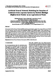
The basic unit of any ANN is the neuron or node (processor). Each node is able to sum many inputs x1, x2,…, x3 whether these inputs are from a database or from other nodes, with each input modified by an adjustable connection weight (Figure 2.2). The sum of these weighted inputs is added to an adjustable threshold for the node and then passed through a modifying (activation) function that determines the final output.

23

Figure 2.2

2.9

Working of node

Feed-forward Network

Though a number of different kinds of ANNs exist, this study will be focusing on feed-forward network. Feed-forward network have been widely used for various tasks, such as pattern recognition, function approximation, dynamical modeling, data mining, and time series forecasting. The training of feed-forward NN is mainly undertaken using the BP-based learning algorithm. A feed-forward NN is a network where the signal is passed from an input layer of neurons through a hidden layer to an output layer of neurons. The function of the hidden layer is to process the information from the input layer. The hidden layer is denoted as hidden because it contains neither input nor output data and the output of the hidden layer generally remains unknown to the user.

Figure 2.3 depicts the feed-forward NN where computation proceeds along the forward direction only. The output obtained from the output neurons constitutes the network output. Each layer will have its own index variable: k for output neurons,

24 j for hidden, and i for input neurons. In a feed-forward network, the input vector, x, is propagated through a weight layer, Wij,

o j = f (net j )

(2.1)

net j = ∑ Wij oi + θ j

(2.2)

o k = f (net k )

(2.3)

net k = ∑ W jk o j +θ k

(2.4)

j

k

where f is an output function (possibly the same as f above in hidden layer).

o k = f (net k )

Wjk

net k = ∑ W jk o j +θ k k

o j = f (net j )

Wij

net j = ∑ Wij oi + θ j j

Figure 2.3

A feed-forward network

25 2.10

Multilayer Perceptron (MLP)

MLP with one hidden layer is one of the most popular types of feed-forward NN. This type of NN is known as a supervised network because it requires a desired output in order to learn. The goal of this type of network is to create a model that correctly maps the input to the output using historical data so that the model can then be used to produce the output when the desired output is unknown. The architecture of MLP is variable but in general will consist of several layers of neurons. The input layer plays no computational role but merely serves to pass the input vector to the network. An MLP may have one or more hidden layers and finally an output layer. MLP is described as being fully-connected, which each neuron connected to every neuron in the next or previous layer. By selecting suitable set of connecting weights and activation functions, it has been shown that MLP can approximate any smooth, measurable function between input and output vectors.

The MLPs consists of a system of simple interconnected neurons as illustrated in Figure 2.4, which a model representing a non-linear is mapping between an input vector and an output vector. The neurons are connected by weights and output signals which are a function of the sum of inputs to the neuron modified by a simple non-linear transfer or activation function. The output of the neuron is scaled by the connecting weight and feed-forward to be an input to the neurons in the next layer of the network. This implies a direction of information processing, hence the MLP is known as feed-forward NN.

For the purposes of this study, the MLP network is also the type of NN most commonly used in time series forecasting (Kaastra and Boyd, 1996). The univarite time series modeling is normally carried out through this NN by using a determined number of the time series lagged terms as inputs and forecasts as outputs. The number of input nodes determines the number of prior time points to be used in each forecast, while the number of output nodes determines the forecast horizon. Thus, a one-step-ahead forecast can be performed through a NN with one output unit and a k-

26 step-ahead forecast can be performed with k output units. Figure 2.4 illustrates an MLP forecasting model in which two past terms in the series used to forecast the value of the series in a one-step-ahead forecast.

Figure 2.4

MLP network for one-step-ahead forecasting based on two lagged

terms

2.11

Backpropagation (BP) Algorithm

The goal of any training algorithm is to find the logical relationship from the given input/output or to reduce the error between the real results and the results obtained with the ANN as small as possible (Zhang, 1992). Any network structure can be trained with BP when desired output patterns exist and each function that has been used to calculate the actual output patterns is differentiable. The BP algorithm is the most computationally straightforward algorithm for training the MLP. As with conventional gradient descent (or ascent), BP works by, for each modifiable weight,

27 calculating the gradient of error (or cost) function with respect to the weight and then adjusting it accordingly.

The input is presented to the network and multiplied by the weights. All the weighted inputs fed to each neuron in the upper layer are summed up, and produced output governed by the following equation. ⎛ ⎞ o k = f (net k ) = f ⎜ ∑ W jk o j + θ k ⎟ ⎝ k ⎠

(2.5)

where ok is the output of neuron k, oj is the output of neuron j at the lower layer, Wjk is the weight between the neuron k and j, netk is the net input feeding to neuron k from the lower layer, θ k is the bias for unit k and f(.) is the activation function of the neuron.

The most frequently used error function to be minimized in BP at the output layer is the mean sum squared error E, defined below

Error, E =

1 (t k − ok )2 ∑ 2 k

(2.6)

where Tk is the target output and ok is the actual outputs of the neuron. According to gradient descent, each weight change in the network should be proportional to the negative gradient of the error with respect to the specific weight.

∆W = −η

∂E ∂W

(2.7)

where η is a constant which represents the learning rate. The learning rate is a parameter to control the rate of convergence. The larger theη , the larger the changes in the weight, thus the faster the desired weight is found. But if η is too large, it may

28 cause oscillations (Danh et al., 1999). The adaptive learning rate is used to reduce the training time (Zhang, 1992).

The derivative of the error function E with respect to weight W in the above equation is proportional to the first derivative of the activation function, i.e.,

∂E ∞f ' (net ) ∂W

(2.8)

The weight change is best understood (using the chain rule) by distinguishing between an error component, − ∂E / ∂net , and ∂net / ∂W . Thus the error for output neurons is

δk = −

∂E ∂o k = (t k − ok ) f ' (o k ) ∂o k ∂net k

(2.9)

and for hidden neurons

⎛ ∂E ∂o

k δ j = −⎜⎜ ⎝ ∂ok ∂net k

∂net k oj

⎞ ∂o j ⎟ = ∑ δ k W jk f ' (o j ) ⎟ ∂net k j ⎠

(2.10)

For a first-order polynomial, ∂net / ∂W equals the input activation. The weight change is then simply

∆W jk = ηδ k o j

(2.11)

∆Wij = ηδ j oi

(2.12)

for output weights, and

for input weights. Rumelhart et al. (1986), proposed an additional term called the momentum which helps to increase the learning rate without leading to oscillations.

29 With the addition of the momentum term and the time subscript, the weight changes become:

∆W jk (n + 1) = ηδ k oi + α∆W jk (n )

(2.13)

∆Wij (n + 1) = ηδ j oi + α∆Wij (n )

(2.14)

for output weights, and

for input weights. Clearly, α (the momentum) is a constant which determines the effect of the past weight changes on the current direction of the movement.

For easier understanding, we have summarized the consecutive steps involved in BP algorithm in the following table.

Table 2.2 : The summarized steps in BP algorithm Step 1 : Obtain a set of training patterns Step 2 : Set up ANN model that consist of number of input neurons, hidden neurons, and output neurons. Step 3 : Set learning rate(η) and momentum rate (α). Step 4 : Initialize all connections ( Wij and Wjk) and bias weights (θk and θj ) to random values. Step 5 : Set the minimum error, E min. Step 6 : Start training by applying input patterns one at a time and propagate through the layers then calculate total error. Step 7 : Backpropagate error through output and hidden layer and adapt weights, Wjk and θk. Step 8 : Backpropagate error through hidden and input layer and adapt weights Wij and θj. Step 9 : Check if Error