Time-series modeling with undecimated fully convolutional neural ...

arXiv:1508.00317v1 [stat.ML] 3 Aug 2015

Time-series modeling with undecimated fully convolutional neural networks

Roni Mittelman [email protected]

Abstract We present a new convolutional neural network-based time-series model. Typical convolutional neural network (CNN) architectures rely on the use of max-pooling operators in between layers, which leads to reduced resolution at the top layers. Instead, in this work we consider a fully convolutional network (FCN) architecture that uses causal filtering operations, and allows for the rate of the output signal to be the same as that of the input signal. We furthermore propose an undecimated version of the FCN, which we refer to as the undecimated fully convolutional neural network (UFCNN), and is motivated by the undecimated wavelet transform. Our experimental results verify that using the undecimated version of the FCN is necessary in order to allow for effective time-series modeling. The UFCNN has several advantages compared to other time-series models such as the recurrent neural network (RNN) and long short-term memory (LSTM), since it does not suffer from either the vanishing or exploding gradients problems, and is therefore easier to train. Convolution operations can also be implemented more efficiently compared to the recursion that is involved in RNN-based models. We evaluate the performance of our model in a synthetic target tracking task using bearing only measurements generated from a state-space model, a probabilistic modeling of polyphonic music sequences problem, and a high frequency trading task using a time-series of ask/bid quotes and their corresponding volumes. Our experimental results using synthetic and real datasets verify the significant advantages of the UFCNN compared to the RNN and LSTM baselines.

1

Introduction

Convolutional neural networks (CNNs) [1] have been successfully used to learn features in a supervised setting, and applied to many different tasks including object recognition [2], pose estimation [3], and semantic segmentation [4]. Common CNN architectures introduce max-pooling operators, which reduce the resolution at the top layers. For tasks such as object recognition, this has the positive property of reducing the sensitivity to small image shifts. However, in many time-series related problems such as nonlinear filtering [5], the input rate has to be identical to the output rate, and therefore the use of the max-pooling operators may pose a serious limitation. In this work, we argue that allowing for the input and output layers of CNNs to maintain the same rate, is critical for many applications involving time-series data. Recently, fully convolutional networks (FCNs), which allow for the input and output signals to have the same dimensions, have been presented in the context of pixel-wise image segmentation [11]. FCNs introduce a wavelettransform-like deconvolution stage, which allows for the input and output lengths to match. In order to apply the FCN for modeling of time-series, we propose an undecimated FCN which takes inspiration from the undecimated wavelet transform [12], and which replaces the max-pooling and interpolation operators with upsampling of the corresponding filters. Our experimental results verify that this modification is necessary in order to allow for effective time-series modeling. We 1

hypothesize that this is due to the translation invariant nature of the undecimated wavelet transform. We refer to our model as the undecimated fully convolutional neural network (UFCNN). A key feature that separates our application of CNNs to time-series from their application to images, is that all the convolution operations are causal. Our UFCNN model offers several advantages compared to time-series models such as the recurrent neural network (RNN) [10] and long short term memory (LSTM) [13], since it does not suffer from either the vanishing or exploding gradients problems [16,23], and is therefore easier to train. It can also be implemented more efficiently, since it only involves convolution operations rather than the recursion that is used in the RNN and LSTM, and is not as straightforward to implement efficiently. An important limitation of our model compared to the RNN and its variants, is that it can only capture dependencies that occur within the overall extent of the filters. Still, this can be accounted for by increasing the number of resolution levels. Since the range of the memory that can be captured grows exponentially with the number of resolution levels, whereas the number of parameters grows only linearly, we argue that our model can in principle account for both long and short-term dependencies. We evaluate the performance of the UFCNN in three tasks. First, we consider a toy target tracking problem of estimating the position coordinates of the target based on bearing measurements. The second task that we consider is the probabilistic modeling of polyphonic music using the dataset that was presented in [22]. Finally, we evaluate the performance of the UFCNN using a high-frequencytrading dataset of ask/bid prices of a security, where we use the UFCNN to learn an investment strategy. Our experimental results show that the UFCNN significantly outperforms the sequential importance sampling (SIS) particle filter (for the the target tracking problem), as well as the RNN and the LSTM baselines. The remainder of this paper is organized as follows. In Section 2 we discuss related works. In section 3 we provide background on the FCNN, and propose our undecimated FCNN. In Section 4 we present the experimental results for the target tracking problem and for the polyphonic music dataset, and in Section 5 we present the experimental results for learning high frequency trading strategies. Section 6 concludes this paper.

2

Related work

CNNs have been introduced in [1], and have recently gained increased popularity due to their remarkable performance in the imagenet large scale image recognition task [2]. Aside from the availability of larger computational resources, the other factors which contributed to the success of CNNs are the use of the rectified linear nonlinearity instead of a sigmoid, and the availability of very large labeled datasets. Recent studies [14,15] have shown that the use of very deep CNN architectures is critical in order to achieve improved classification accuracy. Previous applications of CNNs to time-series signals have typically applied the CNNs to windowed data, therefore producing a single prediction per segment. For example, in [6,7] a CNN was used to predict the phoneme class conditional probability for a segment of raw input signal. In [8] windowed spectrograms were used as the input to a multi-layered convolutional restricted Boltzmann machine, and applied to speaker identification and to audio classification tasks. CNNs have also been used for activity recognition in videos, however, they were mostly used to provide the feature representation for other time-series models [9]. Another deep-learning time-series model is the recurrent neural network (RNN) [10]. RNNs can be trained using the backpropagation-through-time algorithm [10], however, training RNNs can be a difficult task due to the vanishing and exploding gradients problems [16,23]. There have been many works that focussed on extending the modeling capacity of RNNs [22,26], and alleviating the vanishing and exploding gradients problem [25]. The long short term memory (LSTM) [13] addresses the vanishing gradients problem by introducing additional cells that can store data indefinitely. The network can decide when the information in these cells should be remembered or forgotten. A multi-layered LSTM has been recently shown to be very effective in a machine translation task [24]. One time-series model that is particularly relevant to our proposed approach is the clockwork RNN [17], which partitions the hidden layer into different modules that operate at different time-scales. The clockwork RNN architecture can be interpreted as a combination of several RNNs (modules), 2

H1#

G1#

+ H2#

↓2

+

H1#

↓2 ↓2

H3#

G3#

G2#

G0#

↑2 +

↑2

H2#

G2#

+

G1#

G0#

↑2

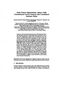
Figure 1: The fully convolutional neural network with 3 resolution levels. The downsampling opH3# G3# layer erators represent the max-pooling layers. The ↓ 2 convolution ↑ 2 G0 is used in order to allow for a negative output. linear units. The (+) symbols represent + H1# The empty rectangles represent rectified G G1# 0# concatenation along the filters axis (“channels” in CAFFE). H2# H1#

+ H3#

G2#

+

G3#

H2#

+ H3#

G1#

G0#

G2#

G3#

Figure 2: The undecimated fully convolutional neural network with 3 resolution levels. Each filter H` or G` represents an upsampled version by a factor of 2`−1 of a base filter, where ` denotes the resolution level. The (+) symbols represent concatenation along the filters axis (“channels” in CAFFE). each operating at a different rate, where there are only inputs from RNNs that operate at lower frequency into RNNs that operate at higher frequency. The RNNs that operate at a lower frequencies are better suited for capturing long-term dependencies, whereas those that operate at higher frequency can capture the short-term dependencies. Each module is therefore analogous to different resolution levels in our UFCNN architecture, which also operate at different time-scales due to the appropriate upsampling of the filter coefficients.

3

Fully convolutional networks for time-series modeling

Our proposed time-series model relies on a CNN that uses causal 1D convolutions. In order to allow for an identical rate both for the input and the output layers, we use a fully convolutional neural network. In this section we first review the fully convolutional neural network, and subsequently present our undecimated version. Our experimental results demonstrate that using such an undecimated version is necessary in order to allow for effective time-series modeling. 3.1

Fully Convolutional Neural Network

A Fully convolutional network (FCN) introduces a decoder stage that is consisted of upsampling, convolution, and rectified linear units layers, to the CNN architecture. The interpolated signal is then combined with the corresponding signal in the encoder which has the same rate. This allows the network to produce an output whose dimensions match the input dimensions. The process is illustrated for the 1D filtering case in Figure 1, where the downsampling operations represent the max-pooling operations. The upsampling operation doubles the rate of the signal by introducing zeros appropriately. A FCN was used in [11] to allow for semantic image segmentation at a finer resolution than that which can be achieved when using standard CNNs. The FCN architecture is in principle very similar to a wavelet transform. As such, it also suffers from the translation variance problem that is associated with the wavelet transform [18]. Due to the use of the decimation operators, a small translation of the signal can lead to very large changes to the 3

representation coefficients. In order to address this issue, we consider using an undecimated FCN that is motivated by the undecimated wavelet transform [12] which is shift-invariant. 3.2

Undecimated fully convolutional neural networks

The undecimated wavelet transform solves the translation variance problem by removing the subsampling and upsampling operators, and instead the filter at the `th resolution level is upsampled by a factor of 2`−1 . Our undecimated FCN therefore uses the same approach, where the filters at the `th resolution level are upsampled by a factor of 2`−1 along the time dimension, and all the other max-pooling and upsampling operators are removed. The UFCNN is illustrated in Figure 2.

4

Experimental results: Bearing only tracking, and probabilistic modeling of polyphonic music

In this section we evaluate the UFCNN in a target tracking task, using bearing only measurements, and using the probabilistic modeling of polyphonic music task that was considered in [22]. We begin by describing the process which we used to generate the synthetic traget data, and then demonstrate that using our undecimated version of the FCN instead of the “vanilla” FCN is necessary in order to allow for effective time-series modeling. Subsequently, we compare the performance of the UFCNN to the RNN and LSTM baselines. In all of our experiments, the filters were initialized by drawing from a zero mean Gaussian, and are learned using stochastic gradient descent with the RMS-prop heuristic [19] for adaptively setting the learning rate. We implemented all the algorithms that are considered here using the CAFFE deep learning framework [20]. 4.1

Generating the target tracking data using a state-space-model

We consider a target that moves in a bounded square, and flips the sign of its appropriate velocity component whenever it reaches the boundary. The observed measurement is the polar angle of the target (with an additive noise component), where the origin is at the center of the square. Specifically, let zt = [xt ; x˙ t ; yt ; y˙ t ], then the state equation takes the form: zt θt

= Ag(zt−1 ) + wt , = arctan (yt /xt ) + νt ,

(1)

where A = [1, 1, 0, 0; 0, 1, 0, 0; 0, 0, 1, 1; 0, 0, 0, 1], wt ∼ N (0, diag([0.5; 0; 0.5; 0]σw )), νt ∼ (0, σν ), and   xt  x˙ , if − D + δ < xt < D − δ, −|x˙ t |, if − D + δ ≤ xt , |x˙ t |, otherwise  g(zt ) =  t  (2) yt y˙ t , if − D + δ < yt < D − δ, −|y˙ t |, if − D + δ ≤ yt , |y˙ t |, otherwise where 2 × D denotes the length of the side of the square, and δ is the radius of the target (which is assumed to be circle shaped). We used the hyperparameters D = 10, δ = 0.3, σw = 0.005, σν = 0.005, for generating the data using the state-space-model. We generated 2000 training sequences, 50 validation sequences, and 50 testing sequences, each of length 5000 time-steps. We used the standard preprocessing approach for CNNs, where the mean that was computed using the training set is subtracted from the input signal at each time-step. 4.2

Evaluating the significance of the undecimated FCN

In order to evaluate the significance of using our undecimated version of the FCN instead of the “vanilla” FCN for time-series modeling, we used the bearings sequence to predict the target’s position at each time-step using the two versions which are illustrated in Figures 1 and 2 respectively. We used a square loss to train the networks. In Tables 1 and 2, we show the mean squared error (MSE) per time-step of the target’s position estimate for the two cases respectively, when varying the number of resolution layers and the number of filters. We used a fixed filter length of 5 for all the 4

filters, and trained each model for 30K iterations, starting with a base learning-rate of 10−3 which was halved after 15K iterations, and a RMS-prop hyper-parameter of 0.9. We trained each model using the training set, and we report the MSE for the validation set (the performance on the testing set is virtually indistinguishable, and therefore we do not report it in Tables 1 and 2). It can be seen that using the undecimated version of the FCN significantly outperforms the standard FCN. We hypothesize that this is due to the shift-invariance property of the undecimated version, and the fact that the same signal rate is maintained throughout the network. # res. / #flt. 1 2 3

100 0.93 0.15 0.06

150 0.86 0.13 0.06

# res. / # flt. 1 2 3

200 0.83 0.13 0.06

Table 1: UFCNN MSE per time-step 4.3

100 0.93 20.14 4 × 108

150 0.86 0.73 1.8

200 0.83 4.86 1.11

Table 2: FCNN MSE per time-step

Comparison to the RNN and LSTM baselines

The baselines to which we compare our model are the RNN and the LSTM. We used the validation set in order to select the hyper-parameters for each model using cross-validation. The MSE per time-step obtained for the testing set using each model is shown in Table 3. It can be seen that the UFCNN outperforms all the other baselines.

MSE

RNN 1.46

LSTM 0.09

UFCNN 0.06

Table 3: Average MSE per time-step for the testing set of the target tracking problem.

4.4

Probabilistic modeling of polyphonic music

Here we evaluate the UFCNN in the task of probabilistic modeling of polyphonic music using the “MUSE” and “NOTTINGHAM” datasets1 [22], which include a partitioning into training, validation, and testing sets. Each sequence represents a time-series with a 88 dimensional binary input vectors, representing different musical notes. We trained the models to predict the input vector at the next time-step, using the cross-entropy loss function. The log-likelihood obtained for the testing set using different algorithms is shown in Table 4, where we used cross-validation to select the hyper-parameters for each model. For the UFCNN, in both dataset cases we used 5 resolution levels with filters of length 2, and 50 filters at each convolution stage. It can be seen that the performance of our RNN implementation is very close to the log-likelihood that was reported in [22] for the same datasets. Our LSTM implementation performs (as expected) better than the RNN, and slightly worse or similarly to the Hessian-Free optimization RNN [25]. Our UFCNN outperforms all these baselines. We note that [22] included comparisons to the RTRBM and RNN-RBM [22], which slightly outperform our UFCNN. We hypothesize that this is due to the fact that restricted Boltzmann machines (RBM) based methods tend to perform better in the scarce data regime that applies to this case, compared to neural network-based methods that operate better when there is abundant data. Dataset MUSE NOTTINGHAM

RNN (Ours) −8.25 −4.62

RNN [22] −8.13 −4.46

LSTM (Ours) −7.5 −3.85

RNN-HF [22] −7.19 −3.89

UFCNN (Ours) -6.67 -3.53

Table 4: Log-likelihood for the “MUSE” and “NOTTINGHAM” datasets.

1

http://www-etud.iro.umontreal.ca/ boulanni/icml2012

5

5

Experimental results: Learning high frequency trading strategies

In this section we consider the dataset of a trading competition is available online2 . The dataset is a time-series in which each time-step includes the best-bid-price and best-ask-price of a security, their corresponding volumes, and several additional indicators that might be useful for predicting future trends in the price of the security. The rate of the time-series in the dataset is about 2-3 samples per second, and the dataset includes a period of one year. We partitioned the data into consecutive training, validation, and testing sets, where we used roughly 8 months for the training set, and 2 months for each of the validation and testing sets. The task which we consider is to learn an investment strategy, i.e. learn a classifier that can predict an action to be executed at every time-step, based solely on past and present observations. The five actions that we consider are: buy at the best-bid-price, sell at the best-bid-price, do nothing, buy at the best-ask-price, and sell at the best-ask-price. The learned strategy should maximize the profit calculated using Algorithm 1, which is based on the market simulator that was provided in the trading competition files. Algorithm 1 accepts as input the time-series of the best ask and bid prices and their corresponding volumes (bidpx, askpx, bidsz, asksz), the actions taken at every time-step, as well as the maximum-position and the cost-per-trade, which were set to 3 and 0.02 respectively in the provided market simulator. 5.1

Learning a trading strategy using a classification approach

Given a time-series, we can find the optimal action to be taken at every time-step in order to maximize the profit by combining the Viterbi algorithm and Algorithm 1. We can then train any timeseries model to predict these actions using a softmax loss layer. A similar classification approach was used in [21] to learn a strategy for playing Atari video games based on offline planning. In Tables 5 and 6 we evaluate the UFCNN when the cost-per-trade parameter is set to 0.02 and 1.0 respectively. We used cross validation to select the hyper-parameters, where for the UFCNN we used 4 resolution levels with filters of length 5, and the number of filters at every convolution stage was 200 and 150 for Tables 5 and 6 respectively. We show the average profit per time-step and the classification accuracy for predicting the optimal decision that is obtained using the Viterbi algorithm, for the testing set. We compare the results obtained using the UFCNN, RNN, the Viterbi algorithm, and a uniformly random strategy. The Viterbi algorithm is aware of the entire time-series and serves here as the unachievable upper bound on the performance. We trained the UFCNN using sequences of length 5000, and we trained the RNN model using sequences of length 200 in order to allow for faster training. It can be seen that the UFCNN is able to achieve significantly larger returns compared to the RNN. Furthermore, it is quite close to the unachievable upper bound that is given by the Viterbi algorithm. For example, the UFCNN’s profit in Table 5 is 50% of the upper bound. We do not show the performance of the LSTM since it consistently diverged during training, which strengthens our claim that the simplified training that is offered by our UFCNN is a major advantage compared to presently available deep-learning-based time-series models. profit/time-step classification accuracy

UFCNN 0.13 0.62

RNN 0.024 0.38

Viterbi (upper-bound) 0.26 1.0

Uniform -0.01 0.2

Table 5: Average profit per time-step, and classification accuracy, for the UFCNN, RNN, Viterbi algorithm (which serves as an upper-bound), and a uniformly random strategy. The cost-per-trade parameter was set to 0.02

6

Conclusions

We presented an undecimated fully convolutional neural network (UFCNN) for time-series modeling. Our model replaces the max-pooling and upsampling operations that are used in the fully convolutional neural network, with upsampling of the filters with a factor that depends on the resolution level. Furthermore, unlike the application of convolutional neural networks to images, we 2

http://www.circulumvite.com/home/trading-competition

6

profit/time-step classification accuracy

UFCNN 0.07 0.68

RNN 0.005 0.69

Viterbi (upper-bound) 0.2 1.0

Uniform -0.01 0.2

Table 6: Average profit per time-step, and classification accuracy, for the UFCNN, RNN, Viterbi algorithm (which serves as an upper-bound), and a uniformly random strategy. The cost-per-trade parameter was set to 1.0

Algorithm 1 Calculate profit for a length T sequence Require: max position, cost per trade, bidpx(t), bidsz(t), askpx(t), asksz(t), action(t) Ensure: pnl← 0, current position← 0, current account← 0 if bidsz(1)+asksz(1)>0 then mktpx1←(bidpx(1)× asksz(1)+askpx(1)× bidsz(1))/(asksz(1)+bidsz(1)) else mktpx1←(bidpx(1)+askpx(1))/2 end if for t ← 1, . . . , T − 1 do mktpx0←mktpx1 if bidsz(t + 1)+asksz(t + 1)>0 then mktpx1←(bidpx(t + 1)× asksz(t + 1)+askpx(t + 1)× bidsz(t + 1))/(asksz(t + 1)+bidsz(t + 1)) else mktpx1←(bidpx(t + 1)+askpx(t + 1))/2 end if pnl←pnl+current position×(mktpx1-mktpx0) if action(t)=Buy@bidpx and current position-max position then current position←current position-1 pnl←pnl+askpx(t)-cost per trade-mktpx1 end if end for return pnl

use causal filtering operations in order to maintain the causality of the model. We demonstrated that our undecimated version of the fully convolutional network is necessary in order to allow for effective time-series modeling. We evaluated our UFCNN in several tasks: bearing only target tracking, probabilistic modeling of polyphonic music, and learning high frequency trading strategies. Our experimental results verify that our model improves over the recurrent neural network (RNN), and long short-term memory (LSTM) baselines. The UFCNN has several additional advantages over RNN-based models, since it does not suffer from the vanishing or exploding gradients problems. It also allows for a very efficient implementation, since it uses convolution operations that can be implemented very efficiently. 7

References

[1] LeCun Y., and Bengio, Y. (1995) Convolutional networks for images, speech, and time-series. In M. A. Arbib, (ed.), The Handbook of Brain Theory and Neural Networks. MIT Press. [2] Krizhevsky, A., Sutskever, I. and Hinton, G. E. (2012) ImageNet Classification with Deep Convolutional Neural Networks. NIPS. [3] Toshev, A., and Szegedy, C. (2014) DeepPose: Human Pose Estimation via Deep Neural Networks. CVPR. [4] Girshick, R., Donahue, J., Darrell, T., Malik J. (2014) Rich feature hierarchies for accurate object detection and semantic segmentation. CVPR. [5] Arulampalam, S. M., Maskell, S., and Gordon, N., (2002) A tutorial on particle filters for online nonlinear/non-Gaussian Bayesian tracking. IEEE Transactions on Signal Proc., Vol. 50, pp. 174–188. [6] Palaz, D., Collobert, R., and Magimai-Dos, M. (2013) Estimating Phoneme Class Conditional Probabilities from Raw Speech Signal using Convolutional Neural Networks. INTERSPEECH. [7] Abdel-Hamid, O., Deng, L., Yu, D., and Jiang, H. (2013) Deep Segmental Neural Networks for Speech Recognition. INTERSPEECH. [8] Lee, H., Largman, Y., Pham, P., and Y. Ng, A. (2009) Unsupervised Feature Learning for Audio Classification using Convolutional Deep Belief Networks. NIPS. [9] Simonyan, K., Zisserman, A., (2014) Two-Stream Convolutional Networks for Action Recognition in Videos. NIPS. [10] Rumelhart, D. E., Hinton, G. E., and Williams, R. J. (1986) Learning representations by back-propagating errors. Nature, 323(6088): pp. 533536. [11] Long, J., Shelhamer, E., and Darrell, T. (2015) Fully Convolutional Networks for Semantic Segmentation. CVPR. [12] Shensa, M. J. (1992) The Discrete Wavelet Transform: Wedding the A Trous and Mallat Algorithms. IEEE Transaction on Signal Processing, Vol. 40, No. 10. [13] Hochreiter, S., and Schmidhuber, J. (1996) Bridging long time lags by weight guessing and long short term memory. Spatiotemporal models in biological and artificial systems. [14] Simonyan, K., and Zisserman, A. (2015) Very Deep Convolutional Networks for Large-Scale Image Recognition. CVPR. [15] Szegedy, C., Liu , W., Jia, Y., Sermanet, P., Reed, S., Anguelov , D., Erhan , D., Vanhoucke, V., and Rabinovich, A. (2015) Going Deeper with Convolutions. CVPR. [16] Pascanu, R., Mikolov, T., and Bengio, Y. (2013) On the difficulty of training recurrent neural networks. ICML. [17] Koutnk, J., Greff, K., Gomez, F., and Schmidhuber, J. (2014) A Clockwork RNN. ICML. [18] Simoncelli, E. P., Freeman, W. T. , Adelson, E. H., and Heeger, D. J. (1992) Shiftable Multi-Scale Transforms. IEEE Trans. Information Theory, Vol. 38, No. 2, pp. 587–607. [19] Hinton, G., Srivastava, N., and Swersky, K., Neural Networks for Machine Learning - lecture 6. Available at http://www.cs.toronto.edu/ tijmen/csc321/slides/lecture slides lec6.pdf [20] Jia, Y., Shelhamer, E., Donahue, J., Karayev, S., Long, J., Girshick, R., Guadarrama, S., and Darrell, T. (2014) Caffe: Convolutional Architecture for Fast Feature Embedding. arXiv preprint arXiv:1408.5093. [21] Guo, X., Singh, S., Lee, H., Lewis, R., and Wang, X. (2014) Deep Learning for Real-Time Atari Game Play Using Offline Monte-Carlo Tree Search Planning. NIPS. [22] Boulanger-Lewandowski, N., Bengio, Y. and Vincent, P. (2012) Modeling Temporal Dependencies in High-Dimensional Sequences: Application to Polyphonic Music Generation and Transcription. ICML. [23] Sutskever, I., Marten, J., Dahl, G., E., and Hinton, G., E, (2013) On the importance of initialization and momentum in deep learning. ICML. [24] Sutskever, I., Vinyals, O., and Le Q., (2014) Sequence to Sequence Learning with Neural Networks. NIPS. [25] Martens, J., and Sutskever, I. (2011) Learning recurrent neural networks with Hessian-Free optimization. ICML.

8

[26] Michalski, V., Memisevic, R., Konda, K. (2014) Modeling deep temporal dependencies with recurrent “grammar cells”. NIPS.

9