526
IEEE TRANSACTIONS ON POWER SYSTEMS, VOL. 16, NO. 3, AUGUST 2001
Time-Varying Contingency Screening for Dynamic Security Assessment Using Intelligent-Systems Techniques Innocent Kamwa, Senior Member, IEEE, Robert Grondin, Senior Member, IEEE, and Lester Loud, Member, IEEE
Abstract—A time-frequency-based approach for contingency severity ranking and rapid stability assessment is described. The aim is to classify correctly all single or multiple contingencies that may result in loss of voltage or frequency stability in the first 20 s following the last disturbing action. We start by selecting a number of strategic monitoring buses where the phasor measurement units are located to capture representative voltage magnitudes and angles during detailed time-domain simulations, which cover special protection systems and on-load tap-changers. The short-time Fourier transform is then dynamically applied to the responses for extracting selected decision features as the simulation time evolves. It is shown that frequency-domain features such as the peak spectral density of the angle, frequency and their dot product evaluated over the grid areas are reliable time-varying stability indicators that can form the basis of an entirely secure classification system able to respond within 2 to 3 s after the last event in the contingency. This allows early termination of about 60% of permanently stable simulations. Fuzzy logic and neural networks are used together to make initial decisions which are then mixed by voting in order to improve the assessment reliability and security at the expense of a reduced yield. The proposed DSA scheme is successfully tested with 1027 contingencies from two widely differing test systems: a 67-bus fictitious system and a 783-bus system in actual use at Hydro-Québec’s operations planning department. Index Terms—Contingency simulation, dynamic security assessment (DSA), dynamic stability, operations planning, phasor measurement unit (PMU), ranking and screening, transient stability, voltage stability.
I. INTRODUCTION
M
ANY utilities in the world are limited with regard to stability in their routine operation. Moreover, it can be safely stated that stability at any utility becomes a limiting factor during cascade events and extreme contingencies. Dynamic security assessment (DSA) is therefore an important operating function, which is currently performed in the back office by operations planners days or hours ahead to specify the conditions under which the power system will be operated with safe stability margins [1]. Effective DSA requires step-by-step time-domain simulation, which is both computationally intensive and time-consuming. That is the main reason why DSA is still not widely available on-line in standard EMS packages [2]–[4]. However, extensive research is underway throughout Manuscript received December 5, 2000. The authors are with Hydro-Quebec/IREQ, Power System Analysis, Operation and Control, 1800 Lionel-Boulet, Varennes (Qc) Canada, J3X 1S1 (e-mail:
[email protected]). Publisher Item Identifier S 0885-8950(01)06076-X.
the world in order to make DSA faster and suitable for on-line use [1]–[21]. We can isolate two main trends in this search for faster DSA. The first relies on energy functions or pattern recognition techniques to rapidly rank and screen out nonsevere contingencies, leaving only a few severe cases for more time-consuming analysis [5]–[8]. The second approach, on the other hand, is an attempt to speed up step-by-step detailed simulations of all contingencies using multi-processor computations, for instance [1], [4]. It is also possible to derive a third axis of research by combining the first two [9], [10]. Historically, transient energy function (TEF) based methods have been aimed at direct stability assessment without time-domain simulation [5]. However, much better results have recently been obtained with hybrid methods, as they keep the time-domain simulation and all detailed models [11]–[13]. Energy function computations are based on many simplifying assumptions which, depending on the operating conditions, are not always true. Also, they address only part of the problem (first swing stability and steady conditions). It is very difficult, if not impossible, to assess cascade effects and fast voltage and multi-swing instability using such tools [3]. Recognizing these limitations, some authors are proposing that detailed simulation of all contingencies be maintained to be able to cover all types of dynamic instabilities [1], [3]. The challenge then is to determine intelligent early-termination criteria, allowing simulation of stable cases to be aborted as soon as possible [9], [10]. This should make it possible to achieve the analytical accuracy of time-domain simulations of the full system while reducing the computational burden to acceptable levels for on-line implementation on a multi-processor platform. Early-termination criteria for time-domain simulations can be defined on the basis of coherency, transient energy conversion between kinetic energy and potential energy, and the dot product of system variables. However, only this last criterion has been tested so far [9], [10]. In this paper, we will develop termination criteria in the frequency domain while using detailed time domain-simulation to determine the stability status of a contingency. This choice is motivated by the greater reliability of spectral quantities as time-varying energy and stability indicators [15], [26]. Using the short-time Fourier transform, we show that this approach can be implemented in such a way that the stability indicator is a continuous variable which builds up as information about the stable/unstable status of the contingency accumulates during the simulation. The strength of this approach is that there is no
0885–8950/01$10.00 © 2001 IEEE
KAMWA et al.: TIME-VARYING CONTINGENCY SCREENING FOR DSA USING INTELLIGENT-SYSTEMS TECHNIQUES
527
limitation in the modeling or the type of instability that can be considered. The pitfall is that we have to agree to simulate the system for a few seconds before deciding about its status. Moreover, there is no stability margin or transfer limit available at the end of the process: it needs to be determined separately, using the approaches in [3], [15], for instance. The paper proceeds as follows. In Section II, the test systems used in the study are described, together with the approach used for sampling the power system responses. In Section III, frequency-domain severity indices are defined using the average frequency and voltage of various areas in the grid. Section IV illustrates some interesting features of these indices. Contingency screening is performed in Section V using fuzzy logic, neural networks and a hybrid system combining the two. Section VI reports on test results obtained by applying the proposed concepts to two test systems with a total of 778 stable and 249 unstable single and multiple contingencies. Conclusions are drawn in Section VII. II. MONITORING SYSTEM DYNAMICS USING PHASOR MEASUREMENT CONCEPTS Effective assessment of the dynamic performance of the power system requires wide-area information from properly disseminated phasor measurement units (PMU) [16], [22], [27]. However, to maximize the information content of the captured signals, the sensors should be located appropriately, with due account given to the structural properties underlying the given system [20], [25]. Similar concerns apply to the location of remote measurements for secondary voltage control or static state estimation [23]. In any case, optimum sensor location aims at maximizing the overall sensor response to system disturbance while minimizing the correlation among sensor outputs, so as to minimize the redundant information provided by multiple sensors [24]. The sensor responses of interest are the bus voltage and frequency coherency indices that are estimated by statistical sampling of power system response signals obtained from a transient-stability program [20]. To illustrate this monitoring approach at the core of the proposed DSA engine, we will consider two test systems: a 783-bus Hydro-Québec system and a 67-bus fictitious system, shown in Figs. 1 and 2, respectively. The Hydro-Québec test system is an actual model of the grid used for operations planning at TransÉnergie, the province of Québec’s ISO. The peak winter load is normally 35 000 MW. Other characteristics of the study are: 1072 lines and 130 generators and 9 synchronous condensers modeled in detail. A simplified representation of three HVDCs is also included while on-load tap changers, and the 10 SVCs have detailed representations. Hydro-Québec’s defense plan against extreme contingencies [28] is also represented in detail. Loads are represented by a nonlinear exponential model. The artificial test system was built from scratch to illustrate dynamic interactions in multi-area power systems. It consists of two well-defined cells replicated a number of times with different dynamic data and interconnected using tie lines of different power transfer capability. The overall network has 67 buses, 23 machines modeled in detail and about 7000 MW
Fig. 1. Hydro-Québec test system.
Fig. 2. Artificial test system.
of nonlinear loads spread over nine geographical areas, which closely overlap the underlying electrically coherent areas. Dynamic performance monitoring of grid during disturbances is based on observations taken by phasor measurement units at suitably located buses. Figs. 2 and 3 illustrate the bus locations for the two networks under study. The placement was achieved using unpublished methods [31], which are nonetheless very similar to those described in [20] and [23]. The first step is to divide the network into a number of electrically
528
IEEE TRANSACTIONS ON POWER SYSTEMS, VOL. 16, NO. 3, AUGUST 2001
Fig. 3. Artificial test system: 63 PMUs in a 783-bus system.
coherent areas following weak inter-tie lines or systematically identified stability boundaries [20], [25]. For instance, applying fuzzy clustering techniques to a large number of response signals to small and large disturbances, it was possible to identify about nine areas in the Hydro-Québec network which are interlinked by a number of 315- and 735-kV lines. In the same way, it was possible to confirm that the artificial test system consisted of nine interconnected coherent areas, linked together by a number of 120- and 230-kV lines. The next step in optimum PMU placement is to assign mandatory measurement units at the boundary of the areas [25], since every tie line should be monitored constantly, not only for security reasons but also for metering and routine operation. Then a sequential addition algorithm [23], [24] is applied to the same database in order to expand the number of PMUs allocated for monitoring, while maximizing the amount of information added by each new PMU. At some point during this sequential addition, the incremental amount of information, as measured using an entropy-based criterion, becomes very small and the process stops, giving a minimum number of PMUs that allows good coverage of the dynamic response data involved in the database. During the simulation of a given contingency in the stability program, only the buses with a PMU will be monitored. The corresponding voltage and angle will be sampled, typically with a variable sampling rate ranging from 1 point per cycle at fault inception to 6 points per cycle, 600 cycles after the fault. This data is then stored in the files in MATLAB format for further processing. III. SEVERITY INDICES A. PMU-Based Center of Inertia (COI) Signals The severity indices are defined with respect to Figs. 3 and 4 by associating with each area an equivalent inertia representing the total inertia of the generation located in that area. Table I summarizes this data for the two systems under study. Assuming that each area is coherent following a disturbance, it is reasonable to assimilate its behavior to that of a single large
Fig. 4. Artificial test system: 38 PMUs in a 67-bus system. In parentheses: number of buses in the area. TABLE I CUMULATIVE AREA INERTIA AND GENERATION
machine with the same inertia and generation. Although this assumption is not perfect, it offers a straightforward means of deriving the center of inertia (COI), which is a very useful information for tracking the stability of the interconnected areas. Before defining the COI quantities, we first need to introduce the area pilot angle concept. For area number , equipped with PMUs, the area angle is the average angle through all measurements: (1) Then assuming a total of areas in the network, we can define the COI of the system as follows: (2) is the total inertia of the grid and is the th area where inertia, as given in Table I. From here on, the area pilot angle and frequency expressed in the COI frame are given by: (3)
KAMWA et al.: TIME-VARYING CONTINGENCY SCREENING FOR DSA USING INTELLIGENT-SYSTEMS TECHNIQUES
529
where is the spectral line index, a discrete-time index and the sampling period of the data sequence of length . It is important to recall that the above definition of the DFT implicitly assumes the periodicity of . Based on (6), an estimate of of is given by: the power spectral density (7) is the acceleration power of the On the other hand, if equivalent machine, which mimics the behavior of the th area, then its swing equation is: (8) Integration of (8) over a horizon of N samples corresponding to is: the interval Fig. 5. Nonlinear filter for determining time-domain coherency-based severity indices (N is the time horizon of the index in samples).
(9) In the same way, area pilot acceleration can be defined in the . Another useful COI frame as the second derivative of quantity in assessing the contingency severity is the dot product of the frequency and the angle: (4) is the speed deviation in the COI frame and is the area pilot-angle deviation from its post-fault value immediately at the clearing instant. Fig. 5 shows a filter which allows computing a family of severity indices based on the coherency concept:
where
(5) where is the number of areas and is the contingency severity ), frequency ( index associated at time to the angle ( ), acceleration ( or dot-product ( ). Hence, an can be computed sample by sample, angle severity index starting at fault clearing, thus yielding a time-varying severity index based on the maximum angle difference between areas over a sliding window of samples. B. Motivation for the Frequency-Domain Perspective It is well known that sequential spectral monitoring of electromechanical oscillations provides important information about the behavior characteristics of system transients. The reason is essentially that the spectral density of the oscillatory signal responses is closely related to the excess kinetic energy injected into the system by the fault. Let us consider more specifically from its the deviation of the th area pilot-frequency signal . The discrete Fourier immediate post-fault value, transform (DFT) can be used to convert this time-domain signal into the frequency domain:
(6)
is the base frequency of the equivalent machine. The where accumulated integral in (9) represents the excess kinetic by the th area equivalent machine during the time interval . Computing the spectral density of , based on the DFT definition in (6), yields the frequency-domain kinetic energy [26]: (10) which is proportional to the spectral density of . This allows ) as an indirect meaus to use the spectral density of ( surement of the excess kinetic energy injected by the fault into the system. More generally, this approach can be extended to other relevant signals, such as the angle ( ), the acceleration ( ), and the dot product ( ). In reference [15], the spectrum of the voltage is also effectively used as a measure of the excess energy injected into the system, defined as the integral of the square voltage deviation from its reference value. C. Fast Computation of Frequency-Domain Severity Indices Computing the spectral density of the various signals resulting from a contingency simulation is complicated by the fact that the stability signals are non stationary and contain time-varying DC components and offsets resulting from the difference between the pre-fault and post-fault steady-state values. A widely known cure to this problem is the short-time Fourier transform (STFT), which is a time-frequency analysis scheme [29] specifically conceived for non parametric detection of changing spectra: speech, machine vibrations, etc. The starting point of the STFT is a low-pass filter with a finite impulse response (FIR), which is essentially the spectral windows referred to previously. Let us denote its impulse response . Suppose we are interested in knowing the amby plitude and phase of one spectral component, , only. This goal can be achieved using the scheme in Fig. 6(a). The incoming . Hence, this spectral signal is mixed with the reference line is shifted to DC, where it is collected by low-pass filtering. From input to output, the processor thus acts like a bandpass filter with a decimation stage for data compression purposes.
530
IEEE TRANSACTIONS ON POWER SYSTEMS, VOL. 16, NO. 3, AUGUST 2001
The second processing step then computes the spectral density of the input signal with a prescribed decimation factor, i.e., a spectral estimate is provided only every input samples (see Fig. 6). For each area, the peak of the PSD is taken over the spectral lines and, finally, the largest value among the areas is selected as the frequency-domain severity index. Hence, can be computed sample by a STFT-based severity index sample, starting at fault clearing, thus yielding a time-varying frequency-domain severity index proportional to the excess kinetic energy injected by the fault in the most disturbed area. This index is refreshed at a prescribed sampling rate of one sample input samples, allowing a severity assessment to be made per on a time-varying basis as the system behavior evolves. IV. ILLUSTRATION OF SEVERITY INDICES
Fig. 6. Multi-rate filter bank approach to spectral analysis (m and discrete-time indices while l is the spectral line index.
n
are
Fig. 7. Computation of frequency-domain severity indices.
The STFT only generalizes this simple phasor demodulation process to N spectral lines simultaneously, not by using a single bandpass filter but a bank of N such filters [Fig. 6(b)]. For a sampling frequency , it is convenient to space the center frequencies of the bandpass filters uniformly by a bin frequency: . Uniform spacing makes it feasible to implement the computational scheme in Fig. 1(b) using the fast Fourier transform (FFT) algorithm [29]. Based on this very efficient computational structure, Fig. 7 shows a block diagram for computing frequency-domain severity indices. At the entry, we have the selected area pilot ), frequency ( ), accelersignal such as the angle ( or dot product ( ). Since its energy makes ation ( sense in assessing the contingency security, we can also choose the area pilot-voltage deviation as an input to Fig. 7: (11)
For the remainder of the study, 150 contingencies were defined for the fictitious test system and 877 contingencies for the Hydro-Québec test system. On the fictitious network, three generation-load dispatch scenarios were considered and 50 contingencies applied to each of them. Most of these contingencies were typical 6-cycle three-phase faults at transmission buses followed by a single-line outage, although the database was enlarged by a number of cascade events, such as generation or load shedding after a double line outage. On the Hydro-Québec system, 10 scenarios of load-generation dispatch corresponding to typical winter or summer load patterns from 1996 to 2001 were considered, including or not Hydro-Québecs defense plan against extreme contingencies [28]. Seventy-seven contingencies were then obtained from the operations planning department where they are routinely used for making provisional dynamic security assessments several days ahead. They included single- and three-phase faults at all 735-kV buses with a single- or double-line outage and, in some situations, islanding of particular regions as required by the practicalities of network operation. In addition to these 77 carefully selected cases, about 10 multiple-contingency cases were generated artificially, by cascading normal faults with HVDC faults or remote shedding of generation and load. The resulting 1027 stability simulations were performed in batch using a UNIX script [1], [19]. Then, the spectral analysis of the database was automated using MATLAB scripts. For that purpose, a custom STFT program was implemented with the , , Hz and following parameters: . The time response of this PSD estimator is therefore s, which means that practical decisions based on it had to be delayed for about 2 s after fault clearing. Clearly, this approach should not be confused with the energy function approach, which is prepared to classify the case at the faultclearing time. For example, a 0.5-s window after fault clearing was used by Fu and Bose in their coherency-based approach [14]. Fig. 8 shows the Hydro-Québec responses to a typical stable fault. The top curve displays the angle shift of each area in the COI frame while the bottom curve portrays the peak of the frequency PSD for each area. The maximum angle shift is small (less than 5 ) and this is translated in the frequency-domain kinetic energy by a corresponding small peak occurring at about
KAMWA et al.: TIME-VARYING CONTINGENCY SCREENING FOR DSA USING INTELLIGENT-SYSTEMS TECHNIQUES
531
(a) Transient instability Fig. 8. Sample stable contingency. Top: time-domain; Bottom: frequencydomain.
s. The kinetic energy subsequently fades away, confirming that the post-fault system is stable. In Fig. 9, three unstable cases are represented using the same picture arrangement. The first case [Fig. 9(a)] is an inertial transient-instability phenomenon while the case below is a post-inertial dynamic instability [Fig. 9(b)]. Fig. 9(c) corresponds to a post-inertial voltage collapse. Overall, in the time domain, the angle shift information is not very expressive about the contingency status (stable/unstable), since the maximum angle, even just before system collapse, is in the range of 20 to 80 and therefore very far from the critical 180 angle. However, the peak of frequency PSD is higher than 0.1 when the system is unstable and less than 0.1 when it is stable. The voltage collapse case is not as easy to classify using frequency PSD only, and it is natural to seek more information, such as the PSD of pilot voltage deviation. This gives rise to a multi-criteria decision, as suggested elsewhere [6], [14], [17].
(b) Dynamic instability
V. CONTINGENCY SCREENING A. Frequency-Domain Features for Classification To assess the contingency status, 28 more-specific criteria were defined in the frequency domain, based on the generic severity indices defined in the previous section. To this end, a reference ( ) and decision time ( ) are first selected. The first set of criteria is the severity indices at these times: and
(12)
The next set of features comprises the maximum values of the : severity indices over (13) A new set can be defined as the ratio of features (12) and (13): (14)
(c) Dynamic instability Fig. 9. Sample unstable contingencies. Top: time-domain; Bottom: frequency-domain.
is normally much less than 1 for stable cases but The feature should be close to 1 for unstable cases. In addition to the above
20 features, eight others were generated from the COI angle and and frequency. The peak of the PSD of these two signals
532
IEEE TRANSACTIONS ON POWER SYSTEMS, VOL. 16, NO. 3, AUGUST 2001
Fig. 11. Fuzzyfication of the decision features.
Fig. 10. Sample features for Hydro-Québec system (T = 1:75 s and T = 2:25 s).
were computed and formulas (12)–(14) applied to them, yielding eight different features. Such COI-related indices are useful for assessing large system-wide slow motions, such as the 0.05-Hz mode present in both the Hydro-Québec and the fictitious test systems. Fig. 10 illustrates some of the adopted features for about 105 contingencies, on a logarithmic scale. Since abnormally large values correspond to unstable contingencies, it is clear that most of the contingencies are stable. For illustration, time- and frequency-domain signals associated to the stable contingency no. 980 are shown in Fig. 8. B. Fuzzy Classification Fuzzy classification applies fuzzy reasoning to a subset of features to decide at time , whether a contingency is permanently stable. To simplify the reasoning and make it as transparent as possible, only four features are used: and
(15)
Each input feature is first normalized using the natural logarithm function. Then it is fuzzyfied by assigning them three membership functions (Fig. 11): 1 (stable), 0 (undecided) and 1 (unstable). The threshold values in Fig. 11 are chosen such
Fig. 12.
Fuzzy decision system for classifying the severity of contingencies.
that, if the feature value is below, the system is stable with a probability of 1. In the same way, for a feature value greater than, the contingency is definitely unstable. However, for other feature values, the system is stable or unstable with a probability value less than one, which means than additional information is needed to reach certainty. The overall structure of the fuzzy decision system is shown in Fig. 12. Its output is a severity index with values in the range, where 1 means a very stable, and 1 a very unstable, contingency. A value around zero means that and more information the case is undecided at decision time or time is required to achieve a crisp decision. Therefore, the output of the fuzzy classifier is much like a continuous-variable severity grade of the contingency. For fuzzy inference, the following set of five rules was defined heuristically, in terms of the various feature classes: is (0), then severity is (0) 1) If is ( 1) and is ( 1), then severity is 2) If ( 1) is (1) and is (1), then severity is (1) 3) If is (0) and is ( 1), then severity is (0) 4) If is (1) and is (1), then severity is (1). 5) If Despite its simplicity, parsimony and transparency, this rule set was quite successful, as highlighted in Section VI.
KAMWA et al.: TIME-VARYING CONTINGENCY SCREENING FOR DSA USING INTELLIGENT-SYSTEMS TECHNIQUES
Fig. 13.
533
Selected neural network architecture. Fig. 14.
C. Neural Network Classification The selected architecture (Fig. 13) consisted of two sigmoid neurons in the hidden layer and one linear neuron at the output, which should give 1 for stable and 1 for unstable contingencies. All 28 features previously defined are used simultaneously at the network input, after natural logarithm normalization. The training of the neural network is based on the 1027 contingencies associated with the two test systems. To increase the number of patterns and randomize the feature input values, the decision time was varied in 0.5-s steps, under a fixed reference : time
This yields a total of 5135 patterns, which were split in two: – A training set with 2835 patterns, corresponding to and – A testing set with 2300 patterns corresponding to and . The training was performed in the MATLAB neural network toolbox [30]. The 2835 patterns were shuffled a few dozen of times before training, to enhance randomness of the data and minimize sequential bias effect. After the data was shuffled, it was again divided into two equal sets: one for training, the other for verification. During each learning period, two optimizations were performed in sequence: – The first started from random parameters and trained the neural network using a Levenbert–Marquartd learning method until the verification error started to rise instead of decreasing. This was to prevent overtraining of the initial network. – The second optimization stage used a BFGS-based quasi-Newton learning method, starting from the previous stage solution. After each training cycle, the neural network parameters were saved, as well as the total rms error over the 2835 training patterns. When a new model has an rms error bigger than that of the previous best model, it is discarded; if not, it replaces the previous best model. This process was repeated about 1000 times before convergence was decided, following 20 optimization cycles without changing the best previous model. D. Intelligent-System-Based Hybrid Classification The output variables of the previous fuzzy logic and neural network-based decision systems are continuous variables in the range [ 1, 1], which means that a certain post-processing is
Hybrid intelligent decision system.
required to reach a final decision, based for instance on selecting a suitable threshold for a binary test. The rules used in the postprocessing are given below: Neural network: If (output 0.75) then UNSTABLE contingency 0.75) then STABLE contingency Else If (output Else UNDECIDED contingency Fuzzy logic system: If (output 0.35) then UNSTABLE contingency 0.02) then STABLE contingenElse If (output cyElse UNDECIDED contingency The thresholds in these binary tests were chosen empirically in order to fit the Hydro-Québec and fictitious test systems simultaneously. Since these two systems are quite different in their behavior, it is believed that the proposed thresholds are representative of a large variety of power system con-figurations. In order to take advantage of both the fuzzy logic and a neural network to achieve a more reliable and secure classification, the results from the two blocks are passed through an AND gate to provide the final decision according to Fig. 14. For a contingency to be ultimately declared stable (unstable), it should be stable (unstable) according to the two inference engines simultaneously. Any contingency that is neither stable nor unstable after the hybrid processing remains undecided. In general, the latter are severe contingencies requiring detailed simulations on a time frame greater than the assumed decision time . VI. TEST RESULTS The 1027 contingencies in the database are divided into 778 stable cases and 249 unstable cases, of which 132 experienced instability within 2 s of simulation. The objective of the classification is to avoid a full simulation of the 778 stable contingencies, in order to save computation time. A case is stable if it can be simulated completely by the stability program for 20 s. The stopping criterion in this program is a more than 200 angle shift between any two machines. However, for the purpose of classification in this study, we consider it realistic to declare any case involving islanding of a part of the network as unstable. The performance of the classification will now be assessed using three criteria: 1) False-dismissals rate: (number of cases declared stable by the classifier while actually unstable)/1027. 2) False-alarms rate: (number of cases declared unstable by the classifier while actually stable)/1027. 3) Classification yield: (number of cases declared stable by the classifier)/(number of stable cases in the database).
534
IEEE TRANSACTIONS ON POWER SYSTEMS, VOL. 16, NO. 3, AUGUST 2001
TABLE II CLASSIFICATION ASSESSMENT FOR THE TWO TEST SYSTEMS
The first criterion is a security measure: it is required that this rate be 0 or very low (less than 0.5%). The next criterion is a reliability measure. For this application it is not as critical as the previous one, although it will adversely impact the effectiveness of the contingency filtering. The last criterion measures the yield of the filtering in terms of how many stable and nonsevere contingencies were actually screened out. Table II summarizes the classification results in terms of these performance measures. To introduce some randomness in this assessment, classification results are reported for six decision time instants between 2.25 and 4.5 s, which means that no stable case can be singled out before 2.25 s of detailed simulation. As mentioned previously, this is one limitation of the proposed approach, but it is a cost readily paid for good coverage of all type of contingencies (including cascade events with protection system operation), and all types of transient and dynamic instability phenomena. A. Fuzzy Classification Looking at the fuzzy-logic results first, it is observed that for a fixed reference time as used in our work, this approach is sensitive to the decision time. At first, the yield is 63.6% s. At the same time, howbut it rises to 89.2% by ever, the false-dismissals rate is getting worse, rising from 0% to 1.2%. It seems that the best decisions were at 3 s, with 0.8% false alarms and no false dismissals. This does not surprise us, since the configuration of the membership function and decision thresholds were decided assuming this particular decision time. Interestingly, even though the classification is best at 3 s it is not so bad at other times, thus conforming the robustness of the classification. To fully appreciate this success, may we
Fig. 15.
Fuzzy severity grades on the scale [-1, 1].
emphasize that we are using no more than five features and five rules for this purpose. Fig. 15 illustrates the severity grade of all contingencies, on a [ 1, 1] scale, according to the fuzzy-logic reasoning. The first plot at the top corresponds to the fictitious system. The contingency severity tends to be high here because it is a weak system with only a few PSSs. The three other plots in the figure are associated with 877 Hydro-Québec contingencies. This time, the severity grade is more evenly spread over the [ 1, 1] range. The grades around zero correspond to severe disturbances, most of which are either voltage unstable or small-signal unstable, or involve large post-contingency offsets in frequency or angles. B. Neural-Network Classification The neural-network results are even more impressive than those obtained with the fuzzy logic. It is possible in this approach to abort the simulation of about 83.8% of the stable cases present in the database after only 2.25 s. In addition, this is achieved with rather low false alarms and dismissals rates of 1 and 0.1% respectively. Since the false-alarm rate is higher, it is interesting to get a closer look at a few contingencies in this case. It is found that most of them are from the fictitious system, which is a weak system allowing for large swings during mild disturbances.
KAMWA et al.: TIME-VARYING CONTINGENCY SCREENING FOR DSA USING INTELLIGENT-SYSTEMS TECHNIQUES
(a) False alarm
(b) False dismissal Fig. 16. Two cases misclassified by the neural network at Td = 3 s. Top: time-domain; Bottom: frequency-domain.
Fig. 16 shows the signals associated with one false alarm and one false dismissal generated by the neural net on this fictitious system at 3 s. It appears that the false-alarm case is very severe albeit stable within the 20-s simulation frame, while the falsedismissal case is not transiently unstable, but unstable only after sustained small-signal oscillations. We believe that fast recognition of the latter type of instability is out of reach of currently used transient-energy functions-based screening methods. C. Hybrid Decision System Since the neural network and fuzzy logic suffer a few falsedismissal hits not occurring in the same cases, it was possible to completely eliminate this problem with a hybrid voting decision system. However, using an AND gate as in Fig. 14 guarantees 100% security at all decision times at the expense of lower yields, compared to fuzzy-logic and neural-network decision systems. The optimum yield with respect to the computational time saving occurs at 3 s and amounts to 71%. One false
535
alarm is still present, due to the fact that the severity of certain so-called stable contingencies is rather high, especially for the fictitious test system. Two early termination criteria were proposed previously [9], [10]. They both used dot products similar to (4) to determine, from their sign changes during simulation, the earliest time it can be concluded that the case will remain permanently stable for future simulation steps. Such a scheme allowed for an average 30–50% time saving in [10] and up to 100% in [9]. However, yield comparisons are complicated by the fact that some authors focus on inertial instabilities while others also consider post-inertial instabilities. Sometimes the number of unstable cases (2, in [10]) is so small that the false-dismissals rate becomes statistically insignificant, while at other times the total number of cases may be too few for the yield to be conclusive (30, in [9]). In addition, only a few authors [1], [3], [4] attempt to cover any instability event that may occur in the normal simulation time frame of 20 s, irrespective of its underlying mechanism. This is an important consideration, however, given that power system responses in the case of multiple contingencies and cascade events with concomitant special protection reactions are not easy to predict a long time ahead, which makes difficult a reliable decision about the stable/unstable status of a case immediately at fault clearing without a few seconds of simulation. As shown by the hybrid classification results in this paper, detailed analysis of the characteristic signatures in these initial few seconds of data can help to differentiate permanently stable cases from severe cases, which may become unstable later during the simulation. In addition, since this assessment is time-varying, decision can be delayed as necessary until sufficient information is captured in the features to allow a reliable decision. This way, the simulation program is able to adapt the simulation duration to the severity of the case. VII. CONCLUSION This paper proposed a novel approach to DSA speed-up using frequency-domain severity indices that are computed dynamically with the help of the short-term Fourier transform. The basic idea is to extract characteristic features from these severity indices and introduce them into a fuzzy-logic and neural-network decision system, which then provides a more appealing indication of the stable/unstable status of the contingency. In both cases, the output is a continuous decision variable on the scale [ 1, 1], which can be viewed as a convenient severity grade allowing the contingencies to be ranked. Although the decision has to be delayed for about 2 s after the last disturbing action in the contingency, it turns out to be highly reliable and 100% secure, if the fuzzy-logic and neural-network conclusions are combined through a logical AND. For a network with a set of nonlinear models and special protection systems as extensive and diversified as Hydro-Québec’s, this conservative DSA approach without model simplification and including cascade events of any type seems well-suited and able to screen out about 60% of the stable cases without any false dismissals after just 2 to 3 s of detailed simulations.
536
IEEE TRANSACTIONS ON POWER SYSTEMS, VOL. 16, NO. 3, AUGUST 2001
REFERENCES [1] L. Riverin and A. Valette, “Automation of security assessment for hydroQuebec’s power system in short-term and real time modes,” in CIGRÉ, Paris, 1998, paper 39-103. [2] Y. Mansour, E. Vaahedi, A. Y. Chang, B. R. Corns, B. W. Garett, K. Demaree, T. Athay, and K. Cheung, “B.C. Hydro’s on-line transient stability assessment (TSA)—Model development, analysis, and post-processing,” IEEE Trans. Power Systems, vol. PWRS-10, no. 1, pp. 241–253, Feb. 1995. [3] J. L. Jardim, C. A. da Neto, A. P. A. da Silva, D. M. Falcao, A. C. Z. de Souza, C. L. T. Borges, and G. N. Taranto, “A unified online security assessment system,” in CIGRÉ, Paris, 2000, paper 38-102. [4] V. Chadalavada, V. Vittal, G. C. Ejebe, G. D. Irisarri, J. Tong, G. Pieper, and M. McMullen, “An on-line contingency filtering scheme for dynamic security assessment,” IEEE Trans. Power Systems, vol. PWRS-12, no. 1, pp. 153–161, Feb. 1997. [5] H. D. Chiang, C. S. Wang, and H. Li, “Development of BCU classifiers for on-line dynamic contingency screening of electric power systems,” IEEE Trans. Power Systems, vol. PWRS-14, no. 2, pp. 660–666, May 1999. [6] V. Brandwajn, A. B. R. Kumar, A. Ipakchi, A. Bose, and S. D. Kuo, “Severity indices for contingency screening in dynamic security assessment,” IEEE Trans. Power Systems, vol. PWRS-12, no. 3, pp. 1136–1142, Aug. 1997. [7] Y. Mansour, E. Vaahedi, M. A. El-Sharkawi, A. Y. Chang, B. R. Corns, and J. Tamby, “Large scale security screening and ranking using neural networks,” IEEE Trans. Power Systems, vol. PWRS-12, no. 2, pp. 954–960, May 1997. [8] F. Aboytes and R. Ramirez, “Transient stability assessment in longitudinal power systems using artificial neural network,” IEEE Trans. Power Systems, vol. PWRS-11, no. 4, pp. 2003–2010, Nov. 1996. [9] G. C. Ejebe, C. Jing, J. G. Waight, V. Vittal, G. Pieper, F. Jamshidian, D. Sobajic, and P. Hirsch, “On-line dynamic security assessment: Transient energy based screening and monitoring for stability limits,” in 1997 IEEE/PES Summer Meeting, Berlin, Germany. [10] M. La Scala, G. Lorusso, R. Sbrizzai, and M. Trovato, “A qualitative approach to transient stability analysis,” IEEE Trans. Power Systems, vol. PWRS-11, no. 4, pp. 1996–2002, Nov. 1996. [11] E. Vaahedi, Y. Mansour, and E. K. Tse, “A general purpose method for on-line dynamic security assessment,” IEEE Trans. Power Systems, vol. PWRS-10, no. 1, pp. 241–253, Feb. 1995. [12] K. Morison, H. Hamadanizadeh, and L. Wang, “Dynamic security assessment tools,” in Proc. of the 1999 IEEE/PES Summer Meeting, Edmonton, Alberta, Canada, pp. 282–286. [13] R. Aresi, B. Delfino, G. B. Denegri, S. Massucco, and A. Morini, “A combined ANN/simulation tool for electric power system dynamic security assessment,” in Proc. 1999 IEEE/PES Summer Meeting, Edmonton, Alberta, Canada, pp. 1303–1309. [14] C. Fu and A. Bose, “Contingency ranking based on severity indices in dynamic security analysis,” IEEE Trans. Power Systems, vol. PWRS-14, no. 3, pp. 980–986, Aug. 1999. [15] R. J. Marceau and S. Soumare, “A unified approach for estimating transient and long-term stability transfer limits,” IEEE Trans. Power Systems, vol. PWRS-14, no. 2, pp. 693–701, May 1999. [16] C. W. Liu, M. C. Su, S. S. Tsay, and Y. J. Wang, “Application of a novel fuzzy neural network to real-time transient stability swings prediction based on synchronized phasor measurements,” IEEE Trans. on Power Systems, vol. PWRS-14, no. 2, pp. 685–692, May 1999. [17] A. Bose, W. Li, M. La Scala, and E. De Tuglie, “On-line contingency screening and remedial action for dynamic security analysis,” in CIGRÉ, Paris, 1998, paper 39-113. [18] L. Wehenkel, I. Houben, M. Pavella, L. Riverin, and G. Versailles, “Automatic learning approaches for on-line transient stability preventive control of the Hydro-Québec system, Parts I and II,” in Proc. 1995 IFAC Sympo. on Control of Power Systems and Power Plants (SIPOWER’95), pp. 231–242.
[19] J. D. McCalley, S. Wang, R. T. Treinen, and A. D. Papalexopoulos, “Security boundary visualization for systems operation,” IEEE Trans. Power Systems, vol. PWRS-12, no. 2, pp. 940–947, May 1997. [20] L. Wehenkel, “A statistical approach to the identification of electrical regions in power systems,” in Proc. 1995 Power Tech Conf., Stockholm, June 18–22, 1995, pp. 530–535. [21] A. L. Bettiol, L. Wehenkel, and M. Pavella, “Transient stability-constrained maximum allowable transfer,” IEEE Trans. Power Systems, vol. PWRS-14, no. 2, pp. 654–659, May 1999. [22] E. W. Palmer and G. Ledwich, “Optimal placement of angle transducers in power systems,” IEEE Trans. Power Systems, vol. PWRS-11, no. 2, pp. 788–793, May 1996. [23] A. Conejo, T. Gomez, and J. I. de la Fuente, “Pilot-bus selection for secondary voltage control,” European Trans. on Electrical Eng., vol. 5, no. 3, pp. 359–366, Sept./Oct. 1993. [24] P. Sadegh and J. C. Spall, “Optimal sensor configuration for complex systems,” in Proc. of the 1998 American Control Conference, Philadelphia, PA, June 23–26, pp. 3575–3579. [25] T. Lie, R. A. Schlueter, P. A. Rusche, and R. Rhoades, “Method of identifying weak transmission network stability boundaries,” IEEE Trans. Power Systems, vol. PWRS-8, no. 1, pp. 293–301, Feb. 1993. [26] D. R. Ostojic, “Spectral monitoring of power system dynamic performances,” IEEE Trans. Power Systems, vol. PWRS-8, no. 2, pp. 445–451, May 1993. [27] I. Kamwa, R. Grondin, and Y. Hebert, “Wide-area measurement based stabilizing control of large power systems—A decentralized/hierarchical approach,” IEEE Trans. Power Systems, 2001, to be published. [28] G. Trudel, S. Bernard, and G. Scott, “Hydro-Québec’s defence plan against extreme contingencies,” IEEE Trans. Power Systems, vol. PWRS-8, no. 2, pp. 445–451, May 1993. [29] S. H. Nawab and T. E. Quatieri, “Short-time Fourier transform,” in Advanced Topics in Signal Processing, J. S. Lim and A. V. Oppenheim, Eds. Englewood Cliffs, NJ: Prentice Hall, 1988. [30] H. Demuth and M. Beale, Matlab Neural Toolbox User’s Guide. Natick, MA: The Mathworks, Inc., 1998. [31] I. Kamwa and R. Grondin, “PMU configuration for system dynamic performance measurement in large multi-area power systems,” IEEE Trans. Power Systems, 2001, submitted for publication.
Innocent Kamwa (S’83–M’88–SM’98) has been with the Hydro-Québec research institute, IREQ, since 1988. He is an associate professor of electrical engineering at Laval University in Québec, Canada. Kamwa received the B.Eng. and Ph.D. degrees in electrical engineering from Laval University in 1984 and 1988, respectively. A member of the IEEE Power Engineering and Control System societies, Kamwa is a registered professional engineer.
Robert Grondin (S’77–M’80–SM’99) received the B.A.Sc. degree (electrical engineering, University of Sherbrooke, Québec) in 1976 and the M.Sc. degree (INRS Energie, Varennes, Québec) in 1979. He then joined the Hydro-Québec research institute, IREQ, where he is involved in power system monitoring, modeling and identification and in the development of real-time computer-based systems applied to power system control and protection. Member of the IEEE Power Engineering and Signal Processing societies and of CIGRÉ, he is also a registered professional engineer in the province of Québec.
Lester Loud (M’97) received, in electrical engineering, the B.Eng. and M.Eng. degrees from Concordia University in 1985 and 1988, respectively, and the Ph.D. degree from McGill University in 1996. He has been with Hydro-Québec research institute, IREQ, since 1994.