Oct 28, 2010 - approach and the ability to track and monitor the source of systems with complex ..... (open circles with error bars) and the true values (crosses).
JOURNAL OF GEOPHYSICAL RESEARCH, VOL. 115, B10421, doi:10.1029/2010JB007476, 2010
Time‐dependent volcano source monitoring using interferometric synthetic aperture radar time series: A combined genetic algorithm and Kalman filter approach M. Shirzaei1 and T. R. Walter1 Received 15 February 2010; revised 11 June 2010; accepted 6 July 2010; published 28 October 2010.
[1] Modern geodetic methods allow continuous monitoring of deformation fields of volcanoes. The acquired data contribute significantly to the study of the dynamics of magmatic sources prior to, during and after eruptions and intrusions. In addition to advancing the monitoring techniques, it is important to develop suitable approaches to deal with deformation time series. Here, we present, test and apply a new approach for time‐ dependent, nonlinear inversion using a combination of a genetic algorithm (GA) and a Kalman filter (KF). The GA is used in the form presented by Shirzaei and Walter (2009), and the KF implementation now allows for the treatment of monitoring data as a full time series rather than as single time steps. This approach provides a flexible tool for assessing unevenly sampled and heterogeneous time series data and explains the deformation field using time‐consistent dislocation sources. Following synthetic tests, we demonstrate the merits of time‐consistent source modeling for interferometric synthetic aperture radar (InSAR) data available between 1992 and 2008 from the Campi Flegrei volcano in Italy. We obtained multiple episodes of linear velocity for the reservoir pressure change associated with a parabolic surface deformation on the volcano. These data may be interpreted via differential equations as a linear flux to the shallow reservoir that provides new insight into how both the shallow and deep reservoirs communicate beneath Campi Flegrei. The synthetic test and case study demonstrate the robustness of our approach and the ability to track and monitor the source of systems with complex dynamics. It is applicable to time‐dependent optimization problems in volcanic and tectonic environments in other tectonic environments in other areas and allows understanding of the spatiotemporal extent of a physical process in quantitative manner. Citation: Shirzaei, M., and T. R. Walter (2010), Time‐dependent volcano source monitoring using interferometric synthetic aperture radar time series: A combined genetic algorithm and Kalman filter approach, J. Geophys. Res., 115, B10421, doi:10.1029/2010JB007476.
1. Introduction [2] In past years, there has been significant technical development in the detection of spatiotemporal surface deformation fields. Dense, continuous Global Positioning System (GPS) networks [Segall and Davis, 1997] and interferometric synthetic aperture radar (InSAR) time series [Berardino et al., 2002; Ferretti et al., 2001] provided valuable information about the temporal evolution of deformation fields. These new developments yield daily and monthly deformation measurements with millimeter precision over regional scales [Dixon et al., 2006; King et al., 1995; Segall and Matthews, 1997; Tizzani et al., 2007]. [3] Inverse modeling is a strategy used to characterize the source of the deformation field. A number of different mod1 Section 2.1, Department of Physics of the Earth, German GeoForschungsZentrum, Potsdam, Germany.
Copyright 2010 by the American Geophysical Union. 0148‐0227/10/2010JB007476
eling algorithms for inverting deformation data can currently be found in the literature [e.g., Shirzaei and Walter, 2009]. However, these are commonly applied to either short or selected periods and therefore provide merely a “snapshot” of a particular stage of a system. Modern developments in the field of deformation time series require appropriate progress in the inversion tools to explore the full spatiotemporal capacity of the observations. To address this issue, a Kalman filter (KF) technique is introduced into the field of deformation time series analysis. This technique presents a sophisticated advancement from previous, common approaches. [4] The KF technique has a recursive formulation that is applicable to irregularly sampled data. In its original form, the KF technique is applicable to linear dynamic systems [Grewal and Andrews, 2001; Kalman, 1960]. In the static case, the KF technique corresponds to a sequential least squares adjustment [Hofmann‐Wellenhof et al., 2000]. [5] In the geosciences, the linear dynamic KF (LKF) has already been applied to better understand spatiotemporal
B10421
1 of 10
B10421
SHIRZAEI AND WALTER: TIME‐DEPENDENT VOLCANO SOURCE MONITORING
variations in fault slip rates, dike intrusion and fault creep history [Fukuda et al., 2004; Ozawa et al., 2004; Segall et al., 2000; Segall and Matthews, 1997]. [6] While this linear approach is valid for some problems, many dynamic systems are inherently nonlinear. Nonlinearity is especially common in the field of geosciences, with processes such as fault slip rates or volcanic deformations. For example, a volcano may inflate prior to an eruption, undergo rapid collapse during an explosion or be affected by periodic flank movement. Therefore, an extension of the KF technique to include slightly nonlinear problems has been applied [e.g., Grewal and Andrews, 2001]. One widely used extension requires linearization of the equations about the estimated parameters for every time step [Grewal and Andrews, 2001; Welch and Bishop, 2001]. The extended KF has been used for time‐dependent estimation of stress field, slip rate and aquifer modeling [Leng and Yeh, 2003; McGuire and Segall, 2003; Miyazaki et al., 2006]. This method only performs well, however, if the equations are locally linear. Because of the recursive nature of the KF technique, when this assumption is violated the errors may be distributed and this may lead to biased results. [7] The KF technique has been combined with other techniques to overcome this limitation. One recent application combines the KF technique with unscented transforms (UT) to propagate the mean and covariance information through a nonlinear function [Julier and Uhlmann, 1997, 2004; Wan and Van Der Merwe, 2000]. The result is free from derivatives and relies on the fact that approximating a probability distribution is more feasible than approximating an arbitrary nonlinear function [Julier and Uhlmann, 2004]. [8] Recently, Fournier et al. [2009] implemented this idea using dynamic models of the magmatic source at Okmok volcano. The crucial issue to consider, however, is the initialization task and the selection of so‐called hyperparameters, which are generally problem dependent and only manageable by trial and error [Julier and Uhlmann, 2004; T. Fournier, personal communication, 2009]. The power and importance of the KF for time series assessment is well understood, but a sophisticated implementation that is free from assumptions and limitations has unfortunately not yet been elaborated. [9] As an alternative to overcome these limitations, combination of the KF technique with other tools, such as Monte Carlo, artificial neural network and wavelet transforms [Chou and Wang, 2004; Fukuda et al., 2004; Kato et al., 2009], is a promising approach. [10] Along these lines, this study presents a novel, time‐ dependent, nonlinear inversion tool by combining the KF and the GA techniques. The KF technique utilizes the simple form of Kalman [Grewal and Andrews, 2001] and the GA is implemented in an iterated manner combined with a statistical competency test [Shirzaei and Walter, 2009]. By using a sophisticated confidence estimation scheme, we are able to combine the strength of a confident inversion tool with the robustness of a LKF. The implementation of a standard LKF makes this approach relatively easy to apply and makes optimization of the algorithm parameters very straightforward. [11] We begin by briefly summarizing the GA and LKF approaches. Later, these two methods are combined and the
B10421
capacities of a statistic inversion tool and a time varying filter are combined to estimate the dynamics of the system. [12] Using a synthetic test, we demonstrate the robustness of our approach by apply it to a long deformation time series obtained by small baseline subset (SBAS)‐InSAR between 1992 and 2008 at the Campi Flegrei volcano in Italy. A new understanding of the physical process occurring at this volcano is obtained and the source of deformation is monitored through time.
2. Methods [13] The concepts of both the applied inversion and the filtering approaches are described, followed by a description of the combination of these two approaches. 2.1. Randomly Iterated Search and Statistical Competency Genetic Algorithm [14] The genetic algorithm (GA) was recently identified as a powerful inversion tool that has the potential to process large data sets in full resolution [Shirzaei and Walter, 2009]. The GA was introduced by Holland [1975] and has been further improved by many subsequent researchers who provided comprehensive summaries of the theory and applications [e.g., Davis, 1987; Goldberg, 1989; Haupt and Haupt, 2004; Rawlins, 1991; Whitley, 1994]. Despite remarkable successes in solving extremely complex optimization problems, the original form of the GA does not provide any information about the quality of the result. Therefore, several researchers made efforts to determine the quality of the solution obtained by the GA [e.g., Carbone et al., 2008; Deb et al., 2000; Zhou et al., 1995]. Recently, Shirzaei and Walter [2009] introduced a sophisticated extension to the GA. This extension is named Randomly Iterated Search and Statistical Competency (RISC) and allows the quality of the optimized parameters to be estimated. In the RISC approach, the optimization algorithm is initialized with reasonable values based on available information. With random repetitions, the degree of freedom and the chance for exploring the vicinity of the optimal solution increases. This statistical approach allows probability distributions and therefore, the confidence region for selected optimization parameters to be explored. RISC‐GA was originally applied in binary format [Shirzaei and Walter, 2009]. To speed up the algorithm, however, we implement it here using continuous variables (for the GA with continuous variables [e.g., Haupt and Haupt, 2004]). [15] For the GA with continuous variables, if blo and bhi are the lower and upper bands of the unknowns, respectively, the initial population Pop is generated by Pop ¼ ðbhi � blo Þprn þ blo
ð1Þ
where prn is a random number uniformly chosen in the range [0, 1]. Compared to the binary version of the GA, other operators (such as pairing, mating and mutation) will guide the algorithm toward the optimum solution (for details, see Haupt and Haupt [2004] and Michalewicz [1994]). The details for implementing the RISC approach with a continuous variable GA are the same as those explained for the binary version; the reader is referred to Shirzaei and Walter [2009] for a more detailed explanation.
2 of 10
B10421
B10421
SHIRZAEI AND WALTER: TIME‐DEPENDENT VOLCANO SOURCE MONITORING
2.2. Linear Dynamic Kalman Filter [16] The LKF addresses the problem of estimating the parameters of a linear, stochastic system with measurements that are a linear functions of the parameters. According to the original form of the LKF, the system dynamic and measurement models, respectively, are formulated as follows [Grewal and Andrews, 2001]: Xk ¼ Fk�1 Xk�1 þ wk�1 Zk ¼ Hk Xk þ �k
;
;
wk � N ð0; Qk Þ
�k � N ð0; Rk Þ
ð2Þ
where X and w are n × 1 vectors of the unknowns and associated Gaussian‐distributed noise, respectively; Z and n are l ×1 vectors of observations and the associated noise with Gaussian distribution, respectively; F and H are n × n and l × l matrices, respectively [Grewal and Andrews, 2001; Kalman, 1960]. A recursive solution for the system of equations (2) can be generated as follows [see Grewal and Andrews, 2001, Table 4.3]: h _þ _� _� i X k ¼ X k þ K k Zk � Hk X k � � Pkþ ¼ I � K k Hk Pk� X� k
_þ
¼ Fk�1 X k�1
[21] In step 1, compute the static, nonlinear inversion of the surface observations at each time j (1 ≤ j ≤ T) using RISC‐GA. In this step, equation (4) is inverted to obtain the parameters (X1j ,…,Xnj ), regardless of the observations before and after time j. First‐order information about the parameters is required to specify the initial population using equation (1) (further detail about RISC‐GA initialization is given by Shirzaei and Walter [2009]). After repeating this step T times (i.e., the number of samples), we obtain the dislocation source parameters responsible for the observed surface deformation. In addition, this statistical approach provides associated confidence intervals at T time steps. This estimation is optimized at each time step in terms of the spatial mean square error but not necessarily in terms of the temporal mean square error. To also address the temporal error, a further step is necessary, which is detailed below and accomplished based on the LKF method. [22] In step 2, to perform LKF, we introduce a system of equations based on the previous inversion step. Assuming a time series of the ith parameter and an associated half length of the confidence region takes the forms {rg Xi1,…,rg Xik} and {rg si1,…,rg sik}, respectively, we may establish the dynamic system model as follows: 2
ð3Þ
4
kf
Xki
Dt
32
i Xk�1
3
2
wik�1
� ��1 K k ¼ Pk� HkT Hk Pk� HkT þ Rk _
+ + In equation (3), X _ k is the posterior estimate, Pk is the pos− − terior covariance, X k is the priori estimate, Pk is the priori variance and K k is the Kalman gain matrix.
2.3. Combining RISC‐GA and LKF for Time‐ Dependent Nonlinear Inversion [17] The evaluation of a combined inversion tool that uses a KF and the GA to explore deformation time series and to estimate the associated deformation source parameters is detailed below. [18] The approach of a combined RISC‐GA and LKF method is best explained by an example. Assume that a spatiotemporal observation Lk (x, y) is sampled at times k = 1,…,T and is simulated by a forward model F (X1k ,…,Xnk ) using
kf
X
ð5Þ
and the measurements model as follows: �
i rg Xk
�
¼ ½1�
�
�
� � þ �ki ;
� � �ki � N 0; Ri
;
Ri ¼ QiX ð6Þ
�2 1 Xk � i rg �p � rg � p¼1 k�1 � 1 Xk � i i 2 i QV ¼ Vp � V p¼1 k�1 1 Xk �i rg � ¼ p¼1 rg p k 1 Xk i V ¼ Vi p¼1 p k i i rg Xk � rg Xk�1 Vki ¼ tk � tk�1
ð7Þ
i kf Xk
where QiX ¼
ð4Þ
where, in terms of crustal deformation, F is an analytical solution for a rectangular dislocation source [Okada, 1985], an inflating point source [Mogi, 1958], a pressurized spherical source [McTigue, 1987], or any combination of them; (X1k ,…,Xnk ) are n time‐dependent dislocation source parameters; Lk is the surface deformation observation obtained by either continuous GPS data or InSAR time series; and rk is the time‐dependent observation error. [19] The aim of this method is to reproduce and explain a time series of source parameters, (Xi1,…,Xik) with i = 1,…,n, such that the mean of the squared error is minimized. [20] The rationale for our approach combining RISC‐GA and LKF is composed of three main steps:
3
54 5þ4 5; i i 0 1 V k�1 V wk�1 � � � � i i i i X wk � N 0; QX ; V wk � N 0; QV
i
5¼4
1
Vk
� Pk� ¼ Fk�1 Pk�1 FTk�1 þ Qk�1
� � Lk ð x; yÞ þ rk ð x; yÞ ¼ F Xk1 ; � � � ; Xkn
2
3
Comparing equation (6) with (2), it can be seen that the observations are a result of the inversion at step 1. Because the system of equations is linear, we are able to use the LKF. Each dislocation source parameter is considered to be a particle with constant velocity subject to random velocity perturbations which assumes that the fluctuation of the inversion result over time is caused by random noise. The new solution for the parameters in equations (5)–(7) can be obtained via equation (3). This new solution is obtained such that it minimizes the mean of the temporal mean square error. We note, however, that it is likely that the new solution may not perfectly replicate the surface deformation observations meaning that the solution is not optimum in terms of the spatial mean square error, which requires another step in the process.
3 of 10
B10421
SHIRZAEI AND WALTER: TIME‐DEPENDENT VOLCANO SOURCE MONITORING
B10421
[24] Steps 1–3 are repeated until specified stopping criteria are reached, which may be defined as � � �RMSEitr � RMSEitr�1 � �