Title
Author(s)
Citation
Issue Date
URL
Rights
Linear-scaling time-dependent density-functional theory
Yam, CY; Yokojima, S; Chen, GH
Physical Review B (Condensed Matter and Materials Physics), 2003, v. 68 n. 15, p. 153105:1-4
2003
http://hdl.handle.net/10722/42638
Physical Review B (Condensed Matter and Materials Physics). Copyright © American Physical Society.
PHYSICAL REVIEW B 68, 153105 共2003兲
Linear-scaling time-dependent density-functional theory ChiYung Yam, Satoshi Yokojima,* and GuanHua Chen† Department of Chemistry, The University of Hong Kong, Pokfulam Road, Hong Kong 共Received 9 June 2003; revised manuscript received 18 August 2003; published 24 October 2003兲 A linear-scaling time-dependent density-functional theory is developed to evaluate the optical response of large molecular systems. The two-electron Coulomb integrals are evaluated with the fast multipole method, and the calculation of exchange-correlation quadratures utilizes the locality of exchange-correlation functional within the adiabatic local density approximation and the integral prescreening technique. Instead of many-body wave function, the equation of motion is solved for the reduced single-electron density matrix in the time domain. Based on its ‘‘nearsightedness’’, the reduced density matrix cutoffs are employed to ensure that the computational time scales linearly with the system size. As an illustration, the resulting time-dependent density-functional theory is used to calculate the absorption spectra of linear alkanes, and the linear scaling of computational time versus the system size is clearly demonstrated. DOI: 10.1103/PhysRevB.68.153105
PACS number共s兲: 31.15.Ew, 31.10.⫹z, 31.90.⫹s
Time-dependent density-functional theory 共TDDFT兲 共Refs. 1– 6兲 has become a powerful tool to calculate the excited state properties of molecules, such as polarizabilities, hyperpolarizabilities and excited state energies. It is based on the Runge-Gross theorem7 which is the time-dependent generalization of the Hohenberg-Kohn theorem.8,9 The state-ofthe-art TDDFT calculations scale as O(N 3 ) 共Refs. 1,10兲 (N is the number of atoms兲 which makes the TDDFT a relatively expensive numerical method. Currently the TDDFT calculations are limited to molecules of modest sizes. It is thus desirable to have linear-scaling TDDFT whose computational time scales as O(N). Much progress has been made for linear-scaling densityfunctional theory 共DFT兲.11–16 The bottlenecks for achieving linear-scaling were the calculation of two-electron Coulomb integrals and exchange-correlation 共XC兲 quadratures, and the Hamiltonian diagonalization. The fast multipole method 共FMM兲,17–20 which was originally developed to evaluate the Coulomb interactions of point charges, led to the linearscaling computation of the two-electron Coulomb integrals. Linear-scaling evaluation of the XC quadratures was also achieved by exploiting the localized nature of XC potential and by employing the integral prescreening technique.15,21 The Hamiltonian diagonalization is intrinsically O(N 3 ), and most O(N) algorithms make use of the locality or ‘‘nearsightedness’’ of reduced single-electron density matrix . In the divide-and-conquer 共DAC兲 method,12 is patched together from the pieces that are calculated for smaller subsystems, and this avoids the diagonalization of Hamiltonian matrix of entire system. Density-matrix based energy minimization14,22 provides an alternative to the diagonalization, in which the energy is minimized upon the variation of . These works pave the way for linear-scaling TDDFT methods. The remaining obstacle for linear-scaling TDDFT method lies in solving the TDDFT equation. The TDDFT equation is very similar to the time-dependent Hartree-Fock 共TDHF兲 equation. The localized-density-matrix 共LDM兲 method was developed to solve the TDHF equation, and its computational time scales linearly with the system size.23 Instead of the many-body wave function, the LDM method solves for 0163-1829/2003/68共15兲/153105共4兲/$20.00
of a molecular system from which its electronic excited state properties are evaluated. The equation-of-motion 共EOM兲 of is integrated in the time domain. The linear scaling of computational time versus the system size is ensured by the introduction of density matrix cutoffs.23,24 Since TDDFT and TDHF have similar EOM’s for , we combine the TDDFT and LDM methods just as TDHF-LDM method.23 The resulting TDDFT-LDM method shall thus be a linearscaling method for electronic excited states. Within the TDDFT, the EOM of reduced single-electron density matrix (t) is iប ˙ 共 t 兲 ⫽ 关 h 共 t 兲 ⫹ f 共 t 兲 , 共 t 兲兴 .
共1兲
Here h(t) is the Fock matrix h i j 共 t 兲 ⫽t i j ⫹
兺 mn
mn 共 t 兲共 V i jmn ⫹V ixcjmn 兲
共2兲
with t i j being the one-electron integral between atomic orbitals 共AO’s兲 i and j, V i jmn the two-electron Coulomb integrals, and V ixcjmn the exchange-correlation functional integrals. Adiabatic approximation is employed in which the static LDA functional evaluated at the time-dependent density is used for the dynamical properties. Within the adiabatic local density approximation 共ALDA兲,1 the functional derivative of the exchange-correlation potential xc reduces to a simple derivative with respect to the density. f (t) represents the interaction between an electron and the external field E(t), and its matrix elements can be evaluated as f i j 共 t 兲 ⫽eE共 t 兲 • 具 i 兩 rˆ兩 j 典 .
共3兲
Equations 共1兲–共3兲 adopt the orthonormal atomic orbitals as the basis functions, and are virtually the same as those of TDHF 共Ref. 23兲 except the V ixcjmn term. We may thus use the same LDM procedure23 to reduce the computational time for Eqs. 共1兲–共3兲. The density matrix (t) is partitioned into two parts
68 153105-1
共 t 兲 ⫽ (0) ⫹ ␦ 共 t 兲 ,
共4兲
©2003 The American Physical Society
PHYSICAL REVIEW B 68, 153105 共2003兲
BRIEF REPORTS
where (0) is the DFT ground state reduced single-electron density matrix in the absence of the external field, and ␦ (t) is the difference between (t) and (0) , i.e., the induced reduced single-electron density matrix by the external field E(t). To the first order in E(t), Eq. 共1兲becomes iប ␦ ˙ (1) ⫽ 关 h (0) , ␦ (1) 兴 ⫹ 关 ␦ h (1) , (0) 兴 ⫹ 关 f , (0) 兴 ,
共5兲
where ␦ (1) is the first-order component of ␦ in E(t), h (0) is the Fock matrix in the absence of the external field, and ␦ h (1) the first order induced Fock matrix which can be evaluated as (1) xc ␦ h (1) i j ⫽ 兺 ␦ mn 共 V i jmn ⫹V i jmn 兲 . mn
共6兲
We integrate Eq. 共5兲 numerically in the time domain and solve for the time evolution of the polarization vector P(t). Specifically, Eq. 共5兲 can be rewritten as iប ␦ ˙ (1) ij ⫽
兺k
(1) (1) (0) 共 h (0) ik ␦ k j ⫺ ␦ ik h k j 兲
⫹
兺k
(0) (0) (1) 共 ␦ h (1) ik k j ⫺ ik ␦ h k j 兲
⫹
兺k
(0) 共 f ik (0) k j ⫺ ik f k j 兲 .
共7兲
Solving Eq. 共7兲 alone does not lead to the linear scaling of computational time, because the matrix multiplication involved is intrinsically O(N 3 ). The key for the O(N) scaling lies in the reduction of reduced single-electron density matrix elements by introduction of cutoffs. The cutoffs are based on the locality or ‘‘nearsightedness’’ of . 24 Specifi(0) becally, (0) i j is set to zero for r i j ⬎l 0 共consequently h (1) comes zero for r i j ⬎l 0 ) and ␦ i j is set to zero when r i j ⬎l 1 , which leads to a reduction of the dimension of ␦ (1) from O(N 2 ) to O(N). For a fixed pair of i and j, the summations over k in Eq. 共7兲 are finite and independent of N. However, the second term on the right-hand side 共RHS兲 of Eq. 共7兲 can be expanded as
兺k 兺m 兺n ⫹
(1) (0) (1) V ikmn (0) 共 ␦ mn k j ⫺ ik ␦ mn V k jmn 兲
兺k 兺m 兺n
(1) xc (0) (1) xc V ikmn (0) 共 ␦ mn k j ⫺ ik ␦ mn V k jmn 兲 . 共8兲
The first term in Eq. 共8兲 is from long-range Coulomb interaction between the induced charge distribution and the ground state charge distribution. The summations over m and n are of O(N), which leads to overall O(N 2 ) scaling for the direct computation of the second term on the RHS of Eq. 共7兲. To achieve O(N) computation, we employ the FMM to (1) (1) V ikmn and 兺 m 兺 n ␦ mn V k jmn . The evaluate 兺 m 兺 n ␦ mn FMM leads to overall finite number of floating point calculations for the first term in Eq. 共8兲. For the second term in Eq. 共8兲, we resort to numerical quadrature21,26 to calculate it
FIG. 1. Absorption spectra for C40H82 . The solid line is for C40H82 and l⫽25 Å, and the dashed line for the full TDDFT calculation. The phenomenological dephasing constant ⌫⫽0.1 eV. 共b兲 Absorption spectrum for C60H122 using l 0 ⫽l 1 ⫽25 Å . The phenomenological dephasing constant ⌫⫽0.1 eV.
since analytical solution cannot be obtained. To achieve linear scaling, we exploit the localized nature of the XC potential and confine its contributions at a given grid point to a relatively small region around it with negligible loss of accuracy. Taking advantage of the fast decaying nature of Gaussian basis functions, we discard the integrals when the absolute differential overlap between any two orbitals is less than 10⫺8 . With the above techniques, the number of summations over m and n in Eq. 共7兲 is restricted to finite range which does not depend on the value of N. Since the number of ␦ (1) i j is proportional to N, the total number of floating point calculations scales linearly with N. Therefore, we expect that the computational time is proportional to N. Since the LDM employs orthonormal atomic basis set, the Gaussian basis set 6 –31 G that we employed needs to be orthogonalized. We use the Cholesky decomposition25 of the overlap matrix S to transform the Gaussian basis set to the corresponding orthonormal basis set S⫽U T U.
共9兲
The transformed density matrix and Fock matrix h are expressed as
153105-2
⫽U AOU T
h⫽U ⫺T h AOU ⫺1
共10兲
PHYSICAL REVIEW B 68, 153105 共2003兲
BRIEF REPORTS
FIG. 2. CPU time for N⫽62, 92, 122, 242, 362, 602. Each calculation is performed during the time interval between ⫺0.5 and 0.5 fs with time step 0.005 fs. l⫽25 Å is used. Filled circles are the CPU time and the dashed line is fitting of the results.
where AO and h AO are the reduced single-electron density matrix and Fock matrix in the original atomic orbital basis set, respectively. Since the overlap matrix S between Gaussian AO’s becomes sparser with increasing molecular size, the transformation involves only multiplication of sparse matrices, which ensures that the computational cost of the transformation goes up linearly with the system size.14 To demonstrate that the resulting TDLDA-LDM method is indeed a linear-scaling method, we have carried calculations on a series of linear alkanes which are chosen solely for the test purpose. We set the electric field E共t兲 parallel to the linear alkanes. The time step of simulation is set to 0.005 fs and the total simulation time is 70 fs. The accuracy of calculation is determined by the values of l 0 and l 1 . For simplicity, we choose l 0 ⫽l 1 ⫽l in our calculation. In Fig. 1共a兲, we present the calculated absorption spectrum for C40H82 using l⫽25 Å . The absorption spectrum is calculated from ␦ (1) via a Fourier transformation. To examine the accuracy of the calculation, we perform a full TDLDA calculation where no cutoffs are employed for the same molecule. The dashed line represents the results of full TDLDA calculation and the solid line is our TDLDA-LDM spectrum. The two sets of calculation results agree very well, which indicates that the cutoff length l 0 ⫽l 1 ⫽25 Å is adequate. The critical length does not alter with increasing N, when the overall system size is much larger than the critical length. The same l 0 and l 1 may thus be used for different N. We also calculated the absorption spectrum of C60H122 with l 0 ⫽l 1 ⫽25 Å . The resulting absorption spectrum is plotted in Fig. 1共b兲. For both C40H82 and C60H122 , we can observe absorptions starting at 8 eV. This is consistent with the observed to * transition at about 150 nm wavelength.27 Study of the gas phase spectra of n alkanes28 shows that the absorption edges of sufficient
*Current address: Institute of Materials Science, University of Tsukuba, 1-1-1 Ten-nodai, Tsukuba, Ibaraki 305-8573, Japan. † Electronic address:
[email protected] 1 M. E. Casida, Recent Developments and Applications of Modern Density Functional Theory, edited by J. M. Seminario, Vol. 4 of
FIG. 3. CPU time of TDLDA-LDM for N⫽62, 122, 182, 242 with l⫽25 Å . The circles are for the full TDLDA calculations and the crosses are for the TDLDA-LDM. Lines are guides to the eyes.
long alkanes approach at ⬃7.8 eV, which is close to our result of C40H82 and C60H122 . In Fig. 2, we examine the O(N) scaling of computational time and plot the CPU time versus N. The computational time spent in solving the DFT ground state is negligible compared to the total CPU time for TDDFT calculation. The total CPU time is approximately the time needed for solving Eq. 共7兲. Clearly, the CPU time scales linearly with N for N between 62 and 602. We have also performed the full TDLDA calculations for N⫽32,62,92,122. The CPU time of full TDLDA calculations scales as O(N 3 ). In Fig. 3, we compare the CPU times for full TDLDA and TDLDA-LDM calculations. Clearly the drastic reduction of CPU time for the LDM method is observed as compared to those of full TDLDA calculations. To summarize, we have developed a linear-scaling TDLDA method. The key for our linear-scaling TDLDA method are 共1兲 solving the TDLDA equation in the time domain and 共2兲 introducing the reduced single-electron density matrix cutoffs. In addition, the FMM is employed to reduce the computational time for evaluating the Coulomb interaction between the induced and ground state charge distributions. The calculations on the linear alkanes demonstrate the accuracy and efficiency of TDLDA-LDM method. This makes it possible the first-principles calculation of the excited state properties of very large molecular systems. Although the linear response has been the focus in this work, nonlinear response may easily be evaluated via a straight forward extension of the method. Support from the Hong Kong Research Grant Council 共RGC兲 and the Committee for Research and Conference Grants 共CRCG兲 of the University of Hong Kong is gratefully acknowledged.
Theoretical and Computational Chemistry 共Elsevier Science, Amsterdam, 1996兲. 2 S. M. Colwell, N. C. Handy, and A. M. Lee, Phys. Rev. A 53, 1316 共1996兲. 3 V. Chernyak and S. Mukamel, J. Chem. Phys. 112, 3572 共2000兲.
153105-3
PHYSICAL REVIEW B 68, 153105 共2003兲
BRIEF REPORTS M. J. Stott and E. Zaremba, Phys. Rev. A 21, 12 共1980兲. A. Zangwill and P. Soven, Phys. Rev. Lett. 45, 204 共1980兲. 6 G. D. Mahan, Phys. Rev. A 22, 1780 共1980兲. 7 E. Runge and E. K. U. Gross, Phys. Rev. Lett. 52, 997 共1984兲. 8 P. Hohenberg and W. Kohn, Phys. Rev. B 136, B864 共1964兲. 9 W. Kohn and L. J. Sham, Phys. Rev. A 140, A1133 共1965兲. 10 S. J. A. van Gisbergen, J. G. Snijders, and E. J. Baerends, J. Chem. Phys. 103, 9347 共1995兲. 11 S. Goedecker, Rev. Mod. Phys. 71, 1085 共1999兲. 12 W. Yang, Phys. Rev. Lett. 66, 1438 共1991兲. 13 W. Kohn, Phys. Rev. Lett. 76, 3168 共1996兲. 14 J. M. Millam and G. E. Scuseria, J. Chem. Phys. 106, 5569 共1997兲. 15 G. E. Scuseria, J. Phys. Chem. A 103, 4782 共1999兲. 16 C. F. Guerra, J. G. Snijders, G. te Velde, and E. J. Baerends, Theor. Chem. Acc. 99, 391 共1998兲. 17 L. Greengard, Science 265, 909 共1994兲. 18 H. Q. Ding, N. Karasawa, and W. A. Goddard III, J. Chem. Phys. 97, 4309 共1992兲. 4 5
19
C. A. White, B. G. Johnson, P. M. W. Gill, and M. Head-Gordon, Chem. Phys. Lett. 253, 268 共1996兲; C. A. White, B. G. Johnson, P. M. W. Gill, and M. Head-Gordon, ibid. 230, 8 共1994兲. 20 M. C. Strain, G. E. Scuseria, and M. J. Frisch, Science 271, 51 共1996兲. 21 R. E. Stratmann, G. E. Scuseria, and M. J. Frisch, Chem. Phys. Lett. 257, 213 共1996兲. 22 X.-P. Li, R. W. Nunes, and D. Vanderbilt, Phys. Rev. B 47, 10 891 共1993兲. 23 S. Yokojima and G. H. Chen, Chem. Phys. Lett. 292, 379 共1998兲; S. Yokojima and G. H. Chen, Phys. Rev. B 59, 7259 共1999兲. 24 G. H. Chen and S. Mukamel, J. Phys. Chem. 100, 11 080 共1996兲. 25 W. H. Press, S. A. Teukolsky, W. T. Vetterling, and B. P. Flannery, Numerical Recipes in FORTRAN, 2nd ed. 共Cambridge University Press, New York, 1992兲. 26 A. D. Becke, J. Chem. Phys. 88, 2547 共1988兲. 27 W. Kemp, Organic Spectroscopy 共Macmillan, London, 1991兲. 28 J. W. Raymonda and W. T. Simpson, J. Chem. Phys. 47, 430 共1967兲.
153105-4