integrate tool deflection effects for tool path generation in flat-end milling ..... In step 2, the tool center moves to a compensated ... cutter contact point (Pcd I'.
738
KSME International Journal, VoL I3. No. 10, pp. 738-75/, /999
Tool Trajectory Generation Based on Tool Deflection Effects In Flat- End Milling Process ( I ) - Tool Path Compensation StrategyTae-Il Seo* and Myeong-Woo Cho** (Received April 20, /999)
The objective of this paper is to deal with the deflection effects of cutting tools. Deflection is an important factor in obtaining accurate surfaces in milling operations. We have tried to integrate tool deflection effects for tool path generation in flat-end milling without modifying the cutting conditions. To carry out our objective, a tool path compensation methodology is presented. The cutting forces are modeled on the specific cutting pressure K r and K», determined experimentally. The calculations of tool deflection by both the Finite Element Method and the Cantilever Beam Model are compared and integrated in the tool path compensation process. An experimental example is presented to illustrate and verify our approach proposed in this paper. As a result, it can be seen that the proposed approach can be implemented into real-life situations effectively. Key Words:
CAD/CAM, Flat-End Milling, Tool Path Compensation, Cutting Force, Tool Deflection.
1. Introduction End milling operations are widespread in the industry. Despite the increase in the number of NC machine tools and the improvement ofCAD/ CAM software's performances, many undesirable disturbance factors can be encountered in real situations. Since the disturbance factors cause inaccuracy of milled surfaces, it is not easy to achieve a desired milling process. There are multiple error sources which cause inaccuracy, such as; tool fracture (Altintas & Yellowley, 1989; Zhou et al., 1997), tool vibration (Tlusty & Ismail, 1983; Tsai et a\., 1990; Hashimoto et al., 1996), thermal deformation (Hatamura et al., 1993; Li et a\., 1997) and workpiece deformation (Sagherian & Elbestawi, 1990). Besides these disturbance factors, tool deflection problems can • Research Fellow, Research Institute for Mechanical Engineering, Inha University, Incheon, Korea •• Assistant Professor, School of Mechanical/ Aerospace/Automation Engineering, Inha University, Incheon, Korea
also be treated as an important error source, particularly when the feedrate is increased. Since the increase of feedrate leads to excessive cutting forces in milling operations, the tool deflection becomes larger as the induced cutting forces increase. As the tool deflection amount becomes larger, the surface accuracy of the milled workpiece deteriorates. Thus, tool deflection problems should be considered as important disturbance factors causing milled surface errors (Lee & Ko, 1999). There have been some approaches of real-time adaptive control to reduce tool deflection (Fussell & Srinivasan, 1989; Qian, 1993). These approaches concern the cutting conditions which are optimized to control the cutting forces, not to exceed certain specified limits. These methods can reduce surface errors, however, it is difficult to avoid a loss of productivity since the feedrate varies due to the depth of cut. Another disadvantage is that diverse instruments are needed to measure the cutting forces. Also, since it is very difficult to estimate the tool deflection induced by the cutting force in real-time, the on-line cutting
Tool Trajectory Generation Based on Tool Deflection Effects in Flat-End Milling Process( I )
739
5 Real Deformation (deflection)
r-
Path Generater : - Cutting Force Model - Tool Deflection Model - Path Compensation
-"Compensated trajectory
r---+------,.
Tc Cutting Process
Fig. 1 Global cutting process with a path generator. condition optimization methods cannot control the milled surface errors precisely. In this paper, we present an off-line error compensation method. The main objective of this method is to correct the nominal tool path provided by CAD/CAM system before the real milling operations begin. An independent module, called the "path generator" (cf. Fig. I), is created and placed between the CAD/CAM system and the real cutting process. This module intercepts the CAM. data (Nominal trajectory TN)' which is generated by considering only the geometric information of the desired surface. Subsequently, integrating the tool deflection effects, the path generator modifies the nominal tool path to obtain a new path (Compensated trajectory Te): The path generator is composed of three parts: the cutting force model, the tool deflection model and path compensation. Following these steps, we present how to predict the cutting forces and the tool deflection, and propose a tool path compensation methodology. Finally, the proposed approaches are verified by performing appropriate simulations and experiments.
2. Prediction of Cutting Forces The cutting force modeling methods can be divided into two typical categories; the analytical method and the empirical method. The first method is based on modeling the cutting forces microscopically. The cutting forces are determined by applying the energy method (Merchant, 1944; Lee & Shaffer, 1951) based on the chip removal behavior of an orthogonal cutting edge (Lee & Lee, 1993; Choi, 1994). These methods could be applied to simple tools such as those found in the turning process, and have been adapted to the end milling process (which uses
more complicated cutter shapes) by employing the oblique cutting theories. However, heavy computational work and poor prediction results in using such modeling methods lead us to investigate other methods. In the second category, the most important point is the application of the specific cutting pressure K (Sabberwal, 1961). which is a characteristic coefficient. This coefficient establishes a relationship between the chip geometry and the cutting force, and can be determined experimentally for each combination of cutting tool and workpiece material. The main advantage of this approach is that the coefficient K can integrate all the cutting parameters without analyzing the chip removal behavior of the cutting edges. This modeling method can be divided into two different groups; dynamic and static modeling methods. The dynamic model ing method takes into account the dynamic behavior of a tool (tool vibration, chatter, etc.) and the interrelationship between the chip geometry and the tool flute trajectory in machining processes (Sagherian & Elbestawi, 1990; Smith & Tlusty, 1991; Tarng & Chang, 1993). Since the cutting force prediction process becomes very complicated to integrate the dynamic behaviors of the cutting tools, the static modeling methods are investigated in this study. The static modeling methods are concerned with tool flute trajectory modeling through a trochoidal curve (Martellotti, 1941; Martellotti, 1945). The static modeling methods can also be categorized according to the definition methods of the coefficients KT and KR (tangential and radial components of the coefficients K). Tlusty and MacNeil (Tlusty & McNeil, 1975) presented a static model with a closed formulation using a definition of KT and KR as the exponential function of tool feedrate. On the other hand, Koman-
740
Tae-Il Sea and Myeong- Woo Cho
8FT
T .n g ~nt i.1 Ier ce
Fig. 2 Specific cutting pressure KT and chip thickness.
duri and McGee (Komanduri & McGee, 1984) used a definition of KT and K R as constants in order to describe the relationship between the coefficients and the cutting conditions. These approaches become applicable to the cutting process when the influences of the cutting conditions are not significant. For example, in the case of surface milling, axial depth of cut is usually an insignificant factor with regard to radial depth of cut. Thus, when the cutting conditions are fixed, it is possible to define KT and KR as either constants or functions of feedrate. However, since the cutting tool has to meet diverse cutting conditions in general end-milling processes, it is necessary to define KT and KR as comprehensive functions of the cutting conditions. In this study, we have adapted the model proposed by Kline and DeVor (DeVor, et aI., 1980; Kline et aI., 1982), which allows us to determine not only the cutting forces, but also the force centers. The employed force model is based on the determination of the coefficients KT and K R which can make a proportional relationship between cutting forces and a unit chip section area (cf. Eq. I). Figure 2 illustrates are geometrical relationship between an arbitrary infinitesimal chip and two components of applying cutting force on itself. In this force model, KT is defined as an infinitesimal cutting force applied to the unit chip section area at a tangent, and KR is defined as a proportional coefficient relating the tangential and radial infinitesimal cutting forces. The mathematical definition of KT and KR can be described as:
oFT=KT·Dz·tc
(I)
oFR=KR'oFT
The above equation (cf. Eq. I) allows us to determine an infinitesimal cutting force applied to a segmented chip. By analyzing the geometry of all the segmented chips, it is possible to sum up OFT and oF R in order to obtain the resultant cutting force F x and F y • Finally, r, and r, are given by a function of KT, K R and the cutting conditions (cf. Eg. 2).
F x, Fy=f{KT, K R, RD,
AD,
F D}
(2)
Thus, if K T and K R are known, it is possible to compute F x and F y. The coefficients KT and K R are defined by a function of radial depth of cut R D, axial depth of cut AD, and feedrate per tooth F D' Consequently, F x and F, are given by:
Fx, Fy=f{R D,
AD.
F D}
(3)
In this model, the most important point is how to determine KT and KR• Figure 3 shows the schematic diagram to determine KT and KR and to model the cutting forces. From the results of a series of cutting tests, average cutting forces are measured and, subsequently, KT and KR are derived. By applying the least square method. polynomial functions of RD. AD and F D were used to define equations KT and KR• Therefore, the cutting forces can be modeled in a domain of cutting conditions imposed in the cutting tests. From the experimental results, we characterize a tool-matter couple by these coefficients KT and K R, represented by a function of the cutting parameters (R D, AD and F D) . From this model, not only the cutting forces along any direction (distributed along the tool flute) but also the
Tool Trajectory Generation Based on Tool Deflection Effects in Flat-End Milling Process( I )
Series
if t es t s & Cutting for ce ca1cu1a tion
0
I
I-I test
~
1. Fx,Fy
tl
1. KT,K.
I
2" test
~
2.Fx,Fy
tl
2.Ky,K.
3" test
3.Fx,Fy
ti
3. Ky,K.
4" test
4. FX,Fy
tI
4. Ky,K.
I I
741
Least square method. Equation of KT & KR KT
~
polynomial(RD, AD, FD)
K. = polynomial(RD, AD, FD)
f-
Calculation of cutting force 1. Distributed force 2. Concentrated force 3. Average force 4. Application point
Domain of cutting conditions Fig. 3 Cutting force calculation from experimental results. cutting force center can be computed. A set of experiments have been performed in order to determine KT and KR • A flat-end mill (4 -flutes, 6mm-diameter, 30°-helix angle, 30mm -used length) and a workpiece (middle carbon steel) are used as a tool-matter couple for the experiments. 2.1 Calculation of tool deflection To calculate the tool deflection amounts due to the predicted cutting forces, we have investigated two typical methods in this study: "FEM (Finite Element Method) " and "Cantilever Beam Model". Several experiments are performed and the results are analyzed to choose an effective method for our research. 2.1.1 Finite element method In order to obtain satisfactory computational results using the FEM approach, certain characteristic parameters have to be precisely given. The accuracy of the results strongly relies on the parameters specifying the properties of tool material. The target tool has to be modeled from the tool sectional shape. Mesh generation type is also an important factor affecting the calculation results. In order to apply the FEM, a flat-end mill (24mm-Iength of cut, HSCo 8% Co -high speed steel) is modeled using the solid modeling system, Pro/engineer (Parametric Technology Corporation). Since the exact cross sectional shape of the
U I -1
Fig. 4 Geometrical characteristics of tool section. tool is not given, a profile projector is used to obtain the geometric data of the tool cross section. The obtained tool cross section is shown in Fig. 4. Extruding the modeled section, the flute part of the tool (30o-helix angle along tool axis) is generated, and the cylindrical part is also generated extruding a circle. The completed model is shown in Fig. 5. Next , volumetric mesh generation is carried out using SAMCEF (SAMTECH S. A. ). Generated elements are linear tetrahedral types, and the FEM model of the tool is composed of 2291 nodes and 9025 elements (cf. Fig. 6) . Predicted cutting forces are given on each node contacting the workpiece. The calculation results of the tool deflection by the FEM are presented in Table I.
742
Tae-J1 Seo and Myeong- Woo Cho
................... Fig. 5 Complete tool modeled by solid modeler. To apply the FEM to our research . many iterative computations are required in order to fully consider the effects of cutting condition variations due to the path modification. Thus, such a computational load using the FEM may deteriorate the effectiveness of the compensation process. The FEM is a rational approach providing fairly accurate computational results (Kim , 1998), however, its heavy computational load could be a drawback when attempting to develop our compensation process.
Fig. 6 Mesh generation for tool deflection calculation by FEM.
2.1.2 Cantilever beam model The Cantilever Beam Model is usually much easier to treat than the FEM approach in the viewpoint of the calculation process. However, since this method uses a simplified cutting tool model, the results are inaccurate since they neglect the effects of complex tool flute form. To improve the accuracy of the results, we use the "equivalent diameter" (Kops & Vo, 1990) instead of the
Tool Trajectory Generation Based on Tool Deflection Effects in Flat-End Milling Process ( I) Table 1 Comparison between experimental and calculation results of the tool deflection.
Ro =
Ro =
Ro =
Ro =
Imm
2mm
3mm
4mm
o'est
O.222mm O.217mm O.200mm O.395mm
Ocantllever
O.247mm O.212mm O.813mm O.399mm
Difference
II
0
p.025mm p.OO5mm O.017mm p.OO4mm
test - &'cantIJeverll
~EM
with
of
O.213mm O.184mm O.160mm O.353mm
distributed
Difference II 0 te5l-~EMII OFEM
p.OO9mm p.033mm O.040mm p.042mm
ting force types. To determine the force center position, several researchers (Suh et al., 1995) proposed that the concentrated force acts at the middle of the axial depth of cut. This simplified assumption becomes reasonable when the axial depth of cut is small, for example, in the surface milling process. In our cases, since the axial depth of cut has more importance than the radial depth of cut, it is necessary to determine the force center positions with respect to the corresponding cutting conditions. The force center position, CF x and CF y , are defined as: n
with
F
O.209mm O.179mm O.156mm O.327mm
concentrated
Difference II 0 test-~EMII
p.Ol3mm p.038mm O.044mm p.068mm
IE,,,alu l.n. dl.m.tor! FOrC'1t
,
e.. nlet
1 1
,
:~
L
where oF x, and oF YI are distributed forces, 11 is the application point of oF x l or oF y l . These positions vary with the tool rotation angle since the cutting forces vary as a function of tool angular position. The cantilever beam model allows us to compute the tool deflection with a simple equation given as:
IAClu.' dl.m.t.r!
. I
I •• t; •
I
CF x
L: (oF xl"1J) 1=1 Fx
I 1
\l\
Co nc lI'n tratcd cu lli ns (a r e.:
, :, : ,,
,
I
\
'
'.
'
\
. ,
'
...\
-0
D"n..ctlo n am o" n' Fig. 7
743
Deflection calculated by the cantilever beam model.
nominal tool diameter (cf. Fig. 7). The equivalent diameter can be determined experimentally so that the calculated tool deflection amount should be the same as the measured results when tested. With the Cantilever Beam Model, it is possible to consider two types of cutting forces; "concentrated force" and "distributed force". When the tool length is much longer than the axial depth of cut as our cases, there is no difference at all between the deflections calculated with both cut-
where 0 is deflection amount, F x is concentrated force, E is Young's modulus, I is moment of inertia, and x is the position of the deflection. Using Eq. (5), our compensation process can be very rapidly executed, however, the simplified features may lead to computational inaccuracy. To ameliorate the accuracy, it is possible to integrate the term EI (cf. Eq. 5) with the equivalent diameter. We can then determine the value of EI by optimizing the equivalent diameter so that the deflection amount would be very close to the real deflection amount measured on the milled surfaces. Comparisons between the computational results of the FEM and cantilever beam model are presented in Table 1. 2.2 Analytical comparison To compare the calculation results using the FEM and Cantilever Beam Model, four milling tests are carried out to measure the actual tool
744
Tae-ll Sea and Myeong- Woo Cho
deflection amounts. In fact, an experimental theory has already been developed in order to measure the tool deflection amounts in a static state (Kops & Vo, 1990). However, it cannot integrate the dynamic effects on the tool deflection as the cutter rotates in milling operations. Therefore, the authors have carried out several cutting tests and directly measured the tool deflection amount on the milled surface. Imposed cutting conditions are 4mm-axial depth, 0.02mmj tooth-feedrate, while radial depth of cut varies from Imm to 4mm. The deflection amounts have been measured on the milled surfaces at the tool bottom and compared with the calculated results obtained using two methods under the same cutting conditions. The results are shown in Table I. There are three types of simulated deflection: (I) calculated using cantilever beam model (0 Cantilever), (2) calculated using the FEM with distributed cutting forces (OFEM with OFdlstrlbuted) and (3) with concentrated cutting forces (OFEM with Fconcentrated)' All the calculated deflections are compared with the measured deflection. As a result, it can be seen that the cantilever beam method shows satisfactory results compared to the FEM. However, in applying the FEM, the intermediary part between the cylindrical and tool flute parts is not exactly the same as the real tool since this part is simplified as a discontinuous form. Moreover, characteristic material parameters of the tool (Young's module, Poisson's ratio) are not precisely provided. Thus, in using the FEM, it is possible that there have been more factors causing the inaccuracy in our calculation. However, with this method it takes a long time to calculate the tool deflection results, as mentioned above. These unknown primary factors causing inaccuracy can also be encountered in applying the Cantilever Beam ModeJ. However, it is possible to take into account only one constant factor combined with tool material parameters as well as the equivalent diameter. In applying the Cantilever Beam Model, such factors can be determined to give more precise calculation results by optimizing the equivalent diameter experimentally. Therefore, the cantilever beam model becomes very effective and rapid in tool path compensa-
tion methodology. For this reason, we have used the Cantilever Beam Model to calculate tool deflection in our research.
3. Proposed Tool Path Compensation Method For the tool path compensation, there have been several approaches proposed by Lo et aJ. (Lo & Lin, 1994; Lo & Hsiao, 1998). Their approaches focus on determining a new tool path by moving the actual path symmetrically, as much as the deviation caused by the deflection effects. However, this method is just a simple geometric solution and it does not consider the variation of cutting forces due to the tool path changes. Since the tool path modification leads to changes in the cutting conditions, it is necessary to take into account the characteristic changes of the cutting conditions before and after modifying the tool path. Thus, in order to integrate the changes of the cutting conditions to obtain more satisfactory compensation results, an iterative approach has to be implemented effectively. Therefore, in this research, a new tool path compensation method is suggested. 3.1 General concept The main objective of this study is to obtain a compensated tool path that can minimize the errors caused by tool deflection. Thus, we propose in this paper a new tool path compensation method. This path compensation methodology focuses on correcting the theoretical path by integrating the errors caused by the tool deflections. To illustrate this concept, two cases of milling operations, one with and one without compensation, are shown in Figure 8. In Fig. 8 (a), (profile) w is the nominal profile (desired profile) and TN is the nominal trajectory to obtain (profile) w, which is given by the CAM system without considering the tool deflection effects. Since the tool does not move along the nominal path because of the deflections, the resulted milled profile will be the deflected profile (profile) D in the figure. Thus, as shown in Fig. 8 (b), the required surface profile can be obtained
Tool Trajectory Generation Based on Tool Deflection Effects in Flat-End Milling Process( [ )
( 8)
Without compensation
745
, - -- ---;;;;::::::::::;:;::::;:::::::::::;-- - - - - - -- - 1
(a) Without compensat ion
(b ) With compensation
(b) With compensation
Fig. 8 General concept of tool path compensation. by determining a new trajectory T c. which can be generated by considering the tool deflection effects. To obtain the compensated trajectory T e, we have applied the compensation method. which is an iterative process to generate a new path for the compensation of the tool deflection effects.
3.2 Tool path compensation method The Tool path compensation method can provide a new tool trajectory by investigating the influences of tool deflections. The main feature of this method is that it considers the changes of cutting conditions during the computation process. The application procedure of our compensation method is shown in Figure 9. In this process, the nominal tool positions correspond to the tool centers along the nominal trajectory. Thus, the desired compensated tool positions can be determined by calculating the deflection amount as shown in Fig. 9. Since the displacement of the tool from a nominal position to a compensated position leads to a change of cutting conditions, it is necessary to implement an iterative loop to update the change of the cutting conditions as the tool moves. In Fig . 9, step I shows that the tool center is in the nominal position. From the cutting conditions determined at the current tool position, a deflec-
tion 01 is calculated along the normal direction . In step 2, the tool center moves to a compensated position by the same distance as the deflection calculated in the previous step . The same procedures are continued to shift the tool until the center of the deflected tool is located on the nominal position. Therefore, the final posit ion of the tool center corresponds to the compensated position of a nominal position for the given tolerance. For a continuous nominal trajectory, it is possible to apply the same procedures. First, the nominal trajectory TN is decomposed into a number of nominal positions. Next, all the tool centers are displaced to the compensated positions according to the above-mentioned procedures. F inally, we can obtain a compensated trajectory Te by integrating all the compensated positions. Note that the tool path compensation method takes into account only the tool deflection effects along the normal direction. Only deflections along the normal direction have been considered for three main reasons. First, the normal cutting forces are usually higher than the tangential cutting forces. Thus, the tangential deflection effects may be relatively negligible compared with the normal deflection effects. Second, the direction of the tangential cutting forces is inverted according to the cutting conditions. When current cutting
Tae-Il Seo and Myeong- Woo Cho
746
~
Real tool position due to the deflection
S!~p'..l
....:c..
. .
Step 2 - ...- Step 3 - ...- Step 4
->:
\t ,).... (.. 82
! o
'\
,
° 3
I
( \
.~)
\
Step n
:
!
'--~--'-----
.>.
~. ... f . .j
....
,
1~~ 04
'T"
. c•. ••. '"
- - .....••..... 1
Fig. 9
Temporary new tool position
Theoretical compensated tool position
Application of the compensation method for a nominal tool position.
conditions are close to certain critical conditions, the iterative process for the path compensation may diverge because the cutting force direction is suddenly inverted. Third, the milled surface errors are defined as minimal distances between the desired and the deviated surfaces. The tangential component effects are relatively insignificant with regard to the normal direction that is predominant for the surface errors. Thus, we have investigated only the normal component in the path compensation procedures. 3.3 Algorithmic description In order to apply the compensation method for tool path compensation, an algorithmic description is presented by the vector representation introducing two coordinate systems (reference coordinate and local coordinate). Figure 10 schematizes the geometrical configuration of the compensation method. Generally, a set of cutter contact points is generated to machine a curved profile within
imposed tolerance. These cutter contact points are denoted as (Pcd b iE [I : N] in the figure, where N is the number determined by the employed tool path interpolation method (linear, circular, biarc, etc.) and imposed tolerance. Nominal trajectory TN is the locus of the tool center, which is an offset curve deviated from the desired profile as much as the tool radius R. Then, on the nominal trajectory, there are nominal positions corresponding to each cutter contact point. In Fig. 10, the nominal position is denoted as (P N) b and the position vector Ro (PN) 1 defines the tool nominal position (P N) 1 in the reference coordinate system Ro : (0, X, Y). A local coordinate system R, : ( (P cd i, (VN ) b (Vr ) I) is introduced to determine the tool path compensation direction. This local coordinate system is fixed on the cutter contact point (Peel i , and consists of a unit normal vector ( VN ) I and a unit tangent vector (Vr ) I at the cutter contact point (Pcd I' To begin an iterative calculation, the compensated tool position RI (PC> 1 is initialized by the
Tool Trajectory Generation Based on Tool Deflection Effects in Flat-End Milling Process ( I ) ,.,
". "
747
.
............,': .. ...
..'
.
::
-*PIece
;,
I
....... . .... . . ... .. ...... . "
..'
........
... .
....
..
.... .
",
(Nominal Trajectory)
··. , , - - - -T"' _ - .. , ;.. .... : :
-0
.: 4\
y
Fig. 10 Geometrical description of the compensation method. nominal position as RI(PC>I=R'(PN)I (where R, (PN)I=R' (VN)I)' The tool deflects in an arbitrary direction according to the cutting conditions (radial depth of cut, axial depth of cut and feedrate per tooth) at the current compensated position R, (Pc) I' The deflection amount of the tool is denoted as a vector R, (0) I' which is decomposed into a tangential component (Or)I and a normal component (ON) i- Thus, R'(a)l= (ON)I' (VN ),+ (0 T)I' ( V T ) I' As mentioned previously, only the normal component (ON)I will be used in the iteration process to find the compensated position. Thus, the tool center position continues to move along the direction of ( VN ) I until it arrives at the final compensated position. The current compensated position vector RI (Pc) I is modified by the normal deflection amount (ON)!> as R'(PC>I=RI(PN)I- (ON)l' (VN)I' Then, the compensated position vector RI(PC), is shifted as much as (ON), along the normal direction, and the shifted compensated position vector R, (Pc) I is compared to the normal deflection amount (ON)., as II R'(PN)I-{R'(PC)I+ (aN)I' ( VN ) I}II < e (where c is a threshold of convergence). If the result is satisfactory, the same procedure is continued. But, if it is unsatisfactory, the compensated position R, (Pc) 1 should be
modified such that R'(PC)I=R'(PN)I- (ON)I' (VN) I' This optimization process wil1 be continued until the errors enter the threshold of convergence. Finally, the compensated trajectory T c can be obtained from the set of compensated positions (Pc)., (i= 1,2, ... N). This process is described as fol1ows:
I. Set a reference coordinate system R o. 2. Determine TN in N nominal positions, (P N) I' i
EEl: N]. 3. Initialize the index i, i = I. 4. Construct local coordinate system R, by two orthogonal vectors (a unit tangent vector ( V T )
I and a unit normal vector (VN ) I) on the cutter contact point (Pcch 5. Initialize the compensated position, RI (Pc) I=RI (PN), (where R'(PN)j is the position vector indicating nominal position (P N) 1 with respect to RI)' 6. Calculate the tool deflection amount (ON) 1 along the unit normal vector (VN) I' under current cutting conditions (Radial depth of cut, Axial depth of cut and Feedrate per tooth) at the compensated position R'(PC)I' 7. Modify the compensated position, RI(PC)I=RI (PN)I- (ON)I' (VN),·
748
Tae-Il Sea and Myeong- Woo Cho
8. Calculate the normal component (c\N) I of tool deflection amount with respect to the modified compensated position R' iP: h 9. Verify if I R'(PN),_{R'(PC)'+ (c\N)\' (VN);}II< e, where e is a threshold of convergence. - If true, continue. - If false, return to step 7. 10. Verify if i=N. - If true, continue. - If false, increase index i such that i = i + I and return to step 4. II. Generate the compensated trajectory Tc by interpolating the whole compensated positions (Pc)" (\7'1=1,2, ... N). 12. Stop the process. Tool deflection is not uniformly distributed along its axis. Normally, maximum deflection appears at the end of the tool and minimum deflection appears at the top of the tool. In the tool path compensation method, it is necessary to choose an arbitrary deflection as a reference for comparison and compensation. Hence, the type of error distribution on milled surface depends on which deflection is chosen. For example, if the deflection appearing at the end of the tool is chosen as the reference, over cut error can occur at the: upper part of the tool; contrarily, if the
deflection appearing at the top of the tool is chosen, undercut error can occur at the lower part of the tool. This means that it is possible to regulate the rate of errors by choosing a reasonable deflection as a reference. This aspect should be taken into account with respect to manufacturing tolerances. We will develop a strategy for the compensation reference in Part n.
4. Illustrative example To illustrate the proposed tool path compensation method, a milling process of a cylindrical workpiece (cf. Figure II) is investigated in this study. In this example, the nominal trajectory is a straight line, while the radial depth of cut varies during the milling operation as shown in the figure. First, we have simulated the cutting forces. Figure 12 shows simulated and measured cutting forces. The simulation results correspond to the experimental results very well. Comparing F x and F y , it can be seen that F; is higher than F x. Moreover, the direction of F x is inverted as the radial depth of cut is increased. As mentioned previously, the tool deflection effects along direction-X can be regarded as insignificant factors compared to those along direction- Y.
z x+--- ---+-----::::::::::::;
Fig. 11 Geometry and cutting conditions of cylindrical workpiece.
Tool Trajectory Generation Based on Tool Deflection Effects in Flat-End Milling Process( I )
749
400 rr==========:::;-"'"---~----~-~--.---, 350 Fy (calculated)
I
Z
II
........
300 -; 250 "" .....ti 200 be 150 1: 100 50
= 8
,// IFy (measued) I
[:/ r: II Fx (calculated) I IFx (measued) I\\ ~
i
;----"'-~~-
o
-50
'--~--=--
o
~
Fig. 12
'4. .
.
....
.
.
... .
~_~-.J
35
40
Measured and calculated cutting forces.
...!
f l••
__
~_~_~
30
-o. -.. ...
__
5
o.
.o . ....... . ..
i. !
. . ..
.. .
T......... c••a
(a) Before compensation
(b) After compensation
Fig. 13 Surface error distribution before and after compensation.
Next, to obtain the compensated tool path, we used our compensation method. In the iterative process, the deflection at the tool bottom is considered as a compensation reference. To verify the effectiveness of the tool path compensation, two milling operations are carried out, one with and one without compensation. Figure 13 shows the surface error distributions. From the figure, it can be seen that the maximum error is reduced from O. 5mm to O. Imm in the vicinity of the middle of the milled surface.
5. Conclusion The main objective of this research is to develop a new tool path compensation method to minimize the milled surface errors. Concretely, we
have proposed an independent module, the "path generator", before the real milling process. This path generator is composed of a cutting force model, a tool deflection model and a compensation method. The model based on the specific cutting pressure KT and KR has been used in order to predict the cutting forces. Both the FEM and the cantilever beam model have been used and compared with the experimental results. From the results, it can be seen that the cantilever beam model is more effective and rapid for our research purposes. To compensate the tool path, we have proposed an compensation method. This method can integrate the variation of cutting conditions due to tool path changes. Through appropriate experiments, the proposed approaches have been ver-
Tae-Il Seo and Myeong-Woo Cho
750
ified. From the results of the experiments, it can be seen that the predicted cutting forces agree with the measured results when the radial depth of cut varies due to the initial workpiece shape. Also, we have carried out two milling operations, uncompensated and compensated, and we have succeeded to reduce the maximun surface error from 0.5mm to O.lmm by applying the proposed tool path compensation. Thus, it can be concluded that the proposed tool path compensation method can be applied in real flat-end milling operations to reduce the surface errors of the milled surfaces.
Kim, H. G., 1998, ..A Study on the Finite Element Preprocessing for the Analysis and Design with Discontinuous Composites," KSME International Journal, Vol. 12, No. I, pp. 73-86. Kline, W. A., Devor, R. E. and Shareef, I. A., 1982, "The Prediction of Surface Accuracy in End Milling," Transactions of the ASME, Vol. 104, pp. 272- 278. Komanduri, R. and McGee, F. J., 1984, "On a Methodology for Establishing the Machine Tool System Requirements for High-Speed Machining," Proceedings for the High-Speed Machin-
References
Kops, L. and Vo, D. T., 1990, "Determination of the Equivalent Diameter of an End Mill based on its Compliance," Annals of CIRP, Vol. 39/ I, pp.93-96. Lee, J. -H. and Lee, S. -J., 1993, "Recognition of Chip Forms During the Metal Cutting Process," KSME Journal, Vol. 7, No.4, pp.364 -371. Lee, S. -K. and Ko, S. -L., 1999, "Analysis on the Precision Machining in End Milling operation by Simulating Surface Generation," Journal
Altintas, Y. and Yellowley, I., 1989, "In-Process Detection of Tool Failure in Milling Using Cutting Force Models," Transaction of the
ASME, Journal of Engineering for Industry, Vol. III, pp. 149-157. Choi, M. -S., 1994, "Study of Shear Angle Relationships in Shearing Process on the Shear Plane and the Rake Face in Orthogonal Cutting," KSME Journal, Vol. 9, No.3, pp. 385-391. DeVor, R. E., Kline, W. A. and Zdeblick, W. J., 1980, "A Mechanistic Model for the Force System in End Milling with Application to Machining Airframe Structures," 8th North
American Manufacturing Research Conference, Vol. 8, pp.297-303. Fussell, B. K. and Srinivasan, K., 1989, "An Investigation of the End Milling Process Under Varing Machining Conditions," Transactions of
the ASME, Journal of Engineering for Industry, Vol. Ill, pp.27-36. Hashimoto, M., Marui, E. and Kato, S., 1996, "Experimental Research on Cutting Force Variation During Regenerative Chatter Vibration in a Plain Milling Operation," International Journal of Machine, Tools and Manufacture, Vol. 36, No. 10, pp. 1073-1092. Hatamura, Y., Nagao, T., Mitsuishi, M. and Kato, K., 1993, "Development of an intelligent machining center incorporating active compensation for thermal distortion," Annals of the CIRP, Vol. 42, No.1, pp.549-552.
ing Symposium (ASME Winter Annual Meeting), Vol. 113, pp. 169-175.
of the Korean Society of Precision Engineering, Vol. 16, No.4, pp.229-236. Lee, E. H. and Shaffer, B. W., 1951, "The Theory of Plasticity Applied to a Problem of Machining," Transactions of the ASME. Journal of Applied Mechanics, Vol. 18, No.4, pp. 405-412. Li S., Zhang, Y. and Zhang, G., 1997, ..A Study of Pre-Compensation for Thermal Errors of NC Machine Tools," International Journal of Machine, Tools and Manufacture, Vol. 37, No. 12, pp. 1715-1719, Lo, C. C. and Lin, J. F., 1994, "Error Compensation for Repetitive Machining," Proceedings of
Pacific Conference on Manufacturing, Jakarta in Indonesia, pp. 121-128. Lo, C. C. and Hsiao, C. Y., 1998, "A Method of Tool Path Compensation for Repeated Machining Process," International Journal of Machine, Tools and Manufacture, Vol. 38, No. 3, pp.205-213. Martellotti, M. E., 1941, "An Analysis of the
Tool Trajectory Generation Based on Tool Deflection Effects in Flat-End Milling Process ( I ) Milling Process," Transactions of the ASME, Vol. 63, pp. 677-700. Martellotti, M. E., 1945, "An Analysis of the Milling Process: Part 2-Down Milling," Transactions of the ASME, Vol. 67, pp.233-251. Merchant, M. E., 1944, "Basic Mechanics of the Metal-Cutting Process," Journal of Applied Mechanics, pp.168-175. Qian, S., 1993, "Automatic Feed-Rate Control Command Generation - A Step towards Intelligent CNC," Computer in Industry, Vol. 23, pp. 199-204. Sabberwal, A. J. P., 1961, "Chip Section and Cutting Force during the Milling Operation, " Annals of the CIRP, Vol. 10, pp. 197-203. Sagherian, R. and Elbestawi, M. A., 1990, "A Simulation System for Improving Machining Accuracy in Milling," Computer in Industry, Vol. 14, pp. 293-305. Smith, S. and Tlusty, J., 1991, "An Overview of Modeling and Simulation of the Milling Process," Transactions of the ASME, Vol. 113, pp. 169 -175. Suh, S. H., Cho, J. H. and Hascoet, J. Y., 1995,
751
"Incorporation of Tool Deflection in Tool Path Computation," International Journal of Manufacturing System, Vol. 15, No.3, pp. 190-199. Tarng, Y. S. and Chang, W. S., 1993, "Dynamic NC Simulation of Milling Operation," Computer -Aided Design, Vol. 25, No. 12, pp. 769-775. Tlusty, J. and Ismail, F., 1983, "Special Aspects of Chatter in Milling," Transactions of the ASME, Journal of Vibration, Stress and Reliability in Design, Vol. 105, pp.24-32. Tlusty, J. and McNeil, P., 1975, "Dynamics of Cutting Forces in End Milling," Annals of CIRP. Vol. 24/1, pp.21-25. Tsai, M. D., Takata, S., Inui, M., Kimura, F. and Sata, T., 1990, "Prediction of Chatter Vibration by Means of a Model-Based Cutting Simulation System," Annals of the CIRP, Vol. 39/t, pp.447-450. Zhou, J. M., Anderson, M. and Stahl, J. -E., 1997, "Cutting Tool Prediction and Strength Evaluation By Stress Identification. Part 1 : Stress Model," International Journal of Machine, Tools and Manufacture, Vol. 37, No. 12, pp. I691-t7I4.