Abstract â Convolutional Neural Network (CNN) has been proven as a highly ..... 3, p. 247, 2010. [8]. â2016- Throughput-Optimized OpenCL-based FPGA.
VHDL Generator for A High Performance Convolutional Neural Network FPGA-Based Accelerator Muhammad K. Hamdan and Diane T. Rover Electrical and Computer Engineering Department Iowa State University of Science and Technology Ames, IA United States {mhamdan, drover}@iastate.edu Abstract — Convolutional Neural Network (CNN) has been proven as a highly accurate and effective algorithm that has been used in a variety of applications such as handwriting digit recognition, visual recognition, and image classification. As a matter of fact, state-of-the-art CNNs are computationally intensive; however, their parallel and modular nature make platforms like FPGAs well suited for the acceleration process. A typical CNN takes a very long development round on FPGAs, hence in this paper, we propose a tool which allows developers, through a configurable user-interface, to automatically generate VHDL code for their desired CNN model. The generated code or architecture is modular, massively parallel, reconfigurable, scalable, fully pipelined, and adaptive to different CNN models. We demonstrate the automatic VHDL generator and its adaptability by implementing a small-scale CNN model “LeNet” and a large-scale one “AlexNet”. The parameters of small scale models are automatically hard-coded as constants (part of the programmable logic) to overcome the memory bottleneck issue. On a Xilinx Virtex-7 running at 200 MHz, the system is capable of processing up to 125k images/s of size 28×28 for LeNet and achieved a peak performance of 611.52 GOP/s and 414 FPS for AlexNet.
Large CNNs are computationally expensive, requiring over billion operations per image, making general purpose processors inefficient in implementing CNN models, thus platforms like GPUs, ASIC and FPGAs have attracted a lot of attention because of their high performance. FPGAs particularly seem to well-fit the job because they are reconfigurable, take advantage of the inherent parallelism in CNNs, and power efficient. Indeed, many CNN accelerators have been proposed for different purposes and with different techniques and methodologies [5][6] [7][8][9]. CNNs are known for their frequent data access, computation complexity, and very long development round, hence an efficient implementation is required. In this paper, we propose a GUI based tool to significantly speed up the process of CNN development, also we highly optimize the computation component and efficiently manage memory accesses.
Keywords- VHDL generator; CNNs; AlexNet; parallelism; reconfigurable; adaptability; pipeline; scalable; FPGA.
• Flexibility, scalability, and adaptability with small and large-scale CNN models
I. INTRODUCTION In the past years, machine learning has advanced like never before, where many algorithms were proposed to solve problems like visual recognition and image classification. Convolutional Neural Network , a popular type of neural networks, inspired by the visual cortex of the brain and a mathematical operation called convolution, has gained popularity in applications such as image classification [1], data analysis, visual object recognition and self-driving cars [2]. The interest in CNNs is driven by the high performance and accuracy they have shown. For example, the AlexNet model won ImageNet Large-Scale Vision Recognition Challenge (ILSVRC) 2012 achieving a top5 accuracy of 84.7%. The popularity of CNNs would not have been possible if it was not for the continually developed models such as LeNet [3], AlexNet [4], VGG, GoogleNet, and ResNet as well as the availability of powerful computing platforms.
978-1-5386-3797-5/17/$31.00 ©2017 IEEE
The key contributions of this work are as follows: A. A VHDL generator with the following features: • Easy configuration, support for externally pre-configured models, and support for model checking and validation
• A Test-bench, for testing and simulation purposes • Compared to the HLS-based work in [10], our generated optimized implementation achieved a speed up of 6.1x • With Standard HLS tools such as Vivado HLS, users have to go through the lengthy development process by programing in a high-level language. By contrast, in our tool users only have to configure the model of their choice without doing any programming. B. Scalable, reconfigurable, fully-pipelined, and massively parallel accelerator C. Tested the VHDL generator on two benchmarked models (LeNet and AlexNet) and other hand-tuned models. The system can process up to 125K Images/s for LeNet and achieved peak performance of 611.52 GOP/s for AlexNet D. An executable of the VHDL generator will be available at: https://github.com/mhamdan91/cnn_vhdl_generator 1
The rest of this paper is organized as follows. Section II reviews convolutional neural networks briefly. Section III describes the VHDL generator and its architecture. Section IV describes hardware architecture. In Section V, related work is presented. Section VI describes our implementation details. Section VII describes future work and conclusion. Depth
Fig. 2 AlexNet architecture : ImageNet 2012 winning CNN model. Redrawn [17]
Hight
Width
Fig. 1 A visualization of a CNN layer that arranges its neurons in three dimensions (width, height, depth). The 3D input volume is transformed into a 3D output volume of neuron activations in every layer. Redrawn [19]
II. BACKGROUND A Convolutional Neural Network consists of various layers such as convolutional and fully-connected layers, where most of the operations are performed; and pooling layers, which are used to avoid overfitting; and a classification layer, to classify final results into classes. A typical layer consists of 3D volumes of neurons as shown in Figure 1 (width, height, and depth and the word depth refer to what is called “Feature-maps or activationmaps” not the number of layers in the CNN). CNNs typically start with a convolutional layer, where it takes the input image and decomposes it into different feature maps such as edges, lines, curves, etc. Multiple processes are applied to the extracted feature maps throughout the entire network. Extracted feature maps from the last layer (typically, a fully connected layer) are classified into output classes using a classifier like SoftMax classifier. For example, the architecture of AlexNet [4], shown in Figure 2, classifies 224×224 colored images to a 1000 different output classes. A. Convolutional Layer The convolutional layer essentially performs a mathematical operation called convolution that involves 3-dimensional multiply-accumulate (MACC) operations. Shown in Figure 3, a kernel of weights that is multiplied by a set of inputs (receptiveregion), and the weighted inputs are summed together. A bias whose value usually 1 is added to the summed weighted inputs to ensure that neurons fire. An activation function is applied to the accumulated sum to limit the output to a reasonable range. Results from the activation function are traversed to corresponding neurons in the next layer. The computation of a featuremap’s output size is shown in Equation 1. 𝑂𝑢𝑡𝑝𝑢𝑡𝑠𝑖𝑧𝑒 =
(𝐼𝑛𝑝𝑢𝑡𝑤𝑖𝑑𝑡ℎ−𝐹𝑖𝑙𝑡𝑒𝑟𝑠𝑖𝑧𝑒 +2× 𝑃𝑎𝑑𝑑𝑖𝑛𝑔) 𝑆𝑡𝑟𝑖𝑑𝑒
+1
(1)
B. Activation Function The activation function is used to ensure nonlinearity in the network as well as to get rid of unnecessary information. Among the various activation functions, Sigmoid, Tanh, and ReLU are the most commonly used functions. The Sigmoid and Tanh activation functions require longer training timing in CNNs [4], unlike ReLU which converges faster during training. ReLU is defined as a zero-thresholding operation ReLU = max (0, x).
Fig. 3 Right: A mathematical representation of the convolution operation followed by a nonlinearity function. Left: Input value of size 7×7×1 with padding of 1, a stride of 2, and receptive field of 3×3 is convolved with a filter (In Red) of size 3×3×1 and the summed weighted inputs in addition to the bias are stored in the 3x3x1 output neurons (In Green). Redrawn [19]
C. Pooling layer Spatial pooling is a form of nonlinear subsampling that is utilized to reduce the feature dimensions as we go deeper in the network. Max and average pooling are the most common methods to perform pooling. In max pooling as adopted in AlexNet, a set of neurons are subsampled based on the size of a pooling filter, whereas the maximum neuron value in that filter is passed to the corresponding neuron in the next layer and the rest of neurons are dropped out as shown in Equation 2 (𝐹𝑖𝑙𝑡𝑒𝑟𝑠𝑖𝑧𝑒 2 × 2). In average pooling, the forwarded value to the corresponding neuron in the next layer is the average of all neurons in a filter as shown in Equation 3. 𝑃𝑎𝑠𝑠𝑒𝑑𝑛𝑒𝑢𝑟𝑜𝑛 → max(2𝑥, 𝑥, 0.5𝑥, 3𝑥) = 3𝑥
(2)
𝑃𝑎𝑠𝑠𝑒𝑑𝑛𝑒𝑢𝑟𝑜𝑛 → avg(𝑥, 2𝑥, 3𝑥, 4𝑥, 5𝑥) = 3𝑥
(3)
D. Fully-Connected layer The fully connected layer (FC) usually comes before the classification layer and it comprises the highest number of parameters because every neuron in this layer is connected to all neurons in the previous layer, and parameters are translated on the connections between those neurons. Inputs in this layer are multiplied with corresponding weights, biases added respectively, then nonlinearity is applied as shown in Equation 4. 𝐾
𝑖𝑛𝑝𝑢𝑡 𝑖 𝑂𝑈𝑇𝑛𝑒𝑢𝑟𝑜𝑛 = ∑𝑗=1 𝐼𝑁𝑃𝑈𝑇 𝑖 × 𝑤𝑒𝑖𝑔ℎ𝑡 𝑖𝑗 + 𝐵𝑖𝑎𝑠 𝑖
(4)
The output of the nonlinearity in the last FC layer is passed to a classifier, like SoftMax classifier, that converts output neurons to a probability in the range (0, 1) for the classification layer. The classification layer “Final layer” compares labels of the top probabilities from SoftMax classifier with actual labels of the available classes, thus gives the accuracy of the model.
2
III. VHDL GENERATION TOOL ARCHITECTURE The tool produces an optimized parameterized implementation of a desired CNN model through a series of processes. We developed a VHDL based library to build the architecture of the specified model through a GUI. Figure 4 shows the top-level tool flow for generating VHDL code. Start
Manual configuration via GUI
Fail
Model verification and configuration validation
No
Error Message
Import parameters from a text file
Pass
Want to Save Configuration to a file?
Parameters Inclusion
Yes
Model meets small scale constrains?
Automatic configuration storage
Yes
Store configuration
No
Generate Test-bench?
No
Yes Match model Configuration
Yes
Generate VHDL code
Store on Desk
User-defined SoftMax User-defined User-defined User-defined ReLU, Sigmoid, Tanh, Average and Max Pool Convolution, Pooling, FC, LRN
Row_count,3 Image_Size,28 Image_type,Colored,24 No_Classes,10 Classifier,SoftMax Convolution,2,2,0,2,ReLU, Pooling,2,2,0,2,Max-Pool, Fully-Connected,4,1,0,1,ReLU,
Yes
Process parameters
Image Size Output Classifier Filter Size Feature maps No. of Classes Activation Functions
Table II Example configuration syntax for Conv Pool FC network
Model Specifications
No
Table I Tool supported configurations
Layer type
Import configuration from a text file
Error message Fix incorrect configuration
in Table I. The syntax of configuration file is shown in Table II and parameters configuration is shown in Table III.
Generate Test-bench
End
Fig. 4 VHDL generation tool flow
The main building blocks of the tool are model configuration and validation, and parameters inclusion. Those blocks are illustrated in details as follows.
Row_count represents the number of layers; Image_Size is the input image dimension; Image_type specifies the type of image if colored or grayscale and 24 represents the input data width, where 24 is for colored and 8 is for grayscale; NO_classes represents the number of output classes and Classifier is the classifier function; Convolution,2,2,0,2,Max pool respectively represents layer name, number of output feature maps, filter size, padding, stride size, and used activation function; the same syntax applies to pooling and fully connected layers. Table III parameters (weights and biases) for the configuration in table II Convolution,1 Filter_1_1,0001,0010,0011,0010,1,$ Filter_1_2,0001,0010,0011,0010,1,$ Filter_1_3,0001,0010,0011,0010,1,$ Filter_2_1,0001,0010,0011,0010,0,$ Filter_2_2,0001,0010,0011,0010,0,$ Filter_2_3,0001,0010,0011,0010,0,$ Pooling,1 Fully-Connected,1 Filter_1_1,0101,1,$ Filter_1_2,0101,1,$ Filter_2_1,0111,0,$ Filter_2_2,0101,0,$ Filter_3_1,0101,1,$ Filter_3_2,0101,1,$ Filter_4_1,0111,0,$ Filter_4_2,0101,0,$
Filter_fmap1_kernel1,weight,,,,bias,$ We have 2 feature maps in our example and since the image is colored, we have 3 different kernels for each output feature map. Bias value is the same for a distinct feature map No parameters Weights= 2x4x1 Biases = 4x2 Biases are optional depends on trained model use for them
A. Model Configuration and Validation
B. Parameters Inclusion and VHDL files Generation
In this block, developers can load a pre-configured model from a text file which abide by a particular configuration syntax or they can choose to manually configure their model using the GUI. Once configuration is complete, the user is prompted to validate their configuration to ensure it meets standard CNN configuration. On unsuccessful validation check (Incorrect configuration), a prompted message is displayed to the user to inform them of what changes they have to make to fix errors. On a successful validation check, the user can proceed to the next stage which is parameters inclusion. The current version of the tool supports particular model configurations that are illustrated
Parameters are handled according to specified CNN model, where for small-scale models such as LeNet model which has about 43.6K parameters, parameters are consolidated within the generated VHDL code as part of the programmable logic (PL), otherwise, parameters are stored in an external memory source. Parameters must be formatted according to model configuration in order to have a successful VHDL generation. The user should specify the layer name, list all kernels used in each feature map along with their weights, specify biases value, and end each line with a dollar sign as shown in Table III. The tool sup-
3
ports binary, decimal and hexadecimal representations of parameters. The size of weights and biases are specified in the GUI, so for our example the tool is expecting a weight size of 4bits and a bias size of 1-bit. If the parameters file does not correspond to configuration, an error message will be displayed to the user highlighting the error. Figure 5 illustrates the options given to incorporate parameters.
the utilization of hardware resources and get over memory bandwidth limitations. In our highly parallelized implementation, the system is capable of processing up to 125K 28×28 Images/s, having the system running at 200 MHz. Optimizing computation in CNNs can significantly improve the overall performance of a CNN model. Many attempts have been made to optimize computation through various parallelism approaches. Authors in [15][16] use parallelism only in convolution operations and output feature maps. This work implements three types of parallelism: parallelism in convolution operations, parallelism in input feature maps, and parallelism in output feature maps. In addition, the design in this work is implemented in a pipelined style which helped increase the throughput of the system, achieving a peak performance of 611.54 GOP/s and 414 FPS (224×224) for AlexNet. V. HARDWARE ARCHITECTURE
Fig. 5 Parameters inclusion and storage type selection
IV. RELATED WORK
Figure 6 describes the top-level architecture of the proposed system. The same architecture is used in small and large-scale models except that in small scale models we do not use an external memory to store parameters.
The main drawback of accelerating CNNs on FPGA is the long development round. A few implementations tackled this issue, for example, In [11] authors proposed an FPGA framework, based on Caffe framework, to map CNN layers to an FPGA platform. The framework uses Xilinx FPGA SDAccel to map CNN layers and generate the bit-stream file. To optimize computations, they increase the number of hardware units used to process a task which in turns increase hardware resources linearly, making it an inefficient optimization method. HLS tools such as Vivado HLS [12] are a good escape from low-level programming; however, such tools are not highly optimized to take full advantage of the available parallelism in CNNs. In [10] authors use Vivado HLS 2014 to implement a 5layer accelerator for MNIST dataset. Their system is capable of processing ~ 20.8K images/s, while our system is capable of processing up to 125K images/s. HDL generation for CNNs was previously proposed, where in [13] authors use a high-level descriptive language to generate Verilog code for CNN models. They generate each layer independently by specifying their parameters, then they combine all of the layers to have a complete accelerator. They did not state anywhere that they store parameters on-chip or hard code them, meaning that they use an external memory for small-scale models which is not an efficient way to handle parameters. Their accelerator can achieve 222.1 GOP/s for AlexNet, while ours can achieve 611.52 GOP/s for the same model. In [14] authors avoid loading parameters from an external memory source by storing them in an on-chip memory. In their implementation, they adopt a parallel-serial style to increase the throughput; however, this strategy does not take full advantage of the available parallelism in the CNN, further different layers do not work concurrently. They implemented a small-scale neural network that performs digits recognition on Xilinx XC7Z045. Under 172 MHz, their system is capable of processing about 70K 28×28 images per second. In our implementation, we hard code parameters as part of the PL to maximize
Fig. 6 Top-Level architecture of the system
A. Convolutional Layer Architecture The process in this layer begins by streaming input data to a sliding window, where the sliding window has the size of weights kernel, and it is used to perform the convolution operation. The convolution operation is fully-pipelined and parallelized, where all multiplication operations are performed at once for a complete receptive region and for different feature maps. An adder tree is used to add up results followed by bias-addition stage. The activation function(ReLU), a simple zero thresholding operation, is directly applied to all extracted feature maps, then the output from the ReLU (intermediate values) is stored in buffers which feed the next layer. Figure 7 shows processing element (PE) details. PEs are scalable to different filter sizes. B. Pooling Layer Architecture Pooling layer takes up values stored in buffers from the previous layer and applies a sliding window that has the size of the pooling filter, and a step size based on the specified stride value. This sliding window is similar to that one in the convolutional layer, except that the performed operation is max or average pooling and no weights multiplication is performed. Details of the pooling layer architecture are described in Figure 8. 4
DIN
A. LeNet Model PE1
DIN
PE2
FIFO
Reg
LeNet model comprises three convolutional layers, two pooling layers, and one fully connected layer. The number of parameters required for the entire model is only 3.75x times the parameters required for the first convolutional layer in AlexNet. Nevertheless, this small model is good enough to perform digit recognition with decent accuracy. Since the number of parameters in LeNet is relatively small compared to AlexNet, we managed to have them hard-coded as part of the PL. This strategy helped significantly improve the overall throughput of the system as well as reduce the number of used DSPs. P&R synthesis report of used hardware resources is shown in Table IV.
Reg
Reg