Aug 15, 1997 - the problem are modeled using a single graph-theoretic formulation, which ..... on a shared memory Silicon Graphics Onyx, with 4 processors.
Topology Preserving Dynamic Load Balancing for Parallel Molecular Simulations David F. Hegarty�and M.T. Kechadiy August 15, 1997
1 Introduction Understanding the behavior of molecular systems such as DNA and proteins is a central problem in the eld of physical chemistry. Most research laboratories now have a collection of heterogeneous processing architectures which could be brought to bear on this problem - high end PCs, various di�erent workstations, and time on high performance machines [8, 11, 20]. Much work is currently being done on programming tools to exploit the di�erent architectures, but most of this work to date is aimed at the programmer, who must spend time learning how to use message passing or parallel object oriented languages. The research scientist wishes simply to run their simulations as fast as possible. The work of our group includes the design of an environment[18] for the production of parallel code implementing the simulation of complex polymers, proteins and DNA molecules. The problems encountered in simulations of polymers, DNA and proteins often have straightforward parallel realizations, since the domain can be decomposed either spatially or along the molecular chain, and then a simple extension of the serial algorithm applied (at least for molecular mechanics - Monte Carlo methods need a little more work to ensure the criterion of detailed balance is adhered to) [5, 6, 19]. However, since the problems are completely dynamic in nature, any such decomposition will lead to an ine�cient parallelization after some time. Dynamic load balancing must then be applied to increase a simulations e�ciency. To resolve the problem several load-balancing techniques have been proposed for SIMD [2, 16] and MIMD [12, 21, 23, 25] models. We can distinguish between static and dynamic techniques. In contrast to static load balancing, where the decision as to which processors the workload is allocated is xed at compilation, dynamic load balancing takes the behavior of the application and the system characteristics into account to distribute fairly the workload among the available processors. Dynamic load balancing is also characterized by the manner in which data are exchanged and controlled. The control can be centralized [22, 4] or distributed [14, 28, 7]. Distributed load balancing strategies are incorporated to each node of the system so that each can make decisions independently of the others. The control phase is characterized by the collection of information on the state of the system, such as the load on a processor, the number of idle processors, etc., and the � Advanced Computational Research Group, University College Dublin, y Department of Computer Science, University College Dublin, Ireland
1
Ireland
decision making (whether the system is balanced or not). This phase is often absent in dynamic distribution strategies for data-parallel applications [9, 10, 17, 24]. The distribution phase is the main body of all algorithms which are generally based on the following criteria: 1) fair distribution of load, 2) minimization of communication introduced by the new distribution, 3) e�ciency of the distribution procedure for data migrating from overloaded nodes to under-loaded (e�cient routing algorithm), 4) respecting the topology of the application, and 5) simplicity of the algorithm to reduce to a minimum the execution time of the algorithm. Problems in the area of molecular simulation, among others, can be characterized by the fact that some part of the problem topology remains xed at least for large parts of the simulation. Chemically bonded monomer groups remain close to their neighbors for large parts of the simulation. Load balancing techniques that redistribute the problem domain without taking this fact into account lead to increased levels of communication, and to a reduction in e�ciency. Our work is in developing topology preserving load balancing algorithms for MIMD machines, and in this paper we focus on the analysis and performance of one such algorithm, Positional Scan Load Balancing, and its suitability for use in the runtime system of the parallel simulation environment.
2 Problem Model, Description and Decomposition Domain decomposition is used to solve the problem of mapping the application to the appropriate machine. The problem space is broken into several sub-domains, which in a parallel environment are processed concurrently. We distinguish two levels of description for the decomposition of topological applications. The rst is a spatial domain decomposition, where the problem is decomposed into tasks based on its xed structure. The second level takes place in the calculation domain, where the work due to the interactions between tasks is dynamically mapped to the processors. These two description levels of the problem are modeled using a single graph-theoretic formulation, which acts as the basis for the algorithm formulation. Spatial decomposition is based on a mapping of the work nodes to processing nodes, i.e. a decomposition along the molecular chain, while the second level is obtained from a mapping of the dynamic edge set, which represents the work units to be processed, to the processing nodes. To preserve the decomposition locality all the work units are assigned an order according to the topology. The aim then is to balance the number of work units assigned to each processing node, while assigning only contiguous (according to the topological ordering) blocks to a processor, with successive blocks assigned to successive processors. A basic polymer simulation model is used as a platform to provide a basic scienti c simulation for analyzing the algorithm. A polymer is represented using the freely-jointed bead-spring model[1]. A bead corresponds to a group of monomers that form a rigid group. In our model, these beads correspond to the work nodes. All beads interact with pairwise Van der Waals forces, modeled by the Lennard-Jones potential. Nearest neighboring beads along the chain are connected by springs, giving an additional harmonic interaction. These harmonic interactions are the static edges in the model. The Lennard-Jones interaction between two beads is neglected when their distance is greater than some cuto� distance giving rise to dynamic load imbalance (these interactions are the dynamic edges). This property means it is a suitable model to use to examine the properties of our load balancing algorithm. 2
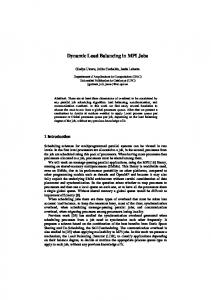
Figure 1 shows a representation of the polymer model. Spring interactions are shown as thin solid lines and Van der Waal interactions with arrowed dashed lines. We can see the two levels of decomposition here. The spatial decomposition is carried out by assigning di�erent beads to di�erent processors. In this example we might assign beads 1, 2, 3 and 4 to the rst processor, and beads 5, 6, 7 and 8 to a second processor. The second level of decomposition, at the interaction level, is carried out by decomposing the Van der Waal interactions. The harmonic interactions (springs between beads) are nearly balanced between the processors already, since every bead has two harmonic interactions, except for the rst and last bead (in this example, with the spatial decomposition carried out on just two processors the workload due to harmonic interactions is exactly balanced). If we count up the Van der Waal interactions as in table 1, we see that processor 1 would have 14 work units to calculate, while processor 2 would be assigned 8. This level of imbalance (where one processor would take approximately twice as long to complete its calculations as others is common in this model). Assigned to Processor 2
Assigned to Processor 1 3
8 7
2 4
1
6
5
Figure 1: Example polymer con guration showing the two levels of possible decomposition. Spatial decomposition is shown using dotted boxes around the rst 4 and the second 4 beads. Harmonic interactions are shown as thin solid lines, Van der Waal interactions as thick arrowed dashed lines. Work unit decomposition takes place at the Van der Waal interaction level. 1 2 3 4 5 6 7 8 Bead Number Num. Harmonic Interactions 1 2 2 2 2 2 2 1 Num. Van der Waal Interactions 3 3 3 5 2 3 2 1 Table 1: Number of interactions (harmonic and Van der Waal) for example polymer con guration shown in gure 1 The two description levels of the problem are modeled using a single graph-theoretic formulation, which acts as the basis for the algorithm formulation in the next section. The problem is represented as a set of nodes V = f(vi ; ni)g; ni 2 , and edges between these nodes. Each node vi has a corresponding weight ni which represents the amount of work contained within that node. To represent topological problems two edge sets are IN
3
used. Edges represent calculations due to a pair of work nodes interacting. The rst set E s is the set of xed static edges. Since these edges are xed in time an initial static decomposition may be used. The second set consists of the dynamic edges, which depend on time, Etd . Spatial decomposition is based on a mapping of the work nodes (V ) to processing nodes, while the second level is obtained from a mapping of the dynamic edge set to the processing nodes. In the algorithm description the edges in Etd are represented by work units wji contained within the work nodes. These work units are much closer in size (amount of processing work) to each other than the nodes are, i.e. the work units are more homogeneous than the work nodes. A good mapping from application to processors will take into account both the load balance and the minimization of communication. For our purposes we assume we have an initial mapping � of work nodes V to the set of processing nodes P = fpig. To preserve the decomposition locality all the work units are assigned an order according to the topology. Let Ni be the total number of work units assigned to the processing node pi, X nk : Ni = k
� (vk )=i
Then the work unit index of wji , the j th work unit within the processing node vi is given by X Iji = j + Ni : (1) k