previously been shown to recreate complex turbulent phenomena (Sharma & McKeon ... Figure 1. Resolvent framework, which maps the nonlinear forcing, fk, at a ..... Inoue, M., Mathis, R., Marusic, I. & Pullin, D. I. 2012 Inner-layer intensities.
Center for Turbulence Research Proceedings of the Summer Program 2016
305
Toward low order models of wall turbulence using resolvent analysis By K. Rosenberg†, T. Saxton-Fox‡, A. Lozano-Dur´an, A. Towne A N D B. J. McKeon†
Resolvent analysis for wall turbulence has the potential to provide a physical basis for both sub-grid scale and dynamic wall models for large-eddy simulations (LES), and an explicit representation of the interface between resolved and modeled scales. Toward the development of such a wall model, direct numerical simulation results are used to represent the Reynolds stresses, formulated as the nonlinear feedback (forcing) to the linear(ized) Navier-Stokes equations. It is found from direct calculation of the Reynolds stress gradients that the (solenoidal) nonlinear feedback is coherent and consistent with energetic activity that is localized in the wall-normal direction. Further, there exists a spatial organization of this forcing that is correlated with individual (large) scales. A brief outlook for LES modeling is given.
1. Introduction McKeon & Sharma (2010) proposed a resolvent framework for wall-bounded turbulent flows, reformulating the Navier-Stokes equations into an input-output system between the nonlinear term and the turbulent velocity and pressure fields. The linear dynamics are considered as a transfer function that maps the nonlinear term, explicitly the spatial gradients of the Reynolds stress tensor (treated as a forcing), to a velocity response. By Fourier-decomposing in the statistically homogeneous directions and performing a singular value decomposition, McKeon & Sharma (2010) identified the first singular vectors at each wavenumber (streamwise, spanwise, and temporal) as highly amplified resolvent response modes. These response modes form an efficient wall-normal basis to model the turbulent velocity field; the superposition of only a few resolvent response modes has previously been shown to recreate complex turbulent phenomena (Sharma & McKeon 2013; McKeon et al. 2013). In this work, preliminary steps were taken to exploit information encoded in both the (linear) resolvent and the nonlinear forcing to inform LES models and form the basis for a low-order representation of wall turbulence. The forcing was calculated directly from direct numerical simulation (DNS) of a turbulent channel flow and the spectral characteristics explored. Then the spatial phase relationships between large scales, which would be resolved by an LES, and small scales, which potentially would not, were characterized using the turbulent boundary layer DNS of Wu et al. (2014). A schematic of the Navier-Stokes equations expressed in terms of the resolvent is shown in Figure 1. At every triplet of streamwise and spanwise wavenumbers and temporal frequency, k = (kx , kz , ω), the resolvent Hk = H(kx , kz , ω) is the transfer function between † Graduate Aerospace Laboratories, California Institute of Technology ‡ Mechanical and Civil Engineering Department, California Institute of Technology
306
Rosenberg et al.
H (κ x , κ z , ω)
Figure 1. Resolvent framework, which maps the nonlinear forcing, ˆfk , at a given streamwise and spanwise wavenumber and temporal frequency, k = (kx , kz , ω), into a velocity, ˆ k , (and pressure) response. Adapted from Moarref et al. (2013). FT and IFT denote u the forward and inverse Fourier transforms, respectively. nonlinear forcing and velocity response (shown for a divergence-free basis), ˆ k (y) = Hkˆfk (y), u
(1.1)
ˆ fu ˆfk = fˆv = − < u ˆ · ∇ˆ u >k , ˆ fw
(1.2)
where
i.e., fk arises from the interactions between pairs of scales (cleanly defined in Fourier space) whose wavenumbers and frequencies sum to k and u denotes the fluctuating component of the Reynolds-decomposed velocity field. In this way, triadically consistent interactions arise naturally in the resolvent framework. Resolvent response modes represent the fluctuations most amplified by solely linear mechanisms; it is not obvious a priori that linear dynamics should be sufficient to describe the system characteristics. While the nonlinear forcing is necessary to close the dynamical system, earlier work has shown that the active part of the forcing can be small in magnitude (because the amplification can be very large, e.g., McKeon & Sharma 2010) and that its magnitude can be crudely approximated as constant over a wide range of k without sacrificing fidelity of the representation of the velocity field (Moarref et al. 2013) because of the selective amplification of the resolvent operator. More attention to the relative phases of response modes, however, is required in order to obtain a self-sustaining model system that can be used in LES modeling. Perhaps surprisingly, the characteristics of the Reynolds stresses in wall turbulence have not been fully explored in the format expressed in Eq. (1.2). However, there are
Toward low-order models of wall turbulence
307
experimental and numerical results from which key pieces of information about the forcing can be obtained. The so-called amplitude modulation coefficient (Mathis et al. 2009) relates large-scale velocity structure to the variation with wall-normal height of the envelope of the small-scale activity. These findings have previously been used to create a predictive model for small-scale velocity statistics based on the large-scale streamwise velocity signal in the logarithmic region (Marusic et al. 2010) that has been applied to LES to improve near-wall small-scale fluctuation statistics (Inoue et al. 2012). The amplitude modulation coefficient can be shown to be dominated by a single large scale (Jacobi & McKeon 2013), and thus gives information on the spatial variation of one term contributing to fˆu (other work shows that other stresses experience the same modulation), which can be exploited in the resolvent framework.
2. Approach We seek interface conditions between small and large scales as required for LES models which exploit the mathematical structure uncovered by resolvent analysis. This question has been addressed by two approaches to modeling the nonlinear forcing using DNS of wall-bounded turbulent flows. First, DNS data of a turbulent channel were used to directly compute the nonlinear or forcing term. The spectral signature of the forcing was interrogated to determine its structure. Second, DNS data of a turbulent boundary layer were used to examine scale interaction and phase relationships as they appear instantaneously. A low-order resolvent model was compared to the instantaneous DNS data and was observed to capture physically realistic scale interaction phenomena.
3. Direct computation of nonlinear forcing In order to compute the nonlinear forcing directly from a fully resolved turbulent flow field, the incompressible Navier-Stokes equations in the form of evolution equations for the normal velocity v and normal vorticity η were solved for turbulent channel flow in a ´ domain of size 12π × 4π using the code described in del Alamo & Jim´enez (2003) ∂∇2 v 1 ∇4 v = hv + ∂t Reτ 1 ∂η ∇2 η. = hη + ∂t Reτ
(3.1) (3.2)
Here the friction p Reynolds number Reτ = huτ /ν = 180, where h is the channel halfheight, uτ = τw /ρ is the friction velocity given by the square root of the mean wall shear stress divided by the density and ν is the kinematic viscosity. The nonlinear terms, hv and hη , from which ˆfk can be determined after a temporal Fourier transform, are given by � � � 2 � ∂ ∂fu† ∂ ∂2 ∂f † hv = − fv† , (3.3) + + w + ∂y ∂x ∂z ∂x2 ∂z 2 ∂f † ∂f † hη = u − w ∂x † ∂z fu fv† = −U · ∇U, fw†
(3.4) (3.5)
308
Rosenberg et al.
where U denotes the full velocity field. As a result, these terms include interactions with the mean velocity and are removed a posteriori to be consistent with the definition of ˆfk given in Eqs. (1.1)-(1.2). Equations (2.1)-(2.2) were advanced with a constant time step to allow for a Fourier transform into the temporal frequency domain, which is desired as the resolvent operator is defined for a particular wavenumber/frequency combination. The time interval at which snapshots were saved and total simulation time were chosen to resolve the frequency content of the flow based on energetic arguments outlined in McKeon et al. (2013), and had respective values of ∆t+ ≈ 3 and tuhτ ≈ 60. The nonlinear terms hv and hη were saved at each time step across the full height of the channel, and for a subset of horizontal wavenumbers (kx , kz ) due to memory restrictions. For simplicity, we limit our attention here to the wall-normal height corresponding to the near-wall cycle, although additional wall-normal information has been analyzed. The structure of the nonlinear forcing was investigated by computing the full threedimensional (kx , kz , ω) spectrum of the various components. Towne et al. (2015) computed and analyzed these forcing terms for a turbulent jet, but to the authors’ knowledge this direct analysis of the spectral content of the nonlinear term for turbulent channel flow using DNS is novel. Previous investigation in the frequency domain has been limited because of the efficiency typically afforded by adjusting the time step. A previous study (Rosenberg & McKeon 2016) used optimization procedures to indirectly ascertain the forcing spectrum giving rise to the velocity and pressure fields at a similar Reynolds number; this approach was limited to the use of time-averaged DNS data and thus lacked the explicit frequency content available in the present study. Various two-dimensional views of the solenoidal forcing spectrum, i.e., integrated over one variable in the (kx , kz , ω) triplet, are discussed here to illustrate the active spatiotemporal scales driving the velocity response. Pre-multiplied spectra of fˆu , fˆv , and fˆw are shown in Figure 2 as a function of streamwise and spanwise wavelengths. Each forcing component appears to be concentrated at relatively small spatial scales, with well-defined + peaks in each case in the vicinity of λ+ x = λz ∼ 100. The wall-parallel components ˆ dominate, with the streamwise forcing, fu , having the largest amplitude. Also shown in Figure 2(d) is the equivalently pre-multiplied leading singular value of the resolvent operator as a function of streamwise and spanwise wavelengths for a fixed wavespeed corresponding to the local mean velocity for y + ≈ 15. The final velocity response is proportional to the product of the singular values and the projection of the forcing onto the singular modes. These plots may provide insight into how the linear response is shaped, and for instance explain the suppression of highly amplified (high singular value) large-scale modes due to a lack of forcing to sustain them. Pre-multiplied spatio temporal spectra as a function of streamwise wavenumber and frequency (Figure 3) also display discernible peaks, with most activity occurring at relatively high frequencies. The concentration of the forcing around a diagonal line reflects a mostly constant convection velocity, c = ω/kx , implying that the stress gradients arising from the triadic interactions sustaining the turbulence in this region of the flow are all localized in the wall-normal direction. The Reynolds stress gradients that lead to a large velocity response via Eq. (1.1) are constrained to be associated with a stress envelope that travels at a convection velocity equal to that of the velocity response by triadic consistency; however, Figure 3 indicates that the gradients determined from DNS are also predominantly associated with the same convection velocity, again stressing local interactions.
Toward low-order models of wall turbulence
309
Figure 2. Pre-multiplied spectrum of the forcing as a function of streamwise and spanwise wavelengths for (a) fˆu , (b) fˆv , and (c) fˆw at y + ≈ 15. (d) The (equivalently premultiplied) leading singular value as a function of streamwise and spanwise wavelengths ¯ (y + ≈ 15) ≈ 10. Note: colorbar in (d) is scaled logarithmically. for c+ = U Overall, Figures 2 and 3 imply coherence to the nonlinear forcing, in contrast to the findings of the forcing that is most amplified in a compressible jet flow obtained using empirical resolvent mode decomposition (Towne et al. 2015). Though not reported here, the forcing showed a similar level of coherence throughout the height of the channel; a more in-depth study of the spectrum to characterize this coherence and its origins is a topic of ongoing work.
4. Scale interaction in instantaneous fields The second approach considered the nonlinear term by studying the interaction of scales in DNS velocity fields. The zero-pressure-gradient turbulent boundary layer DNS data of Wu et al. (2014) at Reθ = 3000, where θ is the momentum thickness, were analyzed to identify the spatial phase relationships between large-scale fast and slow streamwise velocity excursions, small-scale activity and isocontours of instantaneous velocity. We define the (Reynolds-decomposed) fluctuating velocity field, u′ (x, y, z, t), as the difference between the instantaneous velocity u(x, y, z, t) and the streamwise local (spanwise-
310
Rosenberg et al.
Figure 3. Pre-multiplied spectrum of the forcing as function of streamwise wavenumber and frequency for (a) fˆu , (b) fˆv , and (c) fˆw at y + ≈ 15. averaged) mean field U (x, y) to account for streamwise growth of the boundary layer, u′ (x, y, z, t) = u(x, y, z, t) − U (x, y).
(4.1)
Large- and small-scale components of this field were isolated using a low-pass threedimensional Gaussian filter with a standard deviation of σ = 0.1δ, such that the largescale signal, u ˜, is given by R ′ u (X, Y, Z, t)G(x − X, y − Y, z − Z)dXdY dZ R u˜(x, y, z, t) = V , (4.2) G(x − X, y − Y, z − Z)dXdY dZ V
with
1 G(x, y, z) = √ exp σ π and the small scale signal by
�
x2 + y 2 + z 2 σ2
�
,
(4.3)
us = u′ − u ˜. (4.4) The subscript V denotes a volume integral performed over the entire three-dimensional spatial domain. A similar approach was used in Saxton-Fox & McKeon (2016) to analyze particle image velocimetry results from an experimental turbulent boundary layer. Isosurfaces of the unfiltered, fluctuating streamwise velocity field, u′ , from a single snapshot of DNS of Wu et al. (2014) are shown in Figure 4. A single isosurface of the streamwise velocity field u, roughly corresponding to the convection velocity of the large
Toward low-order models of wall turbulence
311
Figure 4. Visualization of the streamwise velocity field of DNS of a turbulent boundary layer (Wu et al. 2014). Red and blue isosurfaces represent the fluctuating velocity field u′ at ±0.04U∞. The gray isosurface represents a single value of the streamwise velocity field, u, here chosen to be 0.85U∞.
scales as estimated from the velocity time series, is shown in white. The instantaneous relationship between scales is masked by the complexity of the full streamwise velocity; however, a clear spatial organization can be seen after application of the filtering process. Figure 5 shows the filtered streamwise velocity field at the same instant. A clear correlation between the large-scale streamwise fluctuation, u ˜, and the black and white isosurfaces of the small-scale fluctuations, us , can be observed. This can be interpreted as evidence of amplitude modulation, in particular in the attenuation and strength of the small scales away from the wall in the presence of positive and negative large-scale structures, respectively. However, the location of strong small-scale activity is also closely correlated with the isosurface of the instantaneous velocity, u˜ + U = 0.85U∞ . Clearly, the wall-normal location of this isosurface is also dictated by u ˜ via the preceding equation. Resolvent analysis (formally for a channel flow) was used to construct a conceptual model for the implied organization of small-scale activity relative to that of the largescales. Seven resolvent response modes were assembled, centered around the turbulence “kernel”, or triad, identified in Sharma & McKeon (2013), which consists of an energetically dominant large scale and a triadically consistent pair of smaller scales, all with the same convection velocity. Four additional small-scale modes possessing different temporal frequencies and therefore different individual convection velocities were incorporated into the present representation. Identifying the largest scale with u˜, the other six modes represent the small-scale activity, us . The phase relationship between the large and small scales was chosen to match the observations of Mathis et al. (2009) and Jacobi & McKeon (2013), namely that the small scales are in phase with the large scale near the wall, out of phase far from the wall, and lead the large scale by π/2 (in space) at the wall-normal location corresponding to the peak amplitude of the large scale. Note that although the set of small scales contains different convection velocities, the streamwise stress can travel at the same convection velocity as the large scale. Figure 6(a) shows the streamwise velocity field associated with the superposition of these seven resolvent modes. Through the beating of the small scales and an appropriate
312
Rosenberg et al.
Figure 5. Visualization of the filtered streamwise velocity field of turbulent boundary layer DNS (Wu et al. 2014) between the spanwise locations z/δ = 0.3 − 0.8. Red and blue contours represent the large-scale fluctuation, u ˜, defined in Eq. 4.2. The white and black isosurfaces represent the small-scale fluctuations, us , at ±0.06U∞, defined as the remainder after filtering the velocity field. The green isosurface represents an isosurface of the large-scale-plus-mean field (˜ u + U ) at 0.85U∞, which is approximately the convection velocity of the large scale, u ˜.
representation of the wall-normal variation of the velocity at different scales, the strength of the small-scale signal is seen to be correlated with, or modulated by, the presence of the large scales. The resolvent model, with phase relationships approximated from experimental statistics, is able to capture many of the structural features associated with the concepts of amplitude modulation and the DNS observations. The localization of regions of small-scale activity around the isocontour of the streamwise velocity field can be observed in both Figure 5 and Figure 6(b), where the green surfaces represent isosurfaces of the large-scale streamwise velocity field (˜ u + U ). The height of the surface tracks the regions of strong small-scale activity in both figures. This correlation is expected to occur for a wide range of energetic large scales in the flow. Thus, importantly for modeling purposes, it is proposed that spatial regions of strong modeled (small) scale activity can be predicted given a range of resolved (large) scale signals. The connection between isosurfaces of the large-scale flow and the localization of small scales is reminiscent of behavior noted in exact coherent states, where small-scale perturbations have been observed to localize about corrugated critical layers (Wang et al. 2007; Hall & Sherwin 2010; Park & Graham 2015) at which the convection velocity is equal to the local mean velocity. While a clean interpretation of a corrugated critical layer in fully turbulent flow is challenging, we have shown that regions of strong small-scale activity are correlated with isosurfaces of the large-scale velocity field, suggesting the potential for analytical and empirical developments concerning representation of small scales given the large-scale field.
Toward low-order models of wall turbulence
313
Figure 6. Superposition of seven resolvent response modes (see Sharma & McKeon (2013) for details on the core modes chosen). (a) The large-scale mode in red and blue at ±25% of the mode’s maximum amplitude. Black and white show isosurfaces of the sum of six small-scale modes at ±5% of the sum’s maximum amplitude. The phases of all modes are set to match observations of Mathis et al. (2009). (b) An isosurface of the large-scale-plus-mean field at 0.6U∞ , which is the convection velocity of the large-scale mode.
5. Summary and conclusion Two approaches to characterizing the nonlinear forcing that appears in the resolvent analysis formulation have been investigated: direct calculation of the solenoidal forcing (Reynolds stress gradients) in a turbulent channel flow and an investigation of the spatial organization of the streamwise stress relative to scales that would be resolved by LES. The goal is to provide for LES wall models physical insight and formal design guidelines that exploit the mathematical structure of the resolvent operator. A low-order model constructed using only seven resolvent response modes has been shown to capture scale interaction phenomena in a physically meaningful way, supporting the potential to use the analysis to provide rules for the interface between modeled and resolved scales in LES. Future work entails projecting the nonlinear forcing obtained directly from the DNS onto singular modes of the resolvent operator to compute low-order representations of the velocity field and to further analyze the interplay between linear and nonlinear mechanisms in wall turbulence and how this regulates self-sustaining processes. There is evidence to suggest that the forcing, as well as the velocity response, can be well modeled by a low-rank approximation (limited numbers of singular functions). Additionally, we seek to compute and better understand the triadic interactions which give rise to the stresses and the nonlinear forcing. Acknowledgments Discussions with other CTR Summer Program participants, especially Mihailo Jovanovic, Peter Schmid, Xiaohua Wu and Armin Zare, were extremely helpful to the development of this work. The authors acknowledge use of computational resources from the Certainty cluster awarded by the National Science Foundation to CTR.
314
Rosenberg et al. REFERENCES
´ del Alamo, J. C., & Jim´ enez, J. 2003 Spectra of the very large anisotropic scales in turbulent channel. Phys. Fluids. 6, L41–L44. Hall, P. & Sherwin, S. 2010 Streamwise vortices in shear flows: harbingers of transition and the skeleton of coherent structures. J. Fluid Mech. 661, 178–205. Inoue, M., Mathis, R., Marusic, I. & Pullin, D. I. 2012 Inner-layer intensities for the flat-plate turbulent boundary layer combining a predictive wall-model with large-eddy simulations. Phys. Fluids. 24, 075102. Jacobi, I. & McKeon, B. J. 2013 Phase relationships between large and small scales in the turbulent boundary layer. Exp. Fluids. 54, 1481. Marusic, I., Mathis, R. & Hutchins, N. 2010 Predictive model for wall-bounded turbulent flow. Science 329, 193–196. Mathis, R., Hutchins, N. & Marusic, I. 2009 Large-scale amplitude modulation of the small-scale structures in turbulent boundary layers. J. Fluid Mech. 628, 311–337. McKeon, B. J. & Sharma, A. S. 2010 A critical-layer framework for turbulent pipe flow. J. Fluid Mech. 658, 336–382. McKeon, B. J., Sharma, A. S. & Jacobi, I. 2013 Experimental manipulation of wall turbulence: A systems approach. Phys. Fluids. 25, 031301. Moarref, R., Sharma, A. S., Tropp, J. A. & McKeon, B. J. 2013 Model-based scaling and prediction of the streamwise energy intensity in high-Reynolds number turbulent channels. J. Fluid Mech. 734, 275-316. Park, J. S. & Graham, M. D. 2015 Exact coherent states and connections to turbulent dynamics in minimal channel flow. J. Fluid Mech. 782, 430–454. Rosenberg, K. & McKeon, B. J. 2016 Data-driven optimization of the forcing in the resolvent analysis of wall turbulence. Proceedings of the International Conference on Theoretical and Applied Mechanics 2016. Saxton-Fox, T. & McKeon, B. J. 2016 Scale interactions and 3D critical layers in wall-bounded turbulent flows. Proceedings of the International Conference on Theoretical and Applied Mechanics 2016. Sharma, A. S. & McKeon, B. J. 2013 On coherent structure in wall turbulence. J. Fluid Mech. 728, 196–238. Towne, A., Colonius, T., Jordan, P., Cavalieri, A. V. & Bres, G. A. 2015 Stochastic and nonlinear forcing of wavepackets in a Mach 0.9 jet. AIAA Paper 2015-2217. Wang, J., Gibson, J. & Waleffe, F. 2007 Lower branch coherent states in shear flows: transition and control. Phys. Rev. Lett. 98, 204501. Wu, X., Moin, P. & Hickey, J.-P. 2014 Boundary layer bypass transition. Phys. Fluids. 26, 091104.