Towards an AC Optimal Power Flow Algorithm ... - Daniel K. Molzahn

1

Towards an AC Optimal Power Flow Algorithm with Robust Feasibility Guarantees Daniel K. Molzahn∗ and Line A. Roald†

Abstract—With growing penetrations of stochastic renewable generation and the need to accurately model the network physics, optimization problems that explicitly consider uncertainty and the AC power flow equations are becoming increasingly important to the operation of electric power systems. This paper describes initial steps towards an AC Optimal Power Flow (AC OPF) algorithm which yields an operating point that is guaranteed to be robust to all realizations of stochastic generation within a specified uncertainty set. Ensuring robust feasibility requires overcoming two challenges: 1) ensuring solvability of the power flow equations for all uncertainty realizations and 2) guaranteeing feasibility of the engineering constraints for all uncertainty realizations. This paper primarily focuses on the latter challenge. Specifically, the robust AC OPF problem is posed as a bi-level program that maximizes (or minimizes) the constraint values over the uncertainty set, where a convex relaxation of the AC power flow constraints is used to ensure conservativeness. The resulting optimization program is solved using an alternating solution algorithm. The algorithm is illustrated via detailed analyses of two small test cases.

I. I NTRODUCTION The optimal power flow (OPF) problem is an important tool for power system operations that minimizes generation cost subject to constraints that model the power flow physics and enforce engineering limits. The need to maintain security despite the forecast uncertainty and short-term fluctuations that are inherent to many renewable energy sources has prompted the development of methods to account for possible adverse effects of uncertainty within the OPF problem. Significant research efforts have focused on uncertainty modeling in the DC OPF problem, where the linearity of the “DC” power flow approximation simplifies the uncertainty modeling and yields an easier optimization problem. However, applications such as distribution grid optimization and transmission grid security assessment call for network models that use the non-linear “AC” power flow equations, which necessitates solution of non-convex AC OPF problems under uncertainty. This paper focuses on robust feasibility in the AC OPF problem, meaning that the chosen operating point must be secure against all uncertainty realizations within a specified uncertainty set. Even deterministic AC OPF problems are non-convex and generally NP-Hard [1], [2]. A wide variety of algorithms have been applied in order to find locally optimal AC OPF solutions [3]. Recent efforts have provided a broad range of “convex relaxation” techniques for AC OPF problems, which replace the AC power flow constraints by a convex outer approximation. See [4] for a comprehensive survey. Convex relaxations yield a lower bound on the optimal objective value ∗ : Argonne National Laboratory, Energy Systems Div., Lemont, IL, USA. † : Los Alamos National Laboratory, Los Alamos, NM, USA. Support from U.S. Dept. of Energy EERE, contract DE-AC02-06CH11357.

for the original non-convex problem, can certify problem infeasibility, and, if certain conditions are satisfied for exactness of the relaxation at its solution point, provide the globally optimal solution to the original non-convex problem. Despite substantial progress in AC OPF solution techniques, the development of rigorous algorithms with probabilistic or robust guarantees for AC OPF problems remains difficult. The non-convexity of the constraints challenges existing methods that provide guarantees for a continuous uncertainty set based on, e.g., samples or decomposition methods. Most existing approaches circumvent the issue of non-convexity by representing the AC power flow equations using either a linearization or a convex relaxation, combined with either a sample-based or analytic chance-constrained representation [5]–[8], a two-stage robust optimization method that exploits conic duality [9], or two-stage stochastic programs based on a sample-average approximation [10] or Benders’ decomposition [11]. Reference [12] uses a sampling approach that provides a posteriori probabilistic guarantees regarding chance-constraint satisfaction for the non-convex AC OPF problem. Recently, [13] proposed an approach to guarantee robust feasibility through an inner approximation; however, the method seems unable to handle nodal power balance constraints on buses without generation or adjustable loads. One of the most comprehensive approaches to date remains [14]. Based on the full non-convex AC power flow equations, the approach in [14] uses scenario generation to build a set of worst-case scenarios, which are found by maximizing infeasibility of the non-convex AC OPF problem subject to uncertainty and contingencies. Our approach separates the problem of enforcing robust feasibility into two aspects: 1) Guarantee solvability of the AC power flow constraints for all realizations within the uncertainty set. 2) Ensure feasibility of the individual engineering constraints for all realizations within the uncertainty set. Although several of the above mentioned approaches provide solutions that perform well, none of them provide rigorous guarantees for the robust feasibility of the underlying, nonconvex AC power flow constraints. Since several of the algorithms, e.g., [14], search for worst-case realizations subject to the AC power flow constraints, there is no guarantee that realizations which lead to AC power flow insolvability will be discovered. Further, none of the above robust approaches truly provide robust feasibility guarantees for the original nonconvex problem. Some rely on the (strong) assumption that their linearization or relaxation provides an exact representation of the AC power flow for all uncertainty realizations or is consistently accurate in identifying the worst-case scenarios. The robust approach in [14] with the full, non-convex AC

2

power flow constraints might run into a local optimum and incorrectly declare robust feasibility while some infeasible scenarios remain. Thus, to the best of our knowledge, no robust AC OPF solution algorithm that is guaranteed to satisfy either aspect has yet been published. We aim to develop an algorithm that addresses this gap. As a first step, the AC OPF algorithm that is the main contribution of this paper focuses on the latter aspect of ensuring engineering constraint satisfaction for all realizations in a specified uncertainty set. This is accomplished by formulating the robust AC OPF problem as a bi-level program where each robust constraint is replaced by a limit on the extreme value achievable within the set of uncertainty realizations. These extreme values are obtained by solving a maximization (or minimization) problem over the uncertainty set, subject to AC power flow constraints. To guarantee conservative estimates of the extreme values, i.e., that the impact of uncertainty is not underestimated, the power flow equations in the constraint maximization problems are replaced by a combination of convex relaxations [15]–[21] (formulated as semidefinite programs (SDP) and second-order cone programs) that balance computational complexity with accuracy. Note that by applying the convex relaxations in this way, we guarantee feasibility of the engineering constraints without any assumptions on the relaxation’s exactness or ability to find worst-case scenarios. To solve the resulting bi-level AC OPF problem, we adapt an alternating algorithm that has been successfully applied to other stochastic AC OPF problems [6], [7]. The algorithm alternates between 1) solving a deterministic, single-level problem with tightened constraint limits and 2) evaluating an optimization problem for each engineering constraint to compute constraint tightenings that ensure feasibility for all uncertainty realizations. The constraint tightenings’ dependence on the operating point (and vice versa) naturally leads to an alternating algorithm. The algorithm has converged to a robustly feasible solution when the tightenings no longer change between iterations. This paper is organized as follows. Section II describes how we model uncertainty and the system’s response to disturbances. Section III formulates the robust AC OPF problem. Section IV details our iterative solution algorithm. Section V provides numerical results. Section VI concludes the paper. II. S YSTEM M ODELING UNDER U NCERTAINTY Based on typical system characteristics, this section presents our models of the power system, the uncertain power injections, and the system’s response to fluctuations. Note that our approach can accommodate a range of variants in addition to our selected modeling choices. A. Notation and System Modeling We consider a power system where N and L denote the sets of buses and lines, with |N | = n. The set of buses with uncertain demand or renewable generation is denoted by U ⊆ N , and the set of conventional generators is represented by G. To simplify notation, we consider one conventional generator, one composite uncertainty source, and one known

injection per bus, such that |G| = |U| = |N | = n. The network √ admittance matrix is denoted Y = G + jB, where j = −1. Each bus i ∈ N has active and reactive power injections pi and qi as well as a voltage phasor with magnitude vi and angle θi . To represent the steady-state behavior of typical power system devices, we use subscripts ( · )P Q , ( · )P V , and ( · )θV to distinguish between PQ buses (specified active and reactive power injections), PV buses (specified active power and voltage magnitude), and a single θV (specified voltage magnitude and angle reference) bus. Each generator i ∈ G has a quadratic cost function with coefficients c2,i , c1,i and c0,i . Each line (`, m)  ∈ L has current  flows into each terminal i`m v ` ˆ `m ˆ `m is the line’s given by = Y , where Y im` vm admittance matrix. We use MATPOWER’s line model [22]. B. Uncertainty Modeling The active and reactive power injections at each bus i ∈ N consist of specified forecasted components, denoted as pinj,i and qinj,i , and fluctuations due to uncertain generation and load demand. Fluctuations in the active power injections, denoted as ω, belong to a specified uncertainty set W. For simplicity, we consider a box uncertainty set,  i.e., each entry of ω lies within a pre-defined interval, ωi ∈ ωimin , ωimax where ωimin ≤ 0 ≤ ωimax . More general uncertainty sets (e.g., budget uncertainty [23]) can also be modeled. Additionally, while this paper does not explicitly consider voltage-dependent loads, extension to more general load models (e.g., ZIP models [24] and induction machine models [25]) is straightforward. We model the fluctuations as having constant power factors cos φi , such that the p reactive power fluctuations are given by (1 − cos2 φi )/ cos φi . Reactive power γi ωi where γi = could also be controlled in a variety of other ways, e.g., as injections that are constant, dispatchable, or participate in voltage control. These types of control can be included in the formulation without any conceptual changes. C. Generation and Voltage Control Setpoints pG0 , qG0 , and vG0 for the active and reactive generation dispatches and voltage magnitudes are scheduled by the system operator based on the forecasted injections, corresponding to ω = 0. During fluctuations ω 6= 0, active power deviations from the scheduled setpoints are determined by an Automatic Generation Control (AGC) scheme [26] that divides the mismatch in total active power generation P Ω = ω i∈U i among the generators according P to a vector of prespecified participation factors α, where i∈G αi = 1. While the deviation Ω due to uncertainty is the main source of power imbalance in the system, there is also an additional power mismatch due to changes in the active power losses. The total change in active power loss, denoted by δp, is also split among the generators according to α such that the active power generation is pG,i (ω) = pG0,i − αi (Ω − δp). The reactive power outputs of generators at PV and reference buses, qG (ω), change to keep their voltage magnitudes constant during fluctuations, whereas generators at PQ buses keep their reactive outputs constant at qG0 . Conversely, the

3

voltage magnitudes vG0 are kept constant by the generators at the reference and PV buses, but vary as functions of the fluctuations at PQ buses, v(ω). III. ROBUST O PTIMIZATION P ROBLEM This section describes the robust AC OPF problem and explains the problem’s challenges. A. Problem Formulation Formalizing the system and uncertainty models described in Section II, the robust AC OPF problem is X
min c2,i p2G0,i + c1,i pG0,i + c0,i (1a)

of constraints. The requirement of robust feasibility in (1) can be condensed into two key challenges: 1) The power flow equations (1e)–(1g) must be guaranteed to have a solution for all uncertainty realizations ω ∈ W. 2) No uncertainty realization ω ∈ W may result in violations of the engineering constraints (1h)–(1k). The remainder of this paper focuses on an algorithm for addressing the latter challenge of preventing engineering constraint violations, with the task of rigorously addressing the former challenge left as a subject for future work. To set up the development of our algorithm for ensuring engineering constraint satisfaction, we reformulate (1) as a bi-level program: min

i∈G

subject to (∀i ∈ N , ∀ (`, m) ∈ L, ∀ω ! ∈ W) X pG,i (ω) = pG0,i − αi (ωi ) − δp(ω) ,

(1b)

∀j ∈ {NP V , NθV } , (1c) ∀k ∈ NP Q , (1d) n h  X vk (ω) Gik cos θi (ω) pG,i (ω) + pinj,i + ωi = vi (ω)   k=1 i −θk (ω) + Bik sin θi (ω) − θk (ω) , (1e) n h  X qG,i (ω) + qinj,i + γi ωi = vi (ω) vk (ω) Gik sin θi (ω) k=1   i −θk (ω) − Bik cos θi (ω) − θk (ω) , (1f)

vj (ω) = vG0,j , qk (ω) = qG0,k ,

θθV (ω) = 0,

(1g)

max pmin G,i ≤ pG,i (ω) ≤ pG,i ,

(1h)

max ≤ qG,i (ω) ≤ qG,i , max ≤ vi (ω) ≤ vi , |i`m (ω)| ≤ imax `m , |im` (ω)|

(1i) ≤

imax `m .

c2,i p2G0,i + c1,i pG0,i + c0,i




(2a)

i∈G

i∈U

min qG,i vimin

X

(1j) (1k)

The objective (1a) minimizes the cost of the scheduled active power generation. Constraints (1b)–(1d) model the generators’ responses to fluctuations ω 6= 0 as described in Section II-C. The power flow equations (1e) and (1f) enforce power balance for all uncertainty realizations. Constraint (1g) sets the angle reference. The generation constraints (1h) and (1i) limit the generator power outputs, while (1j) keeps the voltage magnitudes within bounds. The transmission constraints (1k) limit the magnitudes of the current flows on every line. The variables in (1) can be classified into two categories: 1) control variables pG0 , qG0 , and vG0 which represent scheduled setpoints determined by the optimization problem and 2) dependent variables pG (ω), qG (ω), vG (ω), θ(ω), i(ω), and δp(ω) which are implicitly determined by the control model (1b)–(1d) and the power flow equations (1e)–(1g) for all uncertainty realizations ω ∈ W. B. Discussion of Challenges The robust AC OPF problem (1) is a semi-infinite program since the constraints must be satisfied for all realizations within the continuous uncertainty set W. Developing a tractable representation requires reformulating (1) to obtain a finite set

subject to (∀i ∈ N , ∀ (`, m) ∈ L, ∀ω ∈ W) , Constraints (1e)–(1g) for all ω ∈ W,

(2b)

(2c) min {pG,i (ω) s.t. (1b)–(1g), v(ω) ≥ v} ≥ pmin G,i , ˜ max {pG,i (ω) s.t. (1b)–(1g), v(ω) ≥ v} ≤ pmax (2d) G,i , ω∈W ˜ min min {qG,i (ω) s.t. (1b)–(1g), v(ω) ≥ v} ≥ qG,i , (2e) ω∈W ˜ max max {qG,i (ω) s.t. (1b)–(1g), v(ω) ≥ v} ≤ qG,i , (2f) ω∈W ˜ min {vi (ω) s.t. (1b)–(1g), v(ω) ≥ v} ≥ vimin , (2g) ω∈W ˜ max {vi (ω) s.t. (1b)–(1g), v(ω) ≥ v} ≤ vimax , (2h) ω∈W ˜ max {|i`m (ω)| s.t. (1b)–(1g), v(ω) ≥ v} ≤ imax (2i) `m , ω∈W ˜ max {|im` (ω)| s.t. (1b)–(1g), v(ω) ≥ v} ≤ imax (2j) `m . ω∈W ˜ The first challenge of ensuring power flow feasibility is evident by the presence of constraints (1e)–(1g) in (2b). The second challenge of guaranteeing the satisfaction of the engineering constraints for all uncertainty realizations appears in the subproblems in (2c)–(2j). The formulation requires that each constraint is enforced for the ω that maximizes (or minimizes) the respective constraint value, which guarantees feasibility of each separate constraint for all ω ∈ W. Note that the optimization problems in (2c)–(2j) follow the generation and voltage control model (1b)–(1d) and the power flow constraints (1e)–(1g), and include a lower bound on the voltage magnitude v. The lower bound v is selected ˜ to be significantly below ˜practical operating regimes, e.g., 0.5 per unit (p.u.). This bound precludes the possibility of undesirable “low-voltage” solutions in the absence of other engineering constraints (which are not enforced to avoid circular arguments).1 Imposing this bound is not restrictive in practice since the system model is invalid for very low voltages due to under-voltage protection schemes that would disconnect loads and generators prior to reaching such low voltage magnitudes. ω∈W

1 When feasible, the power flow equations (1e)–(1g) are typically satisfied by one “high-voltage” solution with near-nominal voltage magnitudes and possibly many “low-voltage” solutions. These low-voltage solutions are undesirable since they are generally unstable and typically violate engineering constraints (1h)–(1k). Since we do not enforce (1h)–(1k) in the subproblems (2c)–(2j), imposing a lower bound of v screens out these solutions to ˜ avoid unnecessary conservatism that would result from considering them.

4

IV. A N A LGORITHM E NSURING ROBUST F EASIBILITY OF THE E NGINEERING C ONSTRAINTS The robust AC OPF problem requires that the engineering constraints (1h)–(1k) are satisfied for all possible uncertainty realizations ω ∈ W. This section explains our algorithm for enforcing these constraints in three steps. First, we describe our procedure for evaluating each individual constraint at a given scheduled operating point pG,0 , qG,0 , vG,0 . Next, we use our constraint evaluation procedure to represent the robust AC OPF problem as a deterministic AC OPF problem with tightened constraints. Finally, we present our alternating algorithm that leverages the prior two steps to find an operating point that ensures robust feasibility of the engineering constraints. A. Evaluation of the Robust Feasibility Constraints The optimization problems (2c)–(2j) maximize (or minimize) the constraint value with ω ∈ W as an optimization variable, subject to our uncertainty response model governing the balancing behavior of generators and the AC power flow equations. Since the AC power flow equations are non-convex, the optimization problems may return a locally optimal solution that underestimates the impact of uncertainty. Therefore, we replace the non-convex problems (2c)–(2j) with convex relaxations that are guaranteed to return conservative bounds on the worst-case uncertainty impacts. While any relaxation is acceptable, we specifically use a combination of the sparse SDP relaxation [15]–[17] and the QC relaxation [18] along with a variety of improvements [19]–[21]. This choice of relaxations balances computational complexity with tightness in order to avoid overly conservative solutions (i.e., that the impacts of uncertainty are significantly overestimated due to the use of relaxations that are too loose). The QC relaxation [18] requires specified angle difference min max limits θ`m ≤ θ` (ω)−θm (ω) ≤ θ`m , ∀ (`, m) ∈ L, satisfying ◦ min max ◦ −90 < θ`m ≤ θ`m < 90 . We impose these limits in (2c)– (2j). Thus, our implementation implicitly assumes that no uncertainty realization results in very large angle differences. Similar to the assumed prohibition of unreasonably small voltage magnitudes in Sections III, we choose extreme values max min for θ`m and θ`m , e.g., ±60◦ , in order to avoid eliminating relevant portions of the subproblems’ feasible spaces. We iteratively solve the optimization problems: Step 1–Initialization: Solve relaxations of all optimization problems (2c)–(2j) as well as similar problems for the angle differences ∆θ`,m (ω) = θ` (ω) − θm (ω) in order to obtain initial bounds on pG (ω), qG (ω), v(ω), i(ω), and ∆θ`,m (ω). Step 2–Iterative Tightening: The tighter bounds on pG (ω), qG (ω), v(ω), i(ω), and ∆θ`,m (ω) from the previous iteration facilitate the construction of tighter relaxations. Using these tighter relaxations, we again solve relaxed versions of (2c)–(2j) and the problems associated with the angle differences. Similar to “bound tighening” techniques [19], [20], we repeat step 2 until the relaxations cannot be tightened further.

Note that the bounds on the voltage magnitudes v(ω) and the angle differences ∆θ`,m (ω) resulting from this iterative process are typically substantially tighter than the initially min imposed limits, v and θ`m , θmax . This suggests that that our ˜ v(ω) ≥ v `m min max initial assumptions and θ`m ≤ ∆θ`,m (ω) ≤ θ`m ˜ not restrict are sufficiently mild, and do the feasible spaces of (2c)–(2j). B. Representation as Tightened Constraints After evaluating the robust constraints, we compute the difference between the worst-case values and the values for a given scheduled operating point. For active power, this yields λpmax = max {pG,i (ω) s.t. (1b)–(1g), v(ω) ≥ v} − pG0,i , G,i ω∈W ˜ (3a) λpmin = pG0,i − min {pG,i (ω) s.t. (1b)–(1g), v(ω) ≥ v} G,i ω∈W ˜ (3b) By definition, λpmax and λpmin are non-negative and represent G,i G,i the range within which the corresponding value might vary. max , λ min , λv max , λ min , λi Analogous values λqG,i , and qG,i vi `m i λim` , ∀i ∈ N and ∀ (`, m) ∈ L, are computed for all constraints. The robust constraints (2c)–(2j) are tighter than the corresponding deterministic constraints, i.e., considering robust feasibility shrinks the feasible space. As a consequence, λ ≥ 0, and one can interpret λ as providing constraint tightenings that account for uncertainty. We use this interpretation to reformulate (2) as X
min c2,i p2G0,i + c1,i pG0,i + c0,i (4a) i∈G

subject to (∀i ∈ N , ∀ (`, m) ∈ L) Constraints (1e)–(1g) for ω = 0,

(4b)

pmin ≤ pG0,i ≤ pmax , G,i + λpmin G,i − λpmax G,i G,i

(4c)

min qG,i

(4d)

vimin

min ≤ qG0,i ≤ + λqG,i

+ λvimin ≤ v0,i ≤

|i0,`m | ≤ |i0,m` | ≤

imax `m imax `m

− λi`m , − λim` .

max qG,i

vimax

max , − λqG,i

− λvimax ,

(4e) (4f) (4g)

where pG0 , qG0 , v0,i , i0,`m , and i0,m` denote the generator outputs, voltage magnitudes, and current flows corresponding to the scheduled operating point, rather than being functions of the uncertainty realizations ω. Note that (4) is not equivalent to (2) since the AC power flow constraints (4b) are enforced only for the scheduled operating point, i.e., (4b) only considers ω = 0 rather than ensuring power flow solvability for all ω ∈ W. This reformulation reduces the optimization problem from a semi-infinite program to a problem with a finite set of constraints. Under the assumption that power flow solvability for all uncertainty realizations (i.e., existence of a solution to (4b) for all ω ∈ W) is implied by feasibility of the engineering constraints for all ω ∈ W and satisfaction of the AC power flow equations at the scheduled operating point, a solution to (4) guarantees robust feasibility for the original problem (2). Although we expect this assumption to hold for

5

ˆ0 = 0 Initialize: k = 0 and constraint tightenings λ

k ←k+1

|i4,2 | (p.u.)

Compute constraint tightenings: ˆ k+1 = λ(pk , q k , v k ) λ G0 G0 G0

$3210

0.62

Solve deterministic,
single-level AC OPF: k k pkG0 , qG0 , vG0 = arg min (4) ˆk with specified tightenings λ

Original Limit

0.6

$3200 $3190 $3180

0.58

Tightened Limit

$3170 $3160

0.56

$3150

Check convergence: ˆ k+1 − λ ˆ k |) ≤ η ? Is max(|λ

0.54

No

$3140

0.38

Yes Converged to a secure operating point!

0.4

0.42

0.44

0.46

0.48

0.5

|i4,1 | (p.u.) (a) Feasible space for the deterministic AC OPF problem.

Fig. 1. Alternating algorithm for robust AC OPF problems.

C. Algorithm Description Fig. 1 summarizes our algorithm for solving (4). This algorithm (which is similar to an algorithm previously applied to chance-constrained AC OPF in [6], [7]) alternates between 1) solving a deterministic, single-level AC OPF problem based ˆk on a given set of
constraint tightenings, λ , to obtain a solution k k , vG0 at iteration k, and 2) computing the constraint pkG0 , qG0 ˆ k+1 for this solution by evaluating (3) for each tightenings λ ˆ 0 = 0, such constraint. The algorithm is initialized with λ that the first iteration solves the deterministic, single-level problem associated with the forecasted values (ω = 0). For the deterministic, single-level AC OPF problems (4) solved in each iteration, any solution algorithm can be applied. The algorithm converges when the changes in the constraint tightenings between subsequent iterations are within a specified ˆ k+1 ˆ k threshold η > 0, i.e., λ − λ ≤ η. While this algorithm may fail to converge or yield a suboptimal solution, it has been observed to perform well for other AC OPF problems under uncertainty, such as chanceconstrained AC OPF [6], [7], and the empirical results discussed in the following section are promising. V. N UMERICAL R ESULTS A. Implementation The algorithm is implemented using MATPOWER [22] to solve the deterministic AC OPF problem in each iteration. The

0.62

|i4,2 | (p.u.)

many practical systems, providing more rigorous guarantees regarding power flow solvability is an important aspect of our ongoing work. Reformulating problem (2) as (4) does not directly indicate a viable solution algorithm since the tightenings λ do not have explicit representations. However, as described above, computing appropriate tightenings λ for a given scheduled operating point pG0 , qG0 , vG0 is tractable. Moreover, the optimization problem (4) is a tractable deterministic, singlelevel problem if the values of the tightenings λ are specified. We next present an algorithm that exploits these observations to ensure robust feasibility of the engineering constraints.

Original Limit

0.6 0.58

Tightened Limit

0.56 0.54 0.38

0.4

0.42

0.44

0.46

0.48

0.5

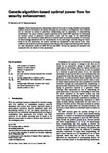
|i4,1 | (p.u.) (b) Uncertainty realizations. Fig. 2. Projections of the feasible space and uncertainty realizations for case6ww.

computation of the tightenings using the relaxations in [15]– [21] is implemented in Matlab and YALMIP [27] with Mosek as a solver. We choose equal participation factors αi = 1/ |G|, ∀i ∈ G. In our experiments, the algorithm typically converges in two to five iterations. For small systems, such as the 6bus system “case6ww” and the IEEE 14-bus system [22], a solution is obtained within two minutes on a laptop with a quad-core 2.70 GHz processor and 16 GB of RAM. Larger systems, such as the IEEE 30-bus or EPRI 39-bus systems, had solution times on the order of 10 to 20 minutes. Rather than being inherent to the algorithm, these solution times are a rough indication of complexity. There are several ways of significantly improving computational speed, particularly by reducing the time required to compute the constraint tightenings. Improving computational speed is an important topic for future work. B. 6-Bus Illustrative Example Fig. 2 illustrates algorithmic performance using the 6-bus system “case6ww” from [22]. The uncertainty set considered for this example is ±5% variation around the forecasted value at every load bus. The algorithm converges in three iterations. 1) Impact of Robustness on AC OPF Solution: The colored region in Fig. 2a is a projection of the feasible space for the

6

Alternating Algorithm PG (MW) QG (MVAr) 97.24 19.21 56.16 71.03 64.05 88.45

“case6ww” system computed using the approach in [28]. The region surrounded by the blue dashed curve corresponds to the feasible space of the deterministic AC OPF problem solved in the final iteration of the alternating algorithm. The solid black line indicates the original deterministic limit on the line flow i4,2 while the dashed black line indicates the tightened flow limit. The red square and blue star correspond to the solution of the original deterministic AC OPF problem and the robust solution based on the alternating algorithm, respectively. The robust algorithm introduces non-zero constraint tightenings λ to account for the impact of uncertainty, hence reducing the feasible space of the deterministic problem (4) that optimizes the operating point for ω = 0. This results in 1.2% higher operating cost for the robust operating point (blue star) relative to the solution without considering uncertainty (red square). Table I compares the generator outputs for the solution to the original deterministic AC OPF problem and the result of the alternating algorithm. Ensuring robustness results in substantially different operation for this test case. 2) Evaluation of Robust Feasibility: Fig. 2b shows the operating points corresponding to 1000 randomly sampled uncertainty realizations based on the solutions from the original deterministic AC OPF problem (red) and the robust algorithm (blue). While many of the red dots indicate violations of the operational limit on i4,2 (i.e., they are above the current limit indicated by the black line), all uncertainty realizations associated with the output of the alternating algorithm result in feasible operation (remain below the black line). This result shows the robustness of the solution from our algorithm. The yellow triangles in Fig. 2b correspond to points where the SDP relaxation used in the last iteration of the alternating algorithm is exact and therefore yields a physically meaningful extreme uncertainty realization. In particular, the SDP relaxations associated with maximizing current flow magnitudes are exact. As a result, the corresponding yellow triangles are at the extrema of the uncertainty realizations denoted by the blue dots. If the relaxations for these constraints had not been exact, the strict bounds resulting from the relaxations would yield tighter constraints and thus a more conservative operating point (i.e., the feasible space enclosed by the blue dashed line in Fig. 2a would shrink, and the largest uncertainty realizations in Fig. 2b would shift down, away from the limit). C. IEEE 14-Bus System We next present results for the IEEE 14-bus system [29] with ±1 to ±30% variation relative to the forecast for every load. We reduce the line flow limits to 25% of the nominal values specified in [29] to obtain interesting behavior. 1) The Impact of Uncertainty on Cost: Fig. 3 shows the cost of the robust AC OPF solution for varying levels of

1.06 1.04 1.02 1 0

5 10 15 20 25 Uncertainty level [% of load]

30

Fig. 3. Cost of the robust AC OPF solution for the IEEE 14-bus system with varying levels of uncertainty. The cost is shown relative to the deterministic solution. Reactive Power

15

Tightening [p.u.]

Deterministic Problem PG (MW) QG (MVAr) 66.46 29.40 76.72 61.26 73.57 85.79

Tightening [MVAr]

Generator 1 2 3

Cost (relative to deterministic OPF)

TABLE I G ENERATOR OUTPUTS FOR CASE 6 WW

λqmin G,6

10

λqmin

5

G,1

Current Magnitude

0.2

λi7,8 λi2,3

0.1

λi1,5 0

0 0

10

20

30

Uncertainty level [% of load]

0

10

20

30

Uncertainty level [% of load]

R-Tightening (based on relaxation) Max. Difference (between R-Tightening and PF-Tightening)

Fig. 4. Tightenings for the binding constraints corresponding to reactive power (left) and current magnitude (right) limits for various levels of uncertainty. The black dashed lines correspond to the R-Tightenings for each active constraint, computed based on the relaxations. The green lines show the maximum differences among the binding constraints between the R-Tightenings and the power flow solutions for the corresponding worst-case scenarios.

uncertainty. We observe that the cost increases for larger uncertainty ranges. This cost increase is due to the larger constraint tightenings λ, which are required to ensure security against larger fluctuations. To avoid unnecessarily high costs, it is important to obtain tightenings that are not overly conservative by using relaxations that are as tight as possible. 2) Conservativeness of Constraint Tightenings: To assess whether the tightenings provide accurate bounds or are overly conservative, we perform an experiment to assess the differences between the bounds obtained from (3) using the power flow relaxations and the bounds we would obtain if we solved the AC power flow equations for the operating point corresponding to the worst-case uncertainty realizations returned by the power flow relaxations (i.e., the decision variables ω returned by the relaxed problems (2c)–(2j)). We denote the former tightenings (used in the iterative algorithm) as the robust tightenings (R-tightenings) and the latter tightenings based on the power flow equations as power flow tightenings (PF-tightenings). The differences between the R-tightenings and the PF-tightenings for the binding constraints provide estimates of the conservativeness introduced by the relaxation. Fig. 4 shows both the values of the R-tightenings and the maximum differences between the R-tightenings and the PF-tightenings for the set of binding constraints. We only show results for constraints on the reactive power injections and current flows because the generator active power constraints are non-binding and the binding voltage constraints correspond to buses where the voltage magnitudes are held constant (PV buses), resulting in tightenings that are equal to zero. The R-tightenings are close to exact for the reactive power

7

injections (differences < 0.1 MVAr), and are also accurate for the current flows (differences ≈ 0.01 p.u.). Although the tightenings increase with increasing uncertainty, the differences between the R-tightenings and the PF-tightenings remain small, indicating that the size of the uncertainty set does not strongly influence the tightness of the relaxations. VI. C ONCLUSION AND F UTURE W ORK This paper proposed the first AC OPF algorithm which provides robust feasibility guarantees for the engineering constraints in the full, non-convex AC OPF problem under uncertainty. To achieve this, we reformulate the problem as a bi-level program where robust feasibility of the individual constraints is enforced by bounding the extreme values that each constrained variable can achieve for any uncertainty realization. We evaluate these extreme values by solving optimization problems based on convex relaxations of the AC power flow equations, which guarantees conservative estimates. We then use the observation that the robust constraints represent a tightening of the deterministic constraints in order to formulate the robust AC OPF as a deterministic problem with tightened constraints, where the tightenings are computed based on the optimization problems. To find a robustly feasible solution that considers the scheduled generation cost, we apply an alternating solution algorithm which first solves the deterministic AC OPF problem with tightened constraints and then updates the tightenings based on the obtained solution. When the algorithm converges, the solution guarantees robust feasibility of the engineering constraints, provided that the power flow equations are feasible for all uncertainty realizations. The effectiveness of the algorithm is illustrated using two small test cases. The results show that ensuring robustness changes both the solution and the associated cost. Further, although the method uses convex relaxations to guarantee conservativeness, the resulting bounds are sufficiently accurate in order to avoid being overly conservative. In future work, we plan to improve computational tractability by identifying and focusing on the most relevant bounds. We also intend to consider more general uncertainty sets and device models. Importantly, we will also extend the method to provide rigorous guarantees on power flow solvability (i.e., the first challenge identified in the introduction) and demonstrate these guarantees using test cases where power flow solvability is crucial to ensuring robustness. R EFERENCES [1] D. Bienstock and A. Verma, “Strong NP-hardness of AC Power Flows Feasibility,” arXiv:1512.07315, Dec. 2015. [2] K. Lehmann, A. Grastien, and P. Van Hentenryck, “AC-Feasibility on Tree Networks is NP-Hard,” IEEE Trans. Power Syst., vol. 31, no. 1, pp. 798–801, Jan. 2016. [3] A. Castillo and R. P. O’Neill, “Survey of Approaches to Solving the ACOPF (OPF Paper 4),” US Federal Energy Regulatory Commission, Tech. Rep., Mar. 2013. [4] D. K. Molzahn and I. A. Hiskens, “A Survey of Relaxations and Approximations of the Power Flow Equations,” invited submission to Found. Trends Electric Energy Syst., 2018. [5] M. Vrakopoulou, M. Katsampani, K. Margellos, J. Lygeros, and G. Andersson, “Probabilistic Security-Constrained AC Optimal Power Flow,” in IEEE Grenoble PowerTech, Grenoble, France, June 2013, pp. 1–6.

[6] L. A. Roald and G. Andersson, “Chance-Constrained AC Optimal Power Flow: Reformulations and Efficient Algorithms,” to appear in IEEE Trans. Power Syst., 2018. [7] L. A. Roald, D. K. Molzahn, and A. F. Tobler, “Power System Optimization with Uncertainty and AC Power Flow: Analysis of an Iterative Algorithm,” in 10th IREP Symp. Bulk Power Syst. Dynamics Control, Espinho, Portugal, Aug. 2017. [8] A. Venzke, L. Halilbasic, U. Markovic, G. Hug, and S. Chatzivasileiadis, “Convex Relaxations of Chance Constrained AC Optimal Power Flow,” to appear in IEEE Trans. Power Syst., 2018. [9] A. Lorca and X. A. Sun, “The Adaptive Robust Multi-Period Alternating Current Optimal Power Flow Problem,” IEEE Trans. Power Syst., vol. 33, no. 2, pp. 1993–2003, Mar. 2018. [10] D. Phan and S. Ghosh, “Two-stage Stochastic Optimization for Optimal Power Flow Under Renewable Generation Uncertainty,” ACM Trans. Model. Comput. Simul., vol. 24, no. 1, pp. 2:1–2:22, Jan. 2014. [11] A. Nasri, S. J. Kazempour, A. J. Conejo, and M. Ghandhari, “NetworkConstrained AC Unit Commitment Under Uncertainty: A Benders’ Decomposition Approach,” IEEE Trans. Power Syst., vol. 31, no. 1, pp. 412–422, Jan. 2016. [12] J. F. Marley, M. Vrakopoulou, and I. A. Hiskens, “Towards the Maximization of Renewable Energy Integration Using a Stochastic AC-QP Optimal Power Flow Algorithm,” in 10th IREP Symp. Bulk Power Syst. Dynamics Control, Espinho, Portugal, Aug. 2017. [13] R. Louca and E. Bitar, “Robust AC Optimal Power Flow,” arXiv:1706.09019, June 2017. [14] F. Capitanescu, S. Fliscounakis, P. Panciatici, and L. Wehenkel, “Cautious Operation Planning Under Uncertainties,” IEEE Trans. Power Syst., vol. 27, no. 4, pp. 1859–1869, Nov. 2012. [15] J. Lavaei and S. H. Low, “Zero Duality Gap in Optimal Power Flow Problem,” IEEE Trans. Power Syst., vol. 27, no. 1, pp. 92–107, 2012. [16] R. A. Jabr, “Exploiting Sparsity in SDP Relaxations of the OPF Problem,” IEEE Trans. Power Syst., vol. 27, no. 2, pp. 1138–1139, May 2012. [17] D. K. Molzahn, J. T. Holzer, B. C. Lesieutre, and C. L. DeMarco, “Implementation of a Large-Scale Optimal Power Flow Solver Based on Semidefinite Programming,” IEEE Trans. Power Syst., vol. 28, no. 4, pp. 3987–3998, Nov. 2013. [18] C. Coffrin, H. L. Hijazi, and P. Van Hentenryck, “The QC Relaxation: A Theoretical and Computational Study on Optimal Power Flow,” IEEE Trans. Power Syst., vol. 31, no. 4, pp. 3008–3018, July 2016. [19] B. Kocuk, S. S. Dey, and X. A. Sun, “Strong SOCP Relaxations of the Optimal Power Flow Problem,” Oper. Res., vol. 64, no. 6, 2016. [20] C. Coffrin, H. L. Hijazi, and P. Van Hentenryck, “Strengthening the SDP Relaxation of AC Power Flows with Convex Envelopes, Bound Tightening, and Valid Inequalities,” IEEE Trans. Power Syst., vol. 32, no. 5, pp. 3549–3558, Sept. 2017. [21] K. Bestuzheva, H. L. Hijazi, and C. Coffrin, “Convex Relaxations for Quadratic On/Off Constraints and Applications to Optimal Transmission Switching,” Preprint: http:// www.optimization-online.org/ DB FILE/ 2016/ 07/ 5565.pdf , 2016. [22] R. D. Zimmerman, C. E. Murillo-S´anchez, and R. J. Thomas, “MATPOWER: Steady-State Operations, Planning, and Analysis Tools for Power Systems Research and Education,” IEEE Trans. Power Syst., vol. 26, no. 1, pp. 12–19, 2011. [23] A. Ben-Tal, L. El Ghaoui, and A. Nemirovski, Robust Optimization, ser. Princeton Series in Applied Mathematics. Princeton Univ. Press, Oct. 2009. [24] D. K. Molzahn, B. C. Lesieutre, and C. L. DeMarco, “Approximate Representation of ZIP Loads in a Semidefinite Relaxation of the OPF Problem,” IEEE Trans. Power Syst., vol. 29, no. 4, pp. 1864–1865, July 2014. [25] D. K. Molzahn, “Incorporating Squirrel-Cage Induction Machine Models in Convex Relaxations of Optimal Power Flow Problems,” IEEE Trans. Power Syst., vol. 32, no. 6, pp. 4972–4974, Nov. 2017. [26] M. Vrakopoulou, K. Margellos, J. Lygeros, and G. Andersson, “Probabilistic Guarantees for the N-1 Security of Systems with Wind Power Generation,” in Probabilistic Methods Applied to Power Systems (PMAPS), Istanbul, Turkey, 2012. [27] J. Lofberg, “YALMIP: A Toolbox for Modeling and Optimization in MATLAB,” in IEEE Int. Symp. Compu. Aided Control Syst. Design (CACSD), Sept. 2004, pp. 284–289. [28] D. K. Molzahn, “Computing the Feasible Spaces of Optimal Power Flow Problems,” IEEE Trans. Power Syst., vol. 32, no. 6, pp. 4752–4763, Nov. 2017. [29] C. Coffrin, D. Gordon, and P. Scott, “NESTA, The NICTA Energy System Test Case Archive,” arXiv:1411.0359, Aug. 2016.