Towards Automatic Derivation of a Product Performance Model from a ...

Towards Automatic Derivation of a Product Performance Model from a UML Software Product Line Model Rasha Tawhid

Dorina Petriu

School of Computer Science Carleton University, Ottawa, Canada [email protected]

Dept. of Systems and Computer Engineering Carleton University, Ottawa, Canada [email protected]

ABSTRACT

1. INTRODUCTION

Software Product Line (SPL) engineering is a software development approach that takes advantage of the commonality and variability between products from a family, and supports the generation of specific products by reusing a set of core family assets. This paper proposes a UML model transformation approach for software product lines to derive a performance model for a specific product. The input to the proposed technique, the “source model”, is a UML model of a SPL with performance annotations, which uses two separate profiles: a “product line” profile from literature for specifying the commonality and variability between products, and the MARTE profile recently standardized by OMG for performance annotations. The source model is generic and therefore its performance annotations must be parameterized. The proposed derivation of a performance model for a concrete product requires two steps: a) the transformation of a SPL model to a UML model with performance annotations for a given product, and b) the transformation of the outcome of the first step into a performance model. This paper focuses on the first step, whereas the second step will use the PUMA transformation approach of annotated UML models to performance models, developed in previous work. The output of the first step, named “target model”, is a UML model with MARTE annotations, where the variability expressed in the SPL model has been analyzed and bound to a specific product, and the generic performance annotations have been bound to concrete values for the product. The proposed technique is illustrated with an e-commerce case study.

Software Product Line (SPL) engineering is a software development approach that takes advantage of the commonality and variability between products from a family. Commonality defines those characteristics that are common to all SPL members, while variability distinguishes the members of a family from each other and needs to be explicitly modeled and separated from the common parts [5]. The main challenge in the context of SPL approach is to model and manage this variability and to support the generation of specific products by reusing a set of core family assets. SPL aims at improving productivity and decrease realization times by gathering the analysis, design and implementation activities of a family of systems. It is based on the reuse of core assets instead of working from scratch [23]. Clements and Northrop define a product line as a set of software intensive systems sharing a common, managed set of features that satisfy specific needs of a particular market or mission, and that are developed from a common set of core assets in a prescribed way [7].

Categories and Subject Descriptors C.4 [Performance of Systems]: modeling techniques, performance attributes. D.2.4 Software/Program Verification: model checking

General Terms Performance, Design.

Keywords Software Product Line, Software Performance Engineering, model transformation, UML, MARTE.

Permission to make digital or hard copies of all or part of this work for personal or classroom use is granted without fee provided that copies are not made or distributed for profit or commercial advantage and that copies bear this notice and the full citation on the first page. To copy otherwise, or republish, to post on servers or to redistribute to lists, requires prior specific permission and/or a fee. WOSP’08, June 23-26, 2008, Princeton, NJ, USA. Copyright 2008 ACM 1-59593-297-X/XX/XXXX…$5.00.

The Unified Modeling Language (UML) is a well-known widespread notation for modeling software systems. Therefore, it would be beneficial to use UML for specifying and modeling a SPL, in order to get all the advantages of UML, including tool support and standardization. However, since UML does not support modeling variability as required for SPL, several UML extension mechanisms to specify product line variability were introduced by different authors [4][6][10][13] [18][19][23]. Each one of these works proposes a set of stereotypes, tagged values and constraints for SPL, but so far there is no standard UML profile for SPL. The evaluation of software and system designs for non-functional properties such as performance, reliability, and security can be enabled by attaching to the UML model suitable additional information specific to the property to be evaluated [20]. Performance properties can be annotated on UML models by using the UMP Profile for Schedulability, Performance and Time (SPT) or its recent replacement, the UML Performance Profile for Modeling and Analysis of Real-Time and Embedded Systems (MARTE) [14]. The SPT and MARTE profiles define stereotypes and tagged values that can be attached to design model elements, particularly in the architecture, behaviour and deployment specifications. An annotated UML model can be transformed into a performance model and analyzed with known analysis techniques and tools [1][21]. Traditionally, performance analysis models were built “by hand” by specialists in the field, who “abstracted” from the software only the properties of interests. However, in the context of model-driven development, a new approach for constructing analysis models is emerging, where software models with performance annotations are automatically

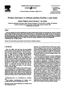
transformed into performance analysis models. A good survey of transformations of software models into different performance models is given in [1]. Examples of such transformations are from UML to Layered Queueing Networks in [16], to Stochastic Petri Nets in [2], and to Stochastic Process Algebra in [3]. In our work we are using the transformation framework PUMA described in [20][21], which converts annotated UML models into different performance models (Layered Queueing Networks, Queueing networks, Petri Nets). This paper proposes a UML model transformation approach for software product lines to derive a performance model for a specific product. The proposed derivation of a performance model for a concrete product requires two steps: a) the transformation of an annotated SPL model to a UML model with performance annotations for a given product, and b) the transformation of the outcome of the first step into a performance model. This paper focuses on the first step as shown in Figure 1, where the input (i.e., the source model), is a UML model of a SPL with performance annotations, which uses two separate profiles: a “product line” (PL) profile similar with [10] for specifying the commonality and variability between products, and the MARTE profile recently standardized by OMG for performance annotations. The source model is generic and therefore its performance annotations must be represented as variables rather than concrete values. The output of this step, the target model, is a UML model with MARTE annotations, where the variability expressed in the SPL model has been analyzed and bound to a specific product, and the generic performance annotations have been bound to concrete values for the product. The proposed technique is

UML -SPL model with UML+MARTE+PL generic performance SPL Model

Feedback

annotations

SPL to Product SPL tomodel Product Model model Transformation Transformation

UML+MARTE UML+MARTE Product Productmodel Model

Performance results and design advice

Performance Solver

UML UML+MARTE model to to Performance model Performance model Transformation (PUMA) Transformation (PUMA)

Performance model Performance model

Focus of the paper

Figure 1. Proposed model transformation approach illustrated with an e-commerce case study, which models the commonality and variability in both structural and behavioural views based on the Product Line UML-based Software Engineering (PLUS) method presented in [10]. Usually, for each individual system, the performance model has to be built from scratch. However, there may be many pre-existing sub-models. This paper aims to take advantage of the SPL engineering approaches by introducing the performance annotations in the early life cycle of the software development process for building the SPL models. Therefore, the derivation of a member of the SPL process not only considers binding the variability expressed in the SPL to a specific product, but also

binding the generic performance annotations to concrete values for this product. The second step of our approach to derive automatically a performance model for a specific product will use the PUMA transformation approach of annotated UML models that has been previously developed in our research group [20] [21]. After the performance model for a product was generated, it can be analyzed with existing solvers and feedback regarding its performance properties will be given to the software development team. PUMA is a tool architecture that provides a unified interface between different kinds of design specifications and different kinds of performance models in the form of an intermediate model called Core Scenario Model (CSM). CSM captures the essence of software performance specification and estimation, and strips away the design detail which is irrelevant to performance analysis. It is suited to the production of performance models of several kinds, as for example layered and regular queuing networks, and stochastic Petri nets [20]. The paper is organized as follows. Section 2 presents the source model for a SPL, and section 3 the target model for a specific product. The model transformation algorithm for deriving the target model is illustrated in section 4. Section 5 discusses related research for managing variability and product derivation in SPL, and Section 6 presents the conclusions and future work.

2. SOURCE MODEL The software product line engineering process consists of two major processes: a) domain engineering for analyzing the commonality and variability between members of the product line and establishing reusable SPL models, and b) application engineering for deriving an individual product that is a SPL member from reusable models defined in the first process rather than starting from scratch. A very important concept in SPL is that of feature, used to represent reusable characteristics of a product line. Features are used to differentiate among members of the product line and to define the commonality and variability in the functionality offered by different SPL products. The feature model is essential for both variability management and product derivation. Gomaa defines in [10] a feature as a requirement or characteristic that is provided by one or more members of the product line. Since UML does not represent features as first-class model elements, the feature model is represented in [10] as a class diagram (see Figure 3, which will be explained in more details later). The stereotypes «common feature», «optional feature», and «alternative feature» are used to distinguish among features that a) must be provided by every members of the SPL, b) need to be provided by only some members, and c) are alternatives to each other, respectively. Related features are grouped into feature groups, which place a constraint on how features are used by a product. Features and feature groups are represented as stereotypes applied to the UML classes that represent features. Different association names are used to model dependencies between features such as requires or mutually_includes and constraints such as mutually_exclusive. In order to model the functional requirements of a SPL, the use case model has to be extended to model the SPL communality and variability. The stereotypes «kernel», «optional», and «alternative» are used to differentiate between use cases that are a) always required by all members of the SPL, b) required

«common feature» E-Commerce Kernel Browse Catalog

Make Purchase Order

«extend»

requires

Process Delivery Order

Confirm Shipment

Create Requisition

Send Invoice

Bill Customer {ext point=Payment}

Confirm Delivery

{mutually exclusive feature}



Pay by CreditC

Pay by Check

«optional feature» Bank mutually includes

«alternative feature» Home Customer requires

Deliver Purchase Order

Mutually includes

«alternative feature» Business Customer

«optional feature» Purchase Order

«at-least-one-of feature group» Payment

«extend»



requires

«exactly-one-of feature group» Customer

«optional feature» Purchase Order

«alternative feature» Home Customer Check Customer Account

«common feature» E-Commerce Kernel

«alternative feature» Business Customer

Prepare Purchase Order

«optional feature» CreditCard Payment

Figure 2. SPL Features represented as use case packages

«optional feature» Check Payment

Figure 3. Feature dependency in the e-commerce SPL

Browse Catalog





Pay by CreditC

Process Delivery Order





Pay by Check

Make Purchase Order



Confirm Shipment



Customer

Check Customer Account

Bill Customer {ext point=Payment}

Create Requisition

Supplier

Send Invoice

Confirm Delivery

Deliver Purchase Order Prepare Purchase Order

Authorization Center Bank

Wholesaler

Figure 4. Use case model of e-commerce SPL

by some but not all members, and c) use cases in which a choice must be made, respectively. Furthermore, the use case variability can be handled through variation points. A variation point is a location in a use case where variation will occur. For small variations, a variation point is identified within the use case scenario to specify a location where the change can take place. However, for complex variations, the “extend” and “include” relationships between use cases may be used to model variations. When modeling the structure of a SPL, variability is introduced

through abstract classes and subclasses and through parameterization. The classes are categorized into “kernel class”, “optional class”, and “variant class” and depicted with stereotypes (see Figure 5). In the behaviour modeling, a sequence diagram or communication diagram is created for each scenario in each use case and categorized as «kernel», «optional», or «alternative», according to the respecting use case. It is also possible to model variability in SPL by using inherited statecharts and parameterized statecharts [10].

In this paper, the source model for the proposed transformation consists of the SPL model with generic performance annotations. We need to make sure that the SPL source model contains all the views necessary for the derivation of performance models: a) structural description of the software showing the high-level software components, especially if they are distributed and/or concurrent; b) the deployment of software to hardware devices, and c) a set of key performance scenarios defining the main system functions frequently executed. The steps for building the source model by a human user are as follows: 12-

345-

6-

Represent the functional requirements as use cases for the SPL. Represent SPL variability through feature modeling. FOR each feature IF the feature is large THEN Represent it as use case package ELSE Represent it as a variation point within a use case IF the variation is small THEN Represent it through a variation point in the use case from step 1 ELSE // The variation is complex Represent it with the extend and include relationships between use cases ENDIF ENDIF ENDFOR Model dependencies and constraints between features through a feature dependency diagram. Represent the structural view as a class diagram for SPL. Model scenarios as sequence diagrams. FOR each use case FOR each scenario Create a sequence diagram annotated with generic performance parameters ENDFOR ENDFOR Model the deployment that ensures maximum distribution.

To illustrate the proposed overall derivation process, we use an ecommerce case study similar to [10] but with some modifications. The e-commerce SPL is a World Wide Web-based product line that handles business-to-business (B2B) as well as business-toconsumer (B2C) systems. For example in B2C, a customer can browse through several catalogs provided by the suppliers to select items to purchase. The customer requests to purchase items from the supplier and provides personal details, such as address and credit card information which are stored in a customer account. If the credit card is valid, a delivery order is created and sent to the supplier. When the order is shipped, the customer is notified and requested to pay. If the system supports several type of payment, the customer has to choose one of them. Optionally, a supplier may create a purchase order requesting new inventory supplies from the wholesaler. The first step for creating our source model, a use case diagram for the e-commerce SPL is built as shown in Figure 4. The kernel use cases (drawn in white) are common to all the e-commerce systems. The light grey use cases are optional and can be used in

either B2B or B2C systems to purchase an order by the supplier. The dark grey use cases are the alternative use cases which are used by only one of the two systems. The use case “Bill Customer” is extended at an extension point called “Payment” within its scenario by two optional use cases “Pay by CreditC” and “Pay by Check”. The extension points are indicated by a tagged value associated to the stereotype of the base use case. In the second step, the kernel use cases are grouped into a common feature called “E-Commerce Kernel”, and depicted as a use case package as shown in Figure 2. The use cases that are used only by the B2C system are grouped into the alternative feature “Home Customer” and the use cases that are used only by the B2B system are grouped into the alternative feature “Business Customer”. The two alternative features “Business Customer” and “Home Customer” are mutually exclusive feature and hence they are grouped into an exactly-one-of feature group called Customer as depicted in the feature dependencies shown in Figure 3. The optional feature “Purchase Order” is realized by the two optional use cases “Prepare Purchase Order” and “Delivery Purchase Order” and hence it is depicted as a use case package. The two optional features “CreditCard Payment” and “Check Payment” are small features and hence they are depicted through an “extend” relationship between use cases. Therefore, both the base use case “Bill Customer” and the extension use cases “Pay by CreditC” and “Pay by Check” have to be selected in order to realize these two optional features. These two optional features “CreditCard Payment” and “Check Payment” are grouped into an at-least-one-of feature group called Payment as depicted in Figure 3. Thus, an individual system can provide one of the features or both of them. Figure 3 depicts dependencies and constraints between features for the third step. In the fourth step, the user creates the class diagram for the ecommerce SPL as shown in Figure 5. The object CustomerInterface behaves differently in B2B systems than in B2C systems. Therefore, a generalization/specialization hierarchy is used to model the different behaviours of this class. The two subclasses B2BInterface and B2CInterface are used by B2B systems and B2C systems respectively. The same happens with the superclass SupplierInterface, which is specialized into two variants POSupplier and Supplier. In the SPL class diagram, each variant or optional class is annotated with the feature that requires it (given through tagged values). In the fifth step, a sequence diagram is created for each scenario in each use case. The case study has 13 scenarios, but only 3 are presented here due to space limitations. The optional sequence diagram “Prepare Purchase Order” is shown in Figure 6, which realizes the optional use case with the same name. The sequence diagram is annotated with generic performance information which has to be bound to concrete values during the derivation of a product. Among these annotations, «PaRunTInstance» is a stereotype indicating which run-time instance of a process executes the lifeline role. It provides an explicit connection between a role in a behavior definition (a lifeline) and a run time instantiation of a process. «GaPerformanceContext» is a performance analysis context with contextParams that are a set of annotation variables defining global properties of this analysis context. Properties of the workload, behaviour, and resources may be defined as functions of such global variables.

Figure 5. Class diagram of e-commerce SPL sd Prepare Purchase Order {contextParams=$ATime} «kernel-vp» «user interface» «PaRunTInstance» {instance = Supplier} :SupplierInterface

«optional» «server» «PaRunTInstance» {instance =PurchaseOrder} :PurchaseOrder

«optional» «server» «PaRunTInstance» {instance =PurchDB} :PurchOrdDB

«kernel» «server» «PaRunTInstance» {instance = Inventory} :Inventory

«optional» «system interface» «PaRunTInstance» {instance =Wholesaler} :Wholesaler

1: PurchaseOrderReq «PaStep» 2: CheckInventory «PaCommStep» «PaStep» {hostDemand=($SupD1,ms), «PaCommStep» msgSize = ($OrderReq,KB)} {hostDemand=($POD1,ms), msgSize = ($Check,,KB)}

3: InventoryLevel «PaCommStep» { msgSize = ($Rep,KB)}

4: StorePurchaseOrder «PaStep» «PaCommStep» {hostDemand=($POD2,ms), msgSize = ($Store,KB)}

6: Confirm «PaCommStep» {msgSize = ($Conf,KB)}

5: PlacePurchaseOrder «PaStep» «PaCommStep» {hostDemand=($POD3,ms), msgSize = ($Place,KB)}

Figure 6. SPL scenario PreparePurchaseOrder

In Figure 6, the first message PurchaseOrderReq is stereotyped as «PaStep» with hostDemand represented by the variable $SupD1, which will be bound to a concrete value when a product is derived. This average processor demand applies to the operation triggered by the message. It applies to the entire operation up until the reply. The message is also stereotyped with the message size (in the «PaCommStep» stereotype).

Figure 7 shows the kernel sequence diagram BrowseCatalog with performance annotations that represent the resource demands made by every scenario step, the scenario workload and the runtime instances in which the life-line roles are running. For instance, the first message GetList has a workload attached with the stereoptype «GaWorkloadEvent» which defines a stream of events driving the system.

sd Browse Catalog {contextParams=$ATime} «kernel-abstract-vp» «user interface» «PaRunTInstance» {instance = CBrowser} :CustomerInterface

«kernel» «server» «PaRunTInstance» {instance = CatServer} :CatalogServer

«kernel » «server» «PaRunTInstance» {instance = CatDB} :CatalogDB

1: GetList «GaWorkload Event» {open(IntArrTime = ($ATime,sec))} «PaStep» «PaCommStep» {hostDemand=($CustD,ms), msgSize = ($GetL,KB), respT={(($ReqT,s,percent95),req), (($CalT,s,percent95),calc)}}

2: GetList «PaStep» «PaCommStep» {hostDemand=($CatSD,ms), msgSize = ($GetL,KB)}

3: ReturnList

4: CatalogInfo

«PaCommStep» {msgSize = ($RetL,KB)}

«PaCommStep» {msgSize = ($RetL,KB)}

Figure 7. SPL scenario BrowseCatalog

sd Bill Customer {contextParams=$ATime} «kernel-vp» «user interface» «PaRunTInstance» {instance = Supplier} :SupplierInterface

«optional» «server» «PaRunTInstance» {instance =Billing} :Billing

1: RequestPayment «PaStep» «PaCommStep» {hostDemand=($SupD1,ms), msgSize = ($OrderReq,KB)}

«kernel» «server» «PaRunTInstance» {instance =DeliOrder} :DeliveryOrder

«optional» «server» «PaRunTInstance» {instance = CAccount} :CustomerAccont

«kernel-abstract-vp» «user interface» «PaRunTInstance» {instance = CBrowser} :CustomerInterface

2: OrderSubscription «PaStep» «PaCommStep» {hostDemand=($BillD1,ms), msgSize = ($OSub,,KB)}

3: OrderNotification «PaCommStep» { msgSize = ($Noti,KB)}

4: AccountRequest «PaStep» «PaCommStep» {hostDemand=($BillD2,ms), msgSize = ($AReq,KB)}

5: Account Info «PaCommStep» {msgSize = ($Info,KB)}

«extension point»{extention=Payment} alt

[CreditCard Payment AND customer chooses CCPayment] ref Pay by CreditC [Check Payment AND customer chooses CheckPayment] ref Pay by Check Pay by Check

Figure 8. SPL scenario BillCustomer

6: RequestPayment «PaStep» «PaCommStep» {hostDemand=($BillD2,ms), msgSize = ($RPay,KB)}

For performance analysis the workload can be open or closed. In our example, the workload is open with an inter-arrival time $ATime (ms). As this variable may appear in several scenarios, it is considered a global annotation variable, and therefore listed as a context parameter in «GaPerformanceContext». The message GetList is also stereotyped with a percentile requirement for the overall response time. Figure 8 shows the sequence diagram “Bill Customer” which realizes the use case with the same name. The extension point “Payment” is depicted as a stereotype on the alt combined fragment. If the alternatives correspond to mutually exclusive features, each product including only one of them, then the sequence diagram for a single product will contain just the right alternative for the given product. If, however, the alternatives correspond to features that are not mutually exclusive (as in this case) each product will contain the alternatives it may chose, and the selection will happen at runtime. Although deployment is not usually represented in SPL models, we need to add a deployment view to the SPL source model. In the sixth step, the user creates the deployment diagram for the SPL assuming maximum distribution. By “maximum distribution” we understand providing the largest number of processors that might ever be used for any product of the SPL, which is not to say that we provide a processor for every artifact manifesting an instance of an active or passive class. For example, if it is known that some instances have to run always on the same processor, this will be reflected in the deployment diagram. The SPL deployment diagram contains all the possible artifacts contained in all the products, even artifacts corresponding to optional or variant classes. Every processing node in the deployment diagram is stereotyped as an execution host. In performance modeling, «GaExecHost» can be any device which executes behavior, including storage and peripheral devices. The node may be stereotyped with communication overheads. The attributes commRcvOverhead and commTxOverhead are the host demand overheads for receiving messages and sending messages, respectively.

3. TARGET MODEL The target model is a UML model with MARTE annotations, where the variability expressed in the SPL model has been analyzed and bound to a specific product. A product model does not contain any more SPL-related stereotypes, tagged values and constraints, because the variability has been resolved. Table 1. Mapping of annotation variables to concrete values Generic parameters

Concrete values

Generic parameters

Concrete values

$SupD1

0.45

$POD2

1.5

$OrderReq

10

$Store

2

$POD3

.0.2 *$Place

$POD1

0.7+.3* $OrderReq

$Check

5

$Place

4

$Rep

10

$Conf

0.5

However, the product model contains performance annotations that have been bound to concrete values, as indicated by the user. The target model for a specific product consists of the following: 1. A use case view for the specific product 2. A product class diagram 3. A product sequence diagram for each scenario in each selected use case 4. A deployment diagram of the product Table 1 shows an example of mapping of the annotation variables from the scenario PreparePurchaseOrder to concrete values, which has to be provided by the user in the form of binding directive to the transformation algorithm presented in the next section. By “concrete values” we don’t mean only literal values, but also expressions in function of annotation variables that may be defined according to MARTE. Another kind of binding that takes place during the derivation of a specific product model from SPL is related to binding the generic roles associated to sequence diagram life-lines to the desired role for handling the chosen feature, as explained in the next section. After obtaining the target model from the source model, it will be transformed to a performance model using the PUMA transformation approach [20][21], as mentioned in Section 1 (see also Figure 1). The target model for our case study is described in the next section, together with the transformation algorithm.

4. MODEL TRANSFORMATION The transformation algorithm supports the automatic derivation of a specific product model from the SPL models. It takes as an input the source model described in section 2 and generates as output the target model for a product presented in section 3. The derivation process starts by selecting the features for the product we want to develop. These chosen features are checked against the feature dependency diagram from the source model to identify any inconsistencies between features. An example is checking to ensure that there no two mutually exclusive features are chosen. The feature model from the source model is used to identify the use cases realizing the chosen features. All the “kernel” use cases have to be included in the product use case diagram, since they represent functionality provided by every members of the SPL. If a chosen feature is realized by a use case package, all the use cases in the package have to be selected. If a chosen feature is realized through “extend” or “include” relationships between use cases, the base use case as well as the inclusion or extension use cases have to be selected. If a feature is realized as a variation point within a use case scenario, this use case has to be chosen as well. Finally, the use case diagram for the product is developed after all the SPL stereotypes were eliminated. The class diagram of the product is created by selecting first all the “kernel” classes from the SPL class diagram. “Optional” and “variant” classes are selected corresponding to the chosen features. In the SPL class diagram, each class is annotated with the feature that requires it. The class diagram of the product is obtained by removing all “optional” and “variant” classes from the SPL model that have not been selected. However, superclasses of the selected “optional” or “variant” classes have to be kept. Other elements to be removed at the end are the stereotypes from the Product Line profile.

For each scenario corresponding to a selected use case, the corresponding sequence diagram is processed next. Each generic role associated to a life-line has to be bound to a specific role according to the selected features (an example on how this is applied will be presented later in the case study). In addition, each generic performance annotation has to be bound to a concrete value, according to the user input. The sequence diagrams for the product are completed after getting rid of the SPL stereotypes. Finally, the SPL deployment diagram has to be tailored to the concrete product. The binding directives indicate the mapping of generic nodes from the SPL diagram to actual nodes for the product (some SPL nodes won’t be necessary for each product, so they will be deleted). The software artifacts for the product are manifestations of the run-time instances indicated by an attribute of stereotype associated to life-line roles in the sequence diagrams derived in step 5 and 6; so the product artifacts are also determined. A high-level description of the transformation algorithm is as follows: Algorithm: ModelTransformation INPUT: SPL source model, selected features and binding directive for the desired product OUTPUT: target model for the desired product BEGIN 1. Select the features that are chosen for the product we want to develop from the SPL feature model. 2. Check the selected features against the feature dependency diagram in the source model to ensure their consistent. 3. Select use cases realizing the chosen features from the SPL use case diagram according to these cases: SWITCH: CASE 1: Feature is realized through use case package THEN Select all use cases in the package; CASE 2: Feature is realized through “extend” or “include” relationships between use cases THEN Select the base use case and the inclusion or extension use cases; CASE 3: Feature is realized through a variation point within a scenario realizing the use case; THEN Select the respective use case; ENDSWITCH 4. Derive the product class diagram from the SPL class dgr. • Select “kernel” classes; • Select “optional” or “variant” classes corresponding to the chosen features; 5. FOR each scenario of the selected use cases Choose the corresponding sequence diagram; ENDFOR 6. FOR each chosen sequence diagram • Bind each generic role associated to a life-line to the desired role for handling the chosen feature; • Bind the performance annotations to concrete values; ENDFOR 7. Build the product deployment diagram from the SPL one • Determine product artifacts from life-line roles; • Bind generic processing nodes to actual ones; • Bind their performance annotations to concrete values END

This algorithm is applied to the e-commerce case study presented din section 2 to derive the business-to-consumer (B2C) model from the e-commerce SPL model. The first step is to choose the features for a specific B2C system. Let us assume that the following features are chosen: alternative feature “Home Customer”, both optional features “CreditCard Payment” and “Check Payment”, and optional feature “Purchase Order”. The common feature “E-Commerce Kernel” has to include, as well. The feature dependency diagram verifies that these features are consistent. The third step selects the four kernel use cases, as well as the two optional use cases “Prepare Purchase Order” and “Delivery Purchase Order” and the alternative use case “Check Customer Account”. Since the B2C system supports both the optional features “CreditCard Payment” and “Check Payment”, the base use case “Bill Customer” and the extension use cases “Pay by CreditC” and “Pay by Check” have to be selected, too. The B2C class diagram is created by selecting first the “kernel” classes from the SPL class diagram. “Optional” classes such as “PurchaseOrder”, “WholeSaler”, and “Bank” have to be selected because they support the optional feature “Purchase Order” as well as the “variant” class “POSupplier”. In addition, the “Optional” classes “Billing”, “CustomerAccount”, “AuthorizationCenter” and the “variant” class “B2CInterface” have to be selected because they support the alternative feature “Home Customer”. Other “optional” and “variant” classes have to be removed. However, the superclasses “CustomerInterface” and “SupplierInterface” are kept. The next step is to select the sequence diagrams that realize the selected use cases. For example, the sequence diagram “Prepare Purchase Order” in Figure 6 is chosen. The generic role “SupplierInterface” has to be bound to the concrete one “POSupplier”, which plays the desired role for handling “Prepare Purchase Order” scenario. The generic performance annotations are bound to concrete values as indicated by the user (an example is shown in Table 1). The sequence diagram “BrowseCatalog” in Figure 7 is also selected, because it realizes the “kernel” use case of the same name. The generic role “CustomerInterface” is bound to the concrete “B2CInterface”, which plays the role that handles the feature “Home Customer”. Finally, the sequence diagram “Browse Catalog” for the B2C system is derived from its SPL counterpart by eliminating the SPL stereotypes and binding the performance annotations. The sequence diagram “BillCustomer” shown in Figure 8 is also selected, as it realizes a selected use case. Since both features “CreditCard Payment” and “Check Payment” are chosen for this product, the alt fragment will contain both alternatives and the choice will happen at run-time. The generic role “SupplierInterface” has to be bound to the concrete one “Supplier”, which plays the desired role for handling “BillCustomer” scenario. Also, the generic role “CustomerInterface” is bound to the concrete object “B2CInterface”. The deployment diagram for the B2C system is depicted in Figure 9. The software components are deployed onto actual processors and the performance annotations are bound to concrete ones.

5. RELATED SPL RESEARCH This section presents existing research related to SPL modeling in UML. SPL requires mechanisms to specify variability and commonalities in UML models, and techniques to manage a set of

constraints and dependencies between features. In addition, approaches to derive products from the SPL are needed. Many authors address variability at structure level, but fewer at behavioural level. In [18] is introduced the UML-F profile that supports product line annotations. The author provides notational elements to specify well known design patterns. This profile is defined for frameworks and is concerned only with structural aspects. A UML extension to support feature diagrams and to describe variability in the UML diagrams is presented in [5]. Stereotypes are used to model “variant” constraints and to show the dependencies between classes. Only UML class diagrams are considered. This work is extended for generic modeling in UML in [6]. Stereotypes for variable features in UML are introduced in [19]. Variability models that can be used during the different life cycle stages of software product lines are presented in [16], describing variability in feature models, use case models, design models, component models, and test models. In [13] it is introduced a UML 2 profile for variability models, which uses activity diagrams to show the impact of variability on the process flow. An approach to extend UML 2.0 to represent variability on the product line architecture is presenetd in [4]. A number of papers from the group led by Jézéquel propose a UML profile for modeling variability at structural and behavioural levels [15][22][23][24][25][26]. In [15], two types of constraints for product line are proposed expressed as OCL constraints at the UML meta-model level. Generic constraints such as inheritance constraint and dependency constraint are applied to any SPL. However, specific constraints such as presence constraint and mutual exclusion constraint are applied to a specific SPL. In [22], a model for behavioural requirements in SPL is introduced. These requirements are expressed by high level message sequence charts extended with constructs for handling variability. An approach for deriving product models from a UML SPL model based on a creational design pattern is proposed in [24]. An UML 2.0 profile for SPL including stereotypes, tagged values, and structural constraints is proposed in [23]. The paper deals with deriving a product model from UML class diagrams and sequence diagrams, by using generic and

specific constraints. In [25], an approach to create detailed behaviour for each product member in the PL is proposed. First, the author uses an algebraic construct to specify variability in the sequence diagrams. Then, the algebraic expressions are interpreted to resolve variability and to derive product expressions which are subsequently transformed to a set of statecharts. An UML model derivation technique for static and behaviour views is proposed in [26]. The static derivation is started from a product line class diagram with a decision model and generates the product class diagram. However, an algebraic approach is proposed to derive statecharts for a specific product from the sequence diagrams of the product line, by transforming product scenarios given as a reference expression for SD into a composition of statecharts. Another group addressing variability at both structural and behavioural levels is Gomaa’s group. An extension to UML for capturing the variability of a product family at the feature and design level is presented in [8]. Variation points are defined implicitly by marking features or classes as optional or variant. Dependencies are modeled by dependency meta-classes and restrict the selection of two variants. In [9] four different approaches to model variability are described, by using parameterization, information hiding, inheritance, and variation points. The paper shows how variation points can be used to model other three different approaches. In [10] is presented a method called Product Line UML-based Software Engineering (PLUS) for modeling explicitly the commonality and variability in a SPL, by extending UML-based modeling methods used for single systems. The product line profile in our proposed technique uses the PLUS method (with some modifications). One of the few papers that proposes tool support for representing multiple view for product lines models stored in a repository is [11]. The paper focuses on the class and feature model. A consistency checking tool is developed to report inconsistencies among the views. Automated support for product derivation from the product line repository at the meta-model level is also proposed in [11]. A modeling approach for dynamic reconfiguration of software architectures is presented in [12]. The software architecture is built out of architectural patterns. For each software architecture pattern, there is a corresponding software reconfiguration pattern, which describes how the architecture can be dynamically adapted.

PurchaseOrderNode

CatalogNode «GAExecHost»

«GAExecHost»

CustomerNode

«artifact»

«GAExecHost»

CatServer

«artifact» CBrowser

BankNode

«GAExecHost»

«artifact» PurchaseOrder

«artifact» Bank

«artifact»

«artifact» PurchDB

CatDB «artifact» WholeSaler

AuthorizationCenter Node

«GAExecHost»

SupplierOrganizationNode «GAExecHost» «artifact» DeliOrder

«artifact» Billing

«artifact» AuthCenter

«artifact» DeliOrdDB

«artifact» CAccount

InventoryNode «GAExecHost»

«artifact»

«artifact»

Supplier

Inventory «artifact» InventoryDB

Figure 9. Deployment diagram of the B2C product

We chose to base our work on Gomaa’s group work, especially on PLUS [10], because it is a well developed method, it is applied to real-time systems and pays a lot of attention to the representation of behaviour, which is very important for performance analysis. Furthermore, PLUS represents the feature model as a class diagram, which is more intuitive than other approaches (for instance, simpler than modeling features as OCL constraints). However, our approach has a few differences from PLUS. Firstly, we use sequence diagrams for modeling behaviour instead of collaboration (communication) diagrams, due to the fact that the modeling power of sequence diagrams has been considerably enhanced in UML 2 with respect to comunication diagrams. Secondly, we pay attention to the deployment of software components to hardware devices, which is also important for performance analysis. Thirdly, we modified the stereotype attributes used in the SPL class diagram to specify the related features.

6. CONCLUSIONS One of the main advantages of the Software Product Lines development process is that it takes advantage of the reusability of a set of core assets shared among the members of a family of products, instead of building each product from scratch. In this paper, we intend to do the same (i.e., reuse performance annotations) when applying Software Performance Engineering techniques in the early phases of the SPL development. Instead of annotating from scratch each UML model of each product, we propose to annotate the SPL model once with generic annotations, and to provide binding information when deriving the annotated model of a desired product from the generic SPL model. This paper proposes a two-step model transformation approach for deriving a performance model for a specific product from an UML model with performance annotations of a SPL. The first step derives automatically a UML model with concrete performance annotations for a specific product from a SPL model with generic performance annotations. The second step transforms the UML+MARTE model obtained in the first step into a performance model by using PUMA, an existing model transformation approach developed in our research group. The paper contributes toward the long-term goal of developing UML-based tool support for early performance analysis of a product from a SPL model. The research challenge here is not only in dealing with generic yet reusable performance annotations, but also with proposing an algorithm that analyses the variability in a SPL model and derives the model of a specific product based on the set of features selected for that product. Although there is a lot of existing research in modeling SPL variability with UML, as surveyed in section 5, we have found only two proposed transformation algorithms for deriving a product from an SPL model [11] and [26]. However, none of these deals with scenarios represented as sequence diagrams, as proposed in our approach. The authors are in the process of implementing the model transformation proposed in this paper on top of the Eclipse framework and connecting it with the PUMA toolset.

ACKNOWLEDGMENT This research was supported by a grant from NSERC, the Natural Sciences and Engineering Research Council of Canada.

REFERENCES [1] S. Balsamo, A. Di Marco, P. Inverardi, M. Simeoni, “Modelbased performance prediction in software development: a survey” IEEE Transactions on Software Engineering, Vol 30, N.5, pp.295-310, May 2004. [2] S. Bernardi, S. Donatelli, and J. Merseguer, “From UML sequence diagrams and statecharts to analysable Petri net models” in Proc. 3rd Int. Workshop on Software and Performance (WOSP02), pp. 35-45, Rome, July 2002. [3] C. Cavenet, S. Gilmore, J. Hillston, L. Kloul, and P. Stevens, “Analysing UML 2.0 activity diagrams in the software performance engineering process” in Proc. 4th Int. Workshop on Software and Performance (WOSP 2004), pp. 74-83, Redwood City, CA, Jan 2004. [4] Y. Choi, G. Shin, Y. Yang, and C. Park, “An approach to extension of UML 2.0 for representing variabilities”, Computer and Information Science, Fourth Annual ACIS International Conference, INSPEC Accession 3, pp.258– 261, 2005. [5] M. Clauss, “Modeling variability with UML”, GCSE 200– Young Researchers Workshop, September 2001. [6] M. Clauss, “Generic Modeling using UML extensions for variability”, In: Workshop on Domain Specific Visual Languages at OOPSLA, Tampa Bay, FL, USA, 2001. [7] P. Clements, and L. Northrop, “Software Product Lines: Practice and Patterns”, p.608, Addison-Wesley, 2001. [8] H. Gomaa, M.E. Shin “Multiple-View Meta-Modeling of Software Product Lines”, 8th International Conference on Engineering of Complex Computer Systems (ICECCS 2002), IEEE Computer Society 2002, pp. 238-246, 2002. [9] H. Gomaa, D. L. Webber, "Modeling Adaptive and Evolvable Software Product Lines Using the Variation Point Model," hicss, p. 90268c, Proceedings of the 37th Annual Hawaii International Conference on System Sciences (HICSS'04) - Track 9, 2004. [10] H. Gomaa, “Designing Software Product Lines with UML: From Use Cases to Pattern-based software Architectures”, Addison-Wesley Object Technology Series, July 2005. [11] H. Gomaa, M. E. Shin “Automated Software Product Line Engineering and Product Derivation”, Proceedings of the 40th Hawaii International Conference on System Sciences, 2007. [12] H. Gomaa, M. Hussein “Model-Based Software Design and Adaptation”, International Conference on Software Engineering Proceedings of the 2007 International Workshop on Software Engineering for Adaptive and Self-Managing Systems Page: 7, 2007. [13] B. Korherr, and B. List, “A UML 2 Profile for Variability Models and their Dependency to Business Processes”, Database and Expert Systems Applications DEXA '07, 18th International Conference, Regensburg, Germany, pp: 829834, Sept., 2007. [14] Object Management Group, UML Profile for Modeling and Analysis of Real-Time and Embedded Systems, OMG Adopted Specification ptc/07-08-04, August 6, 2007.

[15] L. Monestel, T. Ziadi, and J.-M. Jézéquel, “Product line engineering: Product derivation”, In Workshop on Model Driven Architecture and Product Line Engineering, at the SPLC2 conference, San Diego, August 2002.

[21] C.M. Woodside, D.C. Petriu, J. Xu, T. Israr, J.Merseguer, “Methods and Tools for Performance by Unified Model Analysis (PUMA)”, submitted for publication to IEEE Trans. on SE, 2007.

[16] D.C. Petriu, H.Shen, “Applying the UML Performance Profile: Graph Grammar based derivation of LQN models from UML specifications”, in Computer Performance Evaluation (T. Fields, P. Harrison, J. Bradley, U. Harder, Eds.) LNCS 2324, pp.159-177, Springer, 2002.

[22] T. Ziadi, L. Hélouët, and J.-M. Jézéquel, “Modeling behaviors in product lines”, In Proceedings of REPL'02 (workshop on RequirementsEngineering for Product Lines), pages 33–38, Essen, Germany, September 2002.

[17] K. Pohl, G. Böckle, and F. van der Linden, “Software Product Line Engineering: Foundations, Principles, and Technique”, Springer-Verlag Berlin, Heidelberg, 2005.

[23] T. Ziadi, L. Hélouët, and J.-M. Jézéquel, “Towards a UML Profile for Software Product Lines”, In Software ProductFamily Engineering, 5th International Workshop, pages 129– 139, Springer, 2003.

[18] W. Pree, M. Fontoura, and B. Rumpe. “Product line annotations with uml-f”, in Gary J. Chastek, editor, Software Product Lines, Second International Conference, SPLC2, San Diego, CA, USA, August 19-22, 2002, proceedings, LNCS vol 2379, Springer, 2002.

[24] T. Ziadi, J.-M. Jézéquel, and F. Fondement, “Product line derivation with uml”, In Jilles van Gurp and Jan Bosh, editors, Proceedings Software Variability Management Workshop, pages 94–102. University of Groningen Departement of Mathematics and Computing Science, 2003.

[19] S. Robak, B. Franczyk, and K. Politowicz, “Extending the UML for Modeling Variability for System Families” Int. J. Appl. Math. Comput. Sci., Vol.12, No.2, 285–298, 2002.

[25] T. Ziadi, L. Hélouët, and J.-M. Jézéquel, “Behaviors generation from product lines requirements”, In Proc. UML2004 workshop on Software Architecture Description, September 2004.

[20] C.M.Woodside, D.C. Petriu, D.B. Petriu, H.Shen, T.Israr. J. Merseguer, “Performance by Unified Model Analysis (PUMA)”, WOSP’05, Palma de Mallorca, Spain, July 11–15, 2005.

[26] T. Ziadi and J.-M. Jézéquel, “Software Product Lines, chapter Product Line Engineering with the UML: Deriving Products” pages 557-586, Springer 2006.