Towards Axiomatizing the Semantics of UML Activity Diagrams: A ...

Towards Axiomatizing the Semantics of UML Activity Diagrams: A Situation-Calculus Perspective Xing Tan Semantic Technologies Laboratory University of Toronto Email: [email protected]

Abstract—In this paper, the UML activity diagrams are first defined graph-theoretically, with an adoption of the concepts of Petri nets tokens. The semantics of activity diagrams is further axiomatized as a logical action theory called SCAD. Example applications of SCAD are also given. Keywords-UML Activity Diagrams; Situation Calculus Ontology

I. I NTRODUCTION The Unified Modeling Language (UML) activity diagrams are designed for graphical specifications of dynamical aspects of systems. They have been widely used to model work flows of, e.g., business processes and software systems. For each graphical notation of activity diagrams, only a textual description is provided by the Object Management Group (OMG) to define its syntax and semantics [3]. In this paper, we start by providing a graph-theoretic definition for the activity diagrams and formal characterizations of activity diagram dynamics through adopting the concepts of Petri nets tokens. We move on to propose an ontology of activity diagrams called SCAD, standing for SituationCalculus action theory for Activity Diagram; whereas situation calculus (Reiter’s variety, see [2]) is a second-order logic language that provides a rigorous paradigm for axiomatizations of dynamical systems. SCAD contains a set of actions, corresponding to the firing of diagram nodes, and a set of function fluents, corresponding to the number of tokens at diagrams nodes, which are subject to change upon firing actions. The paper also covers two example SCAD applications: one, important mathematical properties of activity diagrams are further axiomatized in SCAD. Consequently, we show that the reachability problem is PSPACE-complete in a subclass of SCAD; two, an example diagram is presented, where the projection problem is investigated in particular. II. UML ACTIVITY D IAGRAMS In this section, graph-theoretic definitions to describe UML activity diagrams are introduced first, and the concept of markings to capture the dynamics of activity diagrams are presented next.

Michael Gruninger Semantic Technologies Laboratory University of Toronto Email: [email protected]

Definition 1: An UML activity diagram is a pair (N, E), where N is a finite set and E is a binary relation on N . The elements in N are called nodes. Each node belongs to one and only one of the following types: Ini, F inal, Branch, M erge, F ork, Join, or Action. The elements in E are called edges. The edge set E consists of ordered pairs of nodes. That is, an edge is a set {u, v}, where u, v ∈ N and u 6= v. By convention, we use the notation (u, v) for an edge, rather than the set notation {u, v}. If (u, v) is an edge in an activity diagram, we say that (u, v) is incident from or leaves node u and is incident to or enters node v. Given a node u ∈ N , the set • u = {v|(v, u) ∈ E} is the pre-set of u, where each v is the input of u, and the set u• = {v|(v, u) ∈ E} is the post-set of u, where each v is the output of u. It is required that 1   = 0 if n is the Ini node = 1 if n is Branch, F ork, Action, or F inal |• u|  = 2 if n is a M erge, or a Join node and   = 0 if n is the F inal node = 1 if n is M erge,Join, Action or Ini |u• |  = 2 if n is a Branch , or a F ork node The concept of tokens and its firing is adopted from Petri nets. In a Petri-net, nodes of places contain tokens whereas firing of a transition node make changes to the number of tokens in the places that enter, or leave the transition node. As defined below, a node in an activity diagram by itself maintains tokens and can fire as long as it contains at least one token. In addition, the left (or right) input of a Join node accepts left (or right) tokens and, intuitively, one left token and one right token will be counted as a full token for the Join node. Definition 2: A marking of a diagram (N, E) is a mapping in the form M K : N → N , to indicate the distribution of tokens on the nodes of the diagram; it can be represented as an vector M K(n1 ), . . . , M K(nm ) where n1 , . . . , nm is 1 In general, the in-degrees of M erge and Join, and the out-degrees of Branch and F ork, all can be integers greater than 2.

an enumeration of the node set N and for all i such that 1 ≤ i ≤ m, M K(ni ) tokens are assigned to node ni . A node n is marked at the marking M K if M K(n) > 0. A marked node u is also enabled and is accepted by every node v ∈ u• . The firing of an enabled node u at M K leads u to the successor marking M K 0 (Written as M K =⇒ M K 0 ). More precisely, 1) if u is a Branch node, then for every node n ∈ N ,  if n = u  M K(n) − 1 {M K(n) + 1, M K(n)} if n accepts u M K 0 (n) =  M K(n) otherwise P and we also have, ni ∈u• M K(ni ) = 1; 2) if u is a non-Branch node, then for every node n ∈ N ,   M K(n) − 1 if n = u M K(n) + 1 if n accepts u M K 0 (n) =  M K(n) otherwise In other words, after the firing of u, a token is removed from u and a token is added to the only node (if u is of type Ini, Action, M erge, Join), each node (if u is of type F ork), one and only one node (if u is of type Branch), in the post-set of u. There is no need to fire a node with type F inal; 3) (Exception of Join) if a token fired by u is accepted by the left (right) in-edge of a Join node n, then M Klef t (n) ( M Kright (n)) is increased by 1. M Klef t (n) = 1 and M Kright (n) = 1 function as one full token at n, i.e., M K(n) = 1. The firing sequence σ = n1 , ..., nm is a sequence of nodes in N . For particular σ and M K, σ is legal at M K if there are marking sequence M K0 , M K1 , ..., M Km such n1 nm that M K = M K0 , M0 =⇒ M K1 , ..., M Km−1 =⇒ M Km σ (written as M K =⇒ M Km ). The reachability problem for an (N, E, M K0 ) is to decide, for some marking M K 0 , if there exists a firing σ sequence σ such that M K0 =⇒ M K 0 . An instance (N, K, M K0 ) is k-bounded if the number of tokens of any node n ∈ N at any M K in the reachability set is bounded by k. III. S ITUATION C ALCULUS The situation calculus is a logical language for representing changes upon actions in a dynamical domain. The language L of situation calculus as stated by [2] is a secondorder many-sorted language with equality. Three disjoint sorts: action, situation, object (for everything else in the specified domain) are included in the language L. For example, rain denotes the act of raining, and putdown(x, y) denotes the act of object x putdown y on the ground. A situation characterizes a sequence of actions in the domain. The constant situation S0 is to denote the empty sequence of actions, whereas the function symbol do is introduced to construct the term do(a, s),

denoting the successor situation after performing action a (such as, in a weather simulation scenario, rain) in situation s. The situation term do(sunshine, do(rain, s)) denotes the situation resulting from first rain and then sunshine, which distinguishes itself from the other situation term do(rain, do(sunshine, s)). It is easy to see that, intuitively, a situation corresponds to a finite sequence of actions. The binary predicate @ specifies the order between situations. For example, s @ s0 stands for that the situation s0 can be reached by performing one or several actions from s. s v s0 is an abbreviation of s @ s0 ∨ s = s0 . In addition, a predicate P oss(a, s) is applied to specify the legality of performing action a in situation s, For example, P oss(rain, s) ⊃ heavyCloudy says that it is possible to rain only if the sky is with heavy cloud. In a particular domain, the language might contain situation independent relations, like matchLocation(T oronto), and situation independent functions, like size(P lot2). However, in many of the more interesting cases, the values of relations and functions change between situations; accordingly, a relational fluent, or a functional fluent, in L is defined as a predicate, or a function, respectively, whose last argument is always a situation (e.g., captain(John, do(catchF ever, S0 )) is a relational fluent, whereas weight(John, do(recover, s)) is a functional fluent). IV. SCAD The ontology of SCAD is formally defined in this section. Aside from situations and actions, objects in SCAD include diagram nodes: Ini, F inal, Action, Branch, M erge, F ork, and Join. Functions of actions in SCAD include • f ireJ(j): firing a Join node; • f ireBl (b): firing a Branch node to its left edge; • f ireBr (b): firing a Branch node to its right edge; • f ire(p): firing a node other than Join and Branch. Functional fluents includes: • T knsJl (j, s): the number of left tokens at a Join node j in situation s; • T knsJr (j, s): the number of right tokens at a Join node j in s; • T kns(p, s): the number of tokens at a non-Join node p in s. Situation-independent relations are defined in SS0 of SCAD, which specifies the structure of an activity diagram and include: • LpreL(m, n): the left output of a (F ork or Branch) node m enters the left input of a M erge or Join node n, LpreR(m, n), RpreL(m, n), and RpreR(m, n) are defined in a similar way; • Lpre(m, n): the left output of a (F ork or Branch) node m enters the only input of node n that is not of type M erge or Join, Rpre(m, n) is defined similarly;

preL(m, n): the only output of a (non-Fork and nonBranch) node m enters the left input of of a type M erge or Join node n, preR(m, n) is defined similarly; • pre(m, n): all cases including the other cases (i.e., the only input of the node m enters the only input of the node n), and all of the above cases; • post(m, n): m leaves n if and only if n enters m. Definition 3: SCAD is defined as a logical theory Sscad , which consists several sets of axioms as follows: •

Sscad = Df ∪ Sap ∪ Sss ∪ Suna ∪ SS0 where • Df is the foundational axioms (see [2] for details); • Sap (action preconditons axioms) – P oss(f ireJ(j), s) ≡ T knsJl (j, s) ≥ 1 ∧ T knsJr (j, s) ≥ 1 (a Join node j is enabled to fire iff the number of left tokens and the number of right tokens of it, both are greater than, or equal to 1); – P oss(f ireBl (b), s) ≡ T kns(b, s) ≥ 1 (a Branch node b is enabled to fire to its left iff the number of tokens it contains is greater than or equals to 1); – P oss(f ireBr (b), s) ≡ T kns(b, s) ≥ 1 (a Branch node b is enabled to fire to its right iff the number of tokens it contains is greater than or equals to 1); – P oss(f ire(p), s) ≡ T kns(p, s) ≥ 1 (a node p is enabled to fire iff the number of tokens it contains is greater than or equals to 1); • Sss (successor state axioms) – T kns(p, do(a, s)) = n ≡ γf (p, t, n, a, s) ∨(T kns(p, s) = n ∧ ¬∃n0 γf (p, t, n0 , a, s)) def where γf (p, t, n, a, s) = γfa (p, n, a, s) ∨ γfb (p, q, n, a, s), referring to the two sets of firing actions that makes the number of tokens at the nonJoin node p on situation do(a, s) to n, that is: def (1). γfa (p, n, a, s) = (n = T kns(p, s) − 1∧ (a = f ire(p) ∨ a = f ireBl (p) ∨ a = f ireBr (p))) (at situation s, the number of tokens at the node p, which is of any type but Join, is (n + 1), and p fires at situation s, making the number of tokens it contains at the subsequent situation do(a, s) decreased by 1); def (2). γfb (p, q, n, a, s) = ((∃q). pre(q, p) ∧ n = T kns(p, s) − 1 ∧ (a = f ire(q)∨ a = f ireBl (q) ∨ a = f ireBr (q) ∨ a = f ireJ(q))) (at situation s, the number of tokens at place p, which is of any type but Join, is (n − 1), and the node q, which is of any type and enters p, fires at

• •

s, making the number of tokens at do(a, s) also to n); – T knsJl (p, do(a, s)) = n ≡ γf (p, t, n, a, s)∨ (T knsJl (p, s) = n ∧ ¬∃n0 γf (p, t, n0 , a, s)) def where γf (p, t, n, a, s) = γfa (p, n, a, s) ∨ γfb (p, q, n, a, s), referring to the two sets of firing actions that makes the number of left tokens at the Join node p on situation do(a, s) to n, that is: def (1). γfa (p, n, a, s) = (n = T knsJl (p, s) − 1 ∧ a = f ireJ(p)) (at situation s, the number of left tokens at the node p, which is of type Join, is (n + 1), and p fires at situation s, making the number of tokens it contains at the subsequent situation do(a, s) decreased by 1);, def (2). γfb (p, q, n, a, s) = ((∃q). preL(q, p)∧ n = T kns(p, s) + 1 ∧ (a = f ire(q) ∨ a = f ireBl (q) ∨a = f ireBr (q) ∨ a = f ireJ(q))) (at situation s, the number of tokens at place p, which is of type Join, is (n − 1), and the node q, which is of any type and enters the left edges of p, fires at s, making the number of left tokens at do(a, s) also to n), – The argument for the right tokens of the Join node, p T knsJr (p, do(a, s)) = n, is similar to the argument of the left tokens, specified as above. Suna (unique name axioms.) SS0 (initial situation axioms.)

V. A PPLICATIONS In this section, a few subclasses of SCAD are first defined and we show that the reachability problems in a particular subclass is PSPACE-complete. An abbreviation as follows is used for the specification 2 : def

exec(s) = (∀a, s).do(a, s) v s ⊃ P oss(a, s). Next, a SCAD instance (Figure 1) is introduced. Example use of SCAD is demonstrated by several projection problems (i.e., the problems of deciding whether a formula is true in the situation resulting from performing a sequence of ground actions). Two dynamical properties of activity diagrams defined in Section II are formally characterized in SCAD as follows. • Reachability (Given specified markings Mn , ni is the specified number of tokens at the nodes pi in Mn ) def

Qreach (s, p) = ∃s exec(s) ∧ (S0 @ s)∧ “[ ” T kns(pi , s) = ni •

K-boundedness def

Qkbound (s, p) = exec(s) ⊃ T kns(p, s) ≤ k 2 First

introduced as Equation 4.5 in [2].

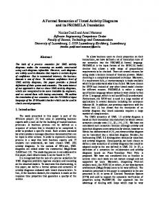
Ini B F

problem can be stated as a SCAD entailment problem: S1 |= ∃s. exec(s) ∧ (S0 @ s) ∧ T kns(F inal, s) ≥ 1? That is, is there a sequence of executable actions such that at least one token is delivered to the F inal node? Define → − a = {f ire(Ini), f ireBl (B), f ire(F ), F ire(M )}, → it can be seen that, let sa = do(− a , S0 ) 3 ,

J

S1 |= exec(sa ) ∧ (S0 @ sa ) ∧ T kns(F inal, sa ) = 1. M

M Final

Figure 1.

An activity diagram

In [4], It is shown that the reachability problem in a general K-bounded activity diagram is PSPACE-complete, that is, given a SCAD action theory Sscad , deciding Sscad ∪ Qkbound (s, p) |= Qreach (s, p) is PSPACE-complete; whereas the problem is NP-Complete if one further constraint (namely reversibility) is added. Here we show in addition that 0 Theorem 1: Given an Sscad where its nodes are free of Branch and M erge types, deciding 0

Sscad ∪ Qkbound (s, p) |= Qreach (s, p) is PSPACE-complete. Proof: (Sketch.) The same nondeterministic algorithm for the general case appeared in [4] can still be applied here to show that the problem is in PSPACE. To show that it is PSPACE-hard, we transform the PSPACE-complete Deterministic Linear Space Acceptance (DLSA) problem (see [1]) into the current problem. The proof is similar to the PSPACE-hard proof for Theorem 1 in [4], where a PSPACE-complete nondeterministic Linear Space Acceptance (NLSA) problem is applied. Here the transition function is easier as no Branch node is needed. In case a node belongs to multiple components, instead of using M erge, Branch nodes and poly-bounded duplicates of the nodes are introduced, and the proof then can be carried out in essentially the same way as the one for Theorem 1 of [4]. Example 1: A SCAD instance S1 is defined such that S1 = Df ∪ Sap ∪ Sss ∪ Suna ∪ SS0 where SS0 = {pre(Ini, B), Lpre(B, F ), RpreR(B, J), RpreL(F, J), LpreL(F, M ), preR(j, M ), pre(M, F inal), T kns(Ini, S0 ) = 2, T kns(B, S0 ) = 0, T kns(F, S0 ) = 0, T knsJl (J, S0 ) = 0, T knsJr (J, S0 ) = 0, T kns(J, S0 ) = 0,

From the fourth foundational axioms, it is obvious that S0 @ → sa . The executability of − a and T kns(F inal, sa ) = 1 can be verified by sequentially applying the four precondition axioms in Sap and the three successor state axioms in Sss . For example, P oss(f ire(Ini), S0 ), together with exec(S0 ), leads to exec(do(f ire(Ini), S0 )); whereas T kns(Ini, do(f ire(Ini), S0 )) = 1 and T kns(B, do(f ire(Ini), S0 )) = 1. Now, let → − b = {f ire(Ini), f ire(Ini), f ireBr (B), f ireBl (B), f ire(F ), F ireJ(J), F ire(M ), F ire(M )} It is obvious that T kns(F inal, sb ) = 2. The K-boundedness of S1 , meanwhile, can be stated as a SCAD entailment problem in the form: S1 |= exec(s) ⊃ T kns(p, s) ≤ 2? The proof is based on the observation that all executable sequences are with finite length. VI. S UMMARY In this paper, a graph-theoretic specification for the structural properties of activity diagrams, with adoptions of the concept of tokens in Petri-nets to model the dynamics these diagrams, is proposed. A second-order axiomatization of this semantics of UML activity diagrams called SCAD is further provided. The design of SCAD makes use of the strong correspondence between the situation s in situation calculus, which is a sequence of actions starting from the initial state S0 , and the marking M in activity diagrams, which is resulted from a sequence of node firings starting from the firing of the initial node at initial marking. R EFERENCES [1] M. Garey and D. Johnson, Computers and intractability a guide to NP-completeness. W.H. Freeman and Company, Cambridge, MA, USA (1979). [2] R. Reiter, Knowledge in Actioin: Logical foundations for describing and implementing dynamical systems, The MIT Press, 2001. [3] OMG: Unified Modeling Language (OMG UML), Superstructure, V2.1.2.,(2007). [4] X. Tan and M. Gruninger, On the computational complexity of the reachability problem in UML activity diagrams, In proceedings of the IEEE International Conference on Intelligent Computing and Intelligent Systems, Shanghai, China (2009), Vol. 2, 572–576.

T kns(M, S0 ) = 0, T kns(F inal, S0 ) = 0}

Figure 1 is its pictorial presentation. Now a reachability

3 an abbreviation for do(F ire(M ), do(f ire(F ), do(f ireBl (B), do(f ire(Ini), S0 )))).