ded design flows, notably for establishing safety and real-time requirements. ...... the sharing of concerns on many issues in life and politics, for the fun and.
Towards Component Based Design of Hybrid Systems: Safety and Stability ⋆ Werner Damm1 , Henning Dierks2 , Jens Oehlerking1 , and Amir Pnueli3 † 1
Department for Computer Science University of Oldenburg, Germany {damm,jens.oehlerking}@informatik.uni-oldenburg.de 2 Department of Electrical and Information Engineering Hamburg University of Applied Sciences, Germany 3 Computer Science Department Courant Institute of Mathematical Sciences New York University
Abstract. We propose a library based incremental design methodology for constructing hybrid controllers from a component library of models of hybrid controllers, such that global safety and stability properties are preserved. To this end, we propose hybrid interface specifications of components characterizing plant regions for which safety and stability properties are guaranteed, as well as exception mechanisms allowing safe and stability-preserving transfer of control whenever the plant evolves towards the boundary of controllable dynamics. We then propose a composition operator for constructing hybrid automata from a library of such pre-characterized components supported by compositional and automatable proofs of hybrid interface specifications.
1
Introduction
The use of component-based design approaches for embedded automotive applications has received strong momentum from the establishment of a de-facto standard for automotive component development by the Autosar consortium (see http://www.autosar.org). While the current notion of component interfaces in Autosar is rather weak, the overall strategic direction of achieving cost reductions by boosting re-use also of application components is expected to lead to an elaboration of the standard towards richer component interfaces (see e.g. [JMM08], [DMO+ 07]) providing information required for all phases of automotive embedded design flows, notably for establishing safety and real-time requirements. Related projects such as the Integrated Projects Speeds4 have provided formal contract based component interface specifications (see [JMM08]) for real-time ⋆
4
This paper reporting on joint research with Amir Pnueli is dedicated to the memory of Amir Pnueli. It has been partially supported by the German Research Council (DFG) as part of the Transregional Collaborative Research Centre “Automatic Verification and Analysis of Complex Systems” (SFB/TR 14 AVACS). IST Project 03347, see www.speeds.eu.com
and safety requirements (as in [DMO+ 07], [DPJ09]). Reflecting the significant share of control applications in embedded automotive development, this paper strives to extend this research by enabling component-based design for hybrid control applications. In particular, we propose a notion of hybrid interface specifications which is sufficiently expressive to cover the bridge between specification and implementation models of control, as elaborated below, and provide a framework for hierarchical construction of hybrid controllers supported by automatic verification tools enabling compositional verification of such interface specifications, which subsume both safety and stability properties. It is in particular (1) the need to support not only specification but as well the design phase of such systems, (2) and the need to cater for both safety and stability requirements which require extensions of previous work such as [Fre05,Fre06,Fre08] and [TPL04,HMP01] on compositional verification of hybrid systems. It follows from (1), that models which assume instantaneous reactions on mode-switching conditions, as is typically done in hybrid automata, are inadequate, since mode switching typically entails task-switching and thus comes with significant time penalties. This as well as delays in sensing and actuating the plant caused [JBS07] to propose lazy linear hybrid automata as a more realistic model of hybrid control; this model, however, is not supported by a compositional verification approach. Stauner [Sta01,Sta02] addresses the bridge between specification and design models by proposing a relaxed non-standard semantics of hybrid automata serving as specification models and proposes a systematic approach to derive discrete time design models from specification models such that this robustly refines the specification model. This approach assures that the implementation maintains safety properties, but lacks compositionality. A decompositional approach for verification of stability properties has been developed in [OT09] which constructs Lyapunov functions [Lya07] for individual modes so that there combination yields a Lyapunov function for the complete systems thus establishing stability. This approach is, however, not compositional, in that it assumes the complete system to be given as a basis for decomposition, and does not take implementation aspects into account. The key achievement of this paper is thus the development of a compositional framework for component based design of hybrid controllers taking into account realistic assumptions about reaction times. This entails the need for what we call alarms in hybrid interface specifications, which alert the environment of the component about an encountered plant dynamics, for which stability or safety are endangered, such as through trajectories violating the components assumptions on plant dynamics. Such alarms come with an escape interval, during which safety and stability are still guaranteed by the component itself, thus providing sufficient margin for task-switching. It is this paradigm shift from centralized control of mode-switching to a decentralized setting, where modes take responsibility for creating awareness about the need to perform mode-switching, 2
which is fundamental for enabling a distributed component based design of control systems. We provide a simple language in the style of Massaccio [HMP01] for the hierarchical construction of hybrid controllers, focusing in this paper on sequential composition: this allows to connect (alarm raising) outports of components through guarded transitions with inports of components, whose interface specification explicates assumptions on plant states at entry time so that safety and stability can be guaranteed, or to propagate alarms upward in the hierarchy by connecting these to outports of the enclosing system. Such port connections are annotated both with guards and jumps. We support distributed implementations of such composed components and give a distributed algorithm for resolving multiple helpful offers in alarm situations. This algorithm identifies a single helpful component, to which control is transferred, supporting in particular the delegation of control to yet unknown helpers in the environment of the composed system. Additional ingredients of interface specifications are plant safety and stability requirements, where we support both asymptotic stability as well as time bounded reachability of plant regions. We describe an approach of turning hybrid automata into a basic component supporting distributed helper identification, and employ fully automatic verification procedures [OT09] for verifying the compliance of such a component realization against its interface specification, for dynamics given as linear differential systems of equations, linear convex guards, and linear jumps, in particular relying on automatic synthesis of parameterized families of Lyapunov functions. For composed components, we give automatically verifiable verification conditions jointly ensuring, that local interface specifications augmented with auxiliary invariants such as local parameterized Lyapunov functions imply the interface specification of the composed system. These verification conditions can be seen as generating a constraint systems on parameters of local Lyapunov functions – if this constraint system is solvable, the combined system will meet its stability specification. This paper is organized as follows. The subsequent section introduces our version of hybrid automata allowing super-dense discrete time switches as well as their parallel composition. Section 3 gives syntax and semantics of hybrid interface specifications, shows how to build basic components from hybrid automata, and provides syntax and semantics for sequential composition of components, incorporating the distributed protocol for helper election. Section 4 shows how to establish the correctness of interface specifications automatically, first for basic components, and then for composed systems. We use as running example a simple automatic cruise control (ACC) system to illustrate our approach. The conclusion summarizes the key achievements and explains directions of further research.
2
Basic Definitions
In the following, we will define a hybrid automaton formalism as required for the compositional design methodology, differentiating between input variables 3
that are assumed to be outside the control of the automaton, and controllable variables that are either local, or outputs variables of the automaton. Definition 1 (Hybrid Automaton with Inputs). A hybrid automaton is a tuple H = (M, Var loc , Var in , Var out , RD , RI , RC , Φ, Θ) where 1. M is a finite set of modes, 2. Var loc , Var in and Var out are disjoint sets of local, input and output variables over R, denote Var = Var loc ∪ Var in ∪ Var out , 3. Φ is a first-order predicate over Var and a variable M , which takes values in M, describing all combinations of initial states and modes, 4. Θ is a mapping that associates with each mode m ∈ M a local invariant Θ(m), which is a quantifier-free formula over Var , 5. RD is the discrete transition relation with elements (m, Φ, A, m′ ) called tranφ,A
sitions, which are graphically represented as m −−−−→ m′ , where – m, m′ ∈ M, – φ is a first-order predicate over Var , ′ ′ – A is a first-order predicate over Var ∪ Var loc ∪ Var out specifying dis′ ′ crete updates, where Var loc and Var out are the primed variants of the variables in Var loc and Var out , D D D D R consists of two disjoint sets RU and RL . The subset RU contains the D urgent transitions, and the subset RL the lazy transitions. V • 6. RI is a first-order predicate over Var in and (Var in ) of the form v • ⊲⊳ r, where v ∈ Var in , ⊲⊳∈ {≤, =, ≥}, r ∈ R. It defines the differential inclusion modeling the evolution of the input signals. • • C 7. R over Var and (Var loc ) ∪ (Var out ) of the form V •is a first-order predicate loc out v ⊲⊳ e, where v ∈ Var ∪ Var , ⊲⊳∈ {≤, =, ≥}, and e is a real linear arithmetic expression over Var . It defines the differential inclusion modeling the continuous transition relation. The discrete update predicate will also often be implicitly defined by a sequence of assignments of the form v := e, with v ∈ Var loc ∪ Var out and e an expression over Var . We identify such a sequence of assignments with the predicate relating the pre- and post-states of its sequential execution. For graphical representation, lazy transitions will be labeled in the form φ/A, and urgent transitions ↑ φ/A, with A either in predicate or assignment notation. If a set of assignments is empty, it will be left out, meaning that all variables in Var remain unchanged upon switching. For a predicate φ, φ[A] is the result of the substitution induced by A on φ. Discrete variables may be included into hybrid automata according to our definition via an embedding of their value domain into the reals, and associating a derivative of constantly zero to them (locals and outputs). Timeouts are easily coded via explicit local timer variables with a derivative taken from {−1, 0, 1}. 4
2.1
Behavior
We now give the formal definition of runs of a hybrid automaton H capturing the evolution of modes and the real-valued variables over time. To this end, we consider the continuous time domain Time = R≥0 of non-negative reals, for the mode observable a function M : Time → M, and for the vector of variables in Var a corresponding function X : Time → R|Var | , with X(t) = [X C (t)T , X I (t)T ]T , describing for each time point t ∈ Time the current mode m and the current value of all variables in Var , respectively. Here, X C covers all variables in Var loc ∪ Var out and X I all variables in Var in . Furthermore, the vector concatenation π(t) = [M (t), X C (t)T , X I (t)T ]T describes the overall (hybrid) state of H. The order of variables in each of the two sub-vectors is fixed, but arbitrary. We identify the state vector π(t) with the corresponding valuation of the variables in M ∪ Var . For simplicity, for a predicate Ψ , we use the notation π(t) |= Ψ , if the valuation associated with π(t) fulfills Ψ . We also define a substitution based on vectors, such that the predicate Ψ [Var /X(t)] is the predicate Ψ with the variable values given by the valuation X(t) substitute the corresponding variables in Var . The vectors X C (t) and X I (t) are handled in the same manner. The time derivative of X(t) is denoted dX/dt(t) or X • (t). Definition 2 (Runs of a Hybrid Automaton). A run of a hybrid automaton H = (M, Var loc , Var in , Var out , RD , RI , RC , Φ, Θ) corresponding to a sequence of switching times (τi )i∈N ∈ Time N with τ0 = 0 ∧ ∀i ∈ N : τi ≤ τi+1 is a sequence of tuples (πi ), � � C� Mi Xi πi = , with Xi = , Xi XiI �
where Mi : [τi , τi+1 ] → M, XiC : [τi , τi+1 ] → Rn , and XiI : [τi , τi+1 ] → Rk are continuously differentiable functions such that (1) (2) (3) (4)
initial state: π0 (0) |= Φ non-Zeno: ∀t ∈ Time∃i ∈ N : t ≤ τi mode switching times: ∀i ∈ N∀t ∈ [τi , τi+1 ) : Mi (t) = M (τi ) continuous evolution: ∀i ∈ N∀t ∈ (τi , τi+1 ) : (dXiC /dt(t), Xi (t)) |= RC (Mi (τi )) (5) input evolution: ∀i ∈ N∀t ∈ Time : (dXiI /dt(t), XiI (t)) |= RI (6) invariants: ∀i ∈ N∀t ∈ Time : Xi (t) |= Θ(Mi (t)) D (7) urgency: ∀i ∈ N∀t ∈ [τi , τi+1 )∀(Mi (t), φ, A, m′ ) ∈ RU we have that Xi (t) 6|= φ. 5
(8) discrete transition firing: ∀i ∈ N : (Mi (τi+1 ) = Mi+1 (τi+1 ) ∧ Xi (τi+1 ) = Xi+1 (τi+1 )) ∨(∃(m, φ, A, m′ ) ∈ RD : Mi (τi+1 ) = m ∧ Mi+1 (τi+1 ) = m′ ∧ Xi (τi+1 ) |= φ ′
′
C ∧ |= A[Var loc ∪ Var out /Xi+1 (τi+1 ), Var /Xi (τi+1 )] I ∧ XiI (τi+1 ) = Xi+1 (τi+1 ).
Define π(t) as the πi (t), such that ∀j > i : τj > t, i.e., π(t) is the system state after all (possibly superdense) switches that occur at time t. Define X(t), M (t), X C (t) and X I (t) in the same manner. Clause (1) stipulates that a run must start with an allowed initial state. The time sequence (τi )i∈N identifies the points in time, at which mode-switches may occur, which is expressed in Clause (3). Only at those points discrete transitions (having a noticeable effect on the state) may be taken. On the other hand, it is not required that any transition fires at some point τi , which permits to cover behaviors with a finite number of discrete switches within the framework above. Our simple plant models with only one mode provide examples. As usual, we exclude non-Zeno behavior (in Clause (2)). Clauses (4) and (5) force all variables to actually obey their respective differential inclusions. Clause (6) requires, for each mode, the valuation of continuous variables to meet both local and global invariants while staying in this mode. Clause (7) forces an urgent discrete transition to fire when its trigger condition becomes true. The effect of a discrete transition is described by Clause (8). Whenever a discrete transition is taken, local and output variables may be assigned new values, obtained by evaluating the right-hand side of the respective assignment using the previous value of locals and outputs and the current values of the input. If there is no such assignment, the variable maintains its previous value, which is determined by taking the limit of the trajectory of the variable as t converges to the switching time τi+1 . Definition 3 (Reach Set). For some t ≥ 0, define a time bounded reach set reach(H, Φ, t) of hybrid automaton H from predicate Φ as the closure of {X|∃ trajectory X(·) of H, t ≥ t′ ≥ 0 : X(0) |= Φ ∧ X(t′ ) = X}. Analogously, define the unbounded reach set reach(H, Φ) of hybrid automaton H from predicate Φ as the closure of {X|∃ trajectory X(·) of H, t′ ≥ 0 : X(0) |= Φ ∧ X(t′ ) = X}. 2.2
Parallel Composition
Output variables of H1 which are at the same time input variables of H2 , and vice versa, establish communication channels with instantaneous communication. Those variables establishing communication channels remain output variables of H1 k H2 . Modes of H1 k H2 are the pairs of modes of the component automata. 6
Definition 4 (Parallel Composition). Let two hybrid automata in out D I C Hi = (Mi , Var loc i , Var i , Var i , Ri , Ri , Ri , Φi , Θi ), loc i = 1, 2 be given with Var loc 1 ∩ Var 2 = ∅. Then the parallel composition
H1 k H2 = (M, Var loc , Var in , Var out , RD , RI , RC , Φ, Θ) is given by: – – – – – – –
M = M1 × M2 , loc Var loc = Var loc 1 ∪ Var 2 , out out Var = Var 1 ∪ Var out 2 , in in in Var = (Var 1 ∪ Var 2 ) − Var out , RC ((m1 , m2 )) = R1C (m1 ) ∧ R2C (m2 ) RI = R1I ∧ R2I , D RU consists of the following transitions: D (1) ((m1 , m2 ), Φ1 , A1 , (m′1 , m2 )) for each (m1 , Φ1 , A1 , m′1 ) ∈ RU,1 , and (2) transitions of the form (1) with the role of H1 and H2 interchanged, D – RL consists of the following transitions: D , and (1) ((m1 , m2 ), Φ1 , A1 , (m′1 , m2 )) for each (m1 , Φ1 , A1 , m′1 ) ∈ RL,1 (2) transitions of the form (1) with the role of H1 and H2 interchanged, – Φ = Φ1 ∧ Φ2 , – Θ((m1 , m2 )) = Θ1 (m1 ) ∧ Θ2 (m2 ).
3
Hierarchical Controller Design
In this chapter we elaborate our approach towards component based design of hybrid controllers. We use a simplified automatic cruise control application to illustrate our design methodology and the supporting formal definitions. To simplify the exposition, we restrict ourselves to controller design for a fixed, given plant – a generalization of the approach would simply take the reference plant specification as an additional parameter of hybrid interface specifications. Formally, a plant specification is just a single-mode hybrid automaton extended with specifications of safety and stability conditions of the plant. Its input variables subsume the set of actuators, whose valuations are determined by the controller based on the current observable state of the plant as given by a valuation of its sensors. Note that we allow additional input variables to the plant – these correspond to what is typically called disturbances. The rate of change of these can be restricted by associated differential inclusions, while bounds on these can be expressed as invariance properties of the plant model. Stability requirements are expressed in terms of the interface variable of the plant and allow to specify a (convex) stability region subsuming the intended point of equilibrium. 7
Definition 5 (Plant). A plant is a hybrid automaton out D C I P = (MP , ∅, Var in P , Var P , RP , RP , RP , ΦP , ΘP )
with out – an open first-order predicate ϕsafe over Var in describing the safety P ∪ Var P P constraints of the plant, out – a convex, open first-order predicate ϕstable over Var in describing P ∪ Var P P the system stability condition.
and a set of actuator We also define a set of sensor variables S ⊆ Var Out P variables A ⊆ Var in . P Example For the simple ACC system, we restrict ourselves to a simple plant allowing to directly influence the acceleration a of the car, which is only perturbed through a disturbance s. The velocity v is observable by the controller. To simplify the discussion, we assume a fixed set point vdesired , and let v denote the difference between the actual velocity vactual and the desired velocity vdesired . The stability requirement thus specifies, that v should be close to zero, while the plant is considered to be in an unsafe state if the deviation from desired actual velocity exceeds 35m/sec. Define C I P = ({mp }, ∅, {a, s}, {v}, ∅, RP , RP , true, ΘP )
with C – RP (mP ) = (v • = sa) I – RP (mP ) = true – ΘP (mP ) = 0.975 ≤ s ≤ 1.025,
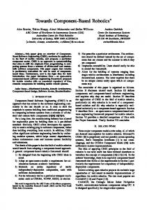
ϕsafe = (−35 < v < 35), and ϕstable = (−2 < v < 2). P P Example (cont.) To motivate our approach to component based design of hybrid controllers, consider the design of an ACC controller C controlling the above plant, given by the following specification: ϕprom ∆stable Comp. Var in Var out ϕassm • C {v} {a} −30 ≤ v ≤ 30 −2 ≤ v ≤ 1.5 300 The controller is employed in the design setting shown in Figure 1. It is required to drive the plant into its stability region within 300 seconds, for all plants states which deviate from the desired velocity vdesired by at most 30m/sec., and as long as disturbances are bounded by the plant invariant. We are also looking for an implementation which meets comfort requirements, here simplified to a maximal deceleration of 2m/sec2 , and a maximal acceleration of 1.5m/sec2 . Entry conditions shown in Figure 1 will be discussed below. 8
s
C RP (mP ) = (v • = sa) I RP (mP ) = true ΘP (mP ) = 0.975 ≤ s ≤ 1.025
v
a
ACC Controller: Picks up current velocity setpoint vdesired at activation time and controls acceleration to stabilize the plant at set point so that difference v = vactual − vdesired differs at most by 2m/s within 300 seconds, if assumptions stated by controller and plant hold. Activation port dependent on difference between vdesired and vactual at activation time.
ϕentry = β1 C
(10 ≤ v ≤ 30) = ϕentry β2 C
(−13.5 ≤ v ≤ 13.5) ϕentry = β3 C
(−30 ≤ v ≤ −10)
Fig. 1. Controller Design Setting
We envision a future design process for such embedded control applications which is supported by design libraries, whose components encapsulate “standard” control solutions. A designer would then check the hybrid interface specifications for a possible control component supporting the ACC requirement specification shown in Figure 1. Let us assume that he finds the following component specification of a component named PI . ϕprom ∆stable Comp. Var in Var out ϕassm • PI {v} {a} −15 ≤ v ≤ 15 −1.4 ≤ v ≤ 1.4 300 This component is offering a convergence time to the stability region which matches the specifications, although only for a restricted subspace of the plant. It employs an acceleration which matches those of the specification, and thus altogether looks like a good starting point for the controller design, if we can extend the scope of the controllable plant region with some “glue” control. This takes us to a central point of our design methodology. Since we are addressing, as in AUTOSAR, distributed control applications, where different subcomponents of controllers are running on different electronic control units, we can no longer as in hybrid automata rely on a centralized control structure 9
ensuring mode switching. Instead, in this distributed setting, it becomes the duty of components to raise an alarm if the dynamics of the plant is evolving in an unforeseen way (such as through differences between the idealized plant model and the actual controlled plant, e.g., unmodeled disturbances). This must happen in time to allow a control component capable of addressing the critical dynamics to take control. We thus extend our interface concept by allowing the declaration of possibly multiple outports encapsulating possibly different types of dynamics raising alarms. Such outport specifications signal the plant state causing the alarm, and provide time-guarantees for maintaining stability and safety for a rescue period, thus providing a time-window in which the switch of control can be initiated. To support a distributed agreement protocol for the selection of the as it were “helper component”, there is a persistency requirement on such alarm signals. They also exhibit the plant state at the latest allowable time for control-switch, as determined by the duration of the rescue period and the cost for control switching, which we assume to be given as a design parameter τ . Example (cont.) For the PI control component, we have two sources of endangering the component’s promises in maintaining safety and stability, in that the vehicle could become either significantly slower or faster than the desired speed, as catered for in the following two outport specifications: µα ∆α ϕexit Outport Comp. ϕalarmOn α α 1 αPI PI v ≥ 14 0.006 0.01 13.9 ≤ v ≤ 14.1 2 αPI PI v ≤ −14 0.006 0.01 −14.1 ≤ v ≤ −13.9 By way of returning to our design scenario, let us assume that the design library offers a component which addresses traffic situations, where the actual velocity is significantly below the desired velocity, a simple acceleration component ACCELERATE with a still acceptable constant acceleration, which could recover from such plant states and force the plant into regions allowing a more fine-grained control, as exemplified below. Var in Var out ϕassm ϕprom ∆stable Comp. ACCELERATE {v} {a} −30 ≤ v ≤ −5 v • = 1.5 300 The ACCELERATE component raises an alarm if its assumptions are endangered: Outport Comp. ϕalarmOn µα ∆α ϕexit α α αACCELERATE ACCELERATE v ≥ −6 0.005 0.01 v ≥ −6 Intuitively, the combination of the ACCELERATE component with the PI component yields a more robust system, in that safety and stability are now guaranteed for a larger plant region. 10
We have now motivated most concepts occurring in a hybrid interface specification. The one remaining concept is that of inports: these serve to activate components resp. resume execution of components, under specified entry conditions, which jointly cover the assumptions on plant states for which this component guarantees safety and stability. Each inport specification defines as well a time-window in which it promises to respond to rescue requests arriving at this port. Example (cont.) The PI component offers a single inport Alarm requests are answered within a time window of 0.0025 seconds. ϕentry Inport Comp. λβ β βPI PI 0.0025 −13.5 ≤ v ≤ 13.5 To summarize, a hybrid interface specification for a given plant model P consists of – a static interface definition of real-valued data interface variables and boolean control variables, – specification of inports and outports, which in addition to the concepts elaborated in the example also define control signals used for distributed agreement in context-switching, as elaborated below, – a specification of the plant states for which this component guarantees safety, stability, and promises, – promises on the rate of change of out-variables, – a maximal time to convergence to the plant stability region. Definition 6 (Component Interface Specification). A component C associated with a plant P is described by an externally visible interface SPEC C consisting of: in – Var in C , a set of real valued input variables with S ⊆ Var C , out – Var C , a set of real valued output variables which is disjoint from Var in C and with A ⊆ Var out , C in out – CC = {suspend C } ∪ {cβ , start β | β ∈ Ain C } ∪ {take α | α ∈ AC }, a set of binary control inputs, out out – CC = {active C , fail C } ∪ {take β | β ∈ Ain C } ∪ {bα , switch α | α ∈ AC }, a set of binary control outputs, – a set Ain C of incoming ports (“inports”) given as tuples
β = (cβ , λβ , take β , start β , ϕentry ), β in out in where cβ ∈ CC , λβ > 0, take β ∈ CC , start β ∈ CC , and ϕentry is a β out , ∪ Var first-order predicate over Var in C C – a set Aout C of outgoing ports (“outports”) given as tuples
α = (bα , ϕalarm , µα , ∆α , take α , switch α , ϕexit α α ), out out where bα ∈ CC , ϕalarm is a closed first-order predicate over Var in C ∪Var C , α in out exit µα > 0, ∆α > 0, take α ∈ CC , switch α ∈ CC , and ϕα is a first-order out predicate over Var in C ∪ Var C ,
11
•
•
out out – ϕprom , a first-order predicate over Var in ∪ Var in C ∪ Var C C ∪ Var C , C out in assm – ϕC , a first-order predicate over Var C ∪ Var C , – ∆stable > 0 is a time after which the system is required to converge to ϕstable . C P W entry entry In the rest of this paper we use ϕC to abbreviate β∈Ain ϕβ . C
Definition 7 (Switch Time). Define a global variable 0 < τ ∈ R, representing the maximum time needed for a component switch.
We will now discuss how to build controllers hierarchically, and use the running ACC controller design to illustrate the key underlying concepts and issues. Example (cont.) Var in Var out ϕassm ϕprom ∆stable Comp. • PI {v} {a} −15 ≤ v ≤ 15 −1.4 ≤ v ≤ 1.4 300 ACCELERATE {v} {a} −30 ≤ v ≤ −5 v • = 1.5 300 Outport 1 αPI 2 αPI αACCELERATE
Comp. PI PI ACCELERATE
ϕalarmOn α v ≥ 14 v ≤ −14 v ≥ −6
µα ∆α ϕexit α 0.006 0.01 13.9 ≤ v ≤ 14.1 0.006 0.01 −14.1 ≤ v ≤ −13.9 0.005 0.01 v ≥ −6
Comp. λβ ϕentry Inport β βPI PI 0.0025 −13.5 ≤ v ≤ 13.5 βACCELERATE ACCELERATE 0.0025 −30 ≤ v ≤ −10 We compose the PI and ACCELERATE components as follows: – an alarm raised by ACCELERATE is forwarded to the inport of the PI component, – an alarm raised by the PI component of type “actual speed is too slow to be handled by PI component” is forwarded to the inport of the PI component. Note that such a composition leaves unspecified, how to handle plant dynamics, in which the current speed is much too fast in relation to the desired speed for the PI component to maintain stability. In general, the composition of two components then yields a composed component, whose outports must cater for alarms which are not handled internally. Figure 2 gives an informal description of the composition of the PI component and the ACCELERATE component. We can now perform a what in industrial design processes is typically referred to as a virtual integration test: – Is the plant state at context switch time as given by the exit predicate of the outport compatible with the plant state required by the connected inport? – Does the inport have sufficient time to take a decision on whether it is willing to accept the alarm? To this end we compare the promised minimal stability period µα of outport, as expressed by the λβ which provides an upper bound for the inport to reply to incoming alarms. 12
1 βC 2
αC2 βPI
αACCELERATE
1 αPI
PI
ACCELERATE
2 αPI
2 βC 2
βACCELERATE
Fig. 2. Interconnection of ACCELERATE and PI
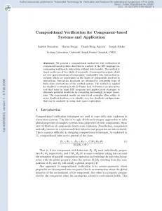
Having successfully carried out the virtual integration test, we can now either derive a component interface specification for the composed system C2 , by propagating information derived from local specifications towards the boundary of the system, or check, whether an a priori given specification of the composed system C2 is derivable from local specifications. This reasoning will be formalized in Section 4 on verification of hierarchical component based controller designs. The key property conspicuous already in our simple example is, that this reasoning is completely independent of the actual implementation of the subsystems. Indeed, the PI component might itself be composed of several subsystems, or be given as a what we call basic component: both the virtual integration test as well as compliance of the composed system to an interface specification of the composed system is purely based on component interface specifications. Industrial jargon uses the term grey box view to refer to schematics of a composed system as in Figure 2, where only the interface specifications of subsystem as well as their interconnection via ports are known. In contrast, a white box view of a composed system would also make visible the internal realization of the subsystems, across all levels of hierarchy. We will use a white box view on composed systems to define their semantics, and a grey box view in Section 4 for compositional verification of such systems. As in the ACC example, components of a composed system offer different capabilities in establishing safety and stability requirements of one and the same plant. The formal definition of what we call the transition composition of components exhibits the following aspects. – Alarms may be either be handled locally of forwarded to a yet unknown environment. – We allow for multiple helpers, and offer guards on port connections to filter propagation of alarms. – On the path to local helpers, interface variables of the entered component may be updated (thus motivating the usage of term transition composition). – Statically it must be possible to have at least one feasible path to ask for help: the disjunction of all guard conditions related to a single outport must be a tautology. 13
In Def. 6 we defined the externally visible interface of a component C. Components may also use local variables internally and we denote the set of these variables with Var loc C . In the following definition we use C(α) (resp. C(β)) to denote the component C the port α (resp. β) belongs to, i.e. α ∈ Aout (resp. C β ∈ Ain ). C Definition 8 (Transition Composition of Components). Let C be a component and let {C1 , . . . Cn } be a finite set of basic or composed components with in – Var in C = Var Ci for all i, out – Var out C = Var Ci for all i, in in out – all ACi , ACi , as well as Aout C and AC are disjoint. S loc We define Var loc C := i Var Ci and call C a transition composition of the components C1 , . . . Cn with port connection (P, Q) (we use S(P,Q) (C1 , . . . , Cn ) to denote it) iff
(a) P is given as a set of tuples describing transitions of the form (α, {(β1 , g1 , A1 ), . . . , (βk , gk , Ak )}, {(α1 , g1′ ), . . . , (αl , gl′ )}), with S – α ∈ i Aout Ci , – k, l ≥S0, k + l > 0, – βi ∈ i Ain Ci with βi 6= βj for all i 6= j ∈ {1, . . . , k}, – αi ∈ Aout C with αi 6= αj for all i 6= j ∈ {1, . . . , l}, out loc – gi and gi′ are first-order predicates over Var in C ∪ Var C ∪ Var C , such W W ′ that for each tuple i gi ∨ i gi holds, – for all (α, {(β1 , g1 , A1 ), . . . , (βk , gk , Ak )}, {(α1 , g1′ ), . . . , (αl , gl′ )}) ∈ P, α belongs to a different component than all βi (no loops, C(α) 6= C(βi )), in – Ai is a set of assignments for Var in C(αi ) \ S depending on Var C(α) ∪ out Var C(α) , – for all α, there exists exactly one tuple (α, S1 , S2 ) ∈ P (each outgoing alarm is connected to exactly one family of incoming alarms). (b) The second component Q of the port connection is a totally defined mapping S in from Ain to A . C i Ci
This definition connects the components C1 , . . . , Cn that have equal Var in and Var out and the result is a component C. The composition C and its components C1 , . . . , Cn carry control in- and outputs that are connected appropriately in the above definition. A tuple p = (α, {(β1 , g1 , A1 ), . . . , (βk , gk , Ak )}, {(α1 , g1′ ), . . . , (αl , gl′ )}), connects an outport α of a component Ci with some inports βi of the other components and with some outports αj of the composition C. The idea is that the outgoing signal of α is forwarded to the βi ’s and αj ’s such that each receiver of this signal is able to respond appropriately and to take over. However, this action 14
requires that the corresponding entry condition of the activated component is met. Hence, the composition must be able to ensure that and therefore p adds a guard for each receiving port. Moreover, it adds assignments to each connection between α and an inport βi of another component. This allows for setting nonsensor variables as required. The above definition lists sanity conditions for a port connection p. There must be at least one receiver, no inport is used twice as receiver, no outport is used twice as receiver, there is always at least one of the guards satisfied, and there are no loops, i.e., no component receives its own outgoing signal. All these tuples are collected in the set P and for each outport that appears in C1 , . . . , Cn we have exactly one p ∈ P describing the receivers of this signal. The inports of the composition are receiving signals and therefore this information must be forwarded to some inports of its components. In the above definition this is done by an one-to-one mapping Q. In Fig. 3 an example for transition composition is given. It consists of a composition SP,Q (A, B) of A and B which is then composed with C. We now return to the role of the control signals in component interface specifications. Consider the transition composition of components A, B, and C in Figure 3, and assume a distributed implementation, where A and B are allocated on ecu1 , and C is allocated on ecu2 , and consider an alarm raised by component B at outport α2 . We will now informally describe a distributed agreement protocol, ensuring that all ECUs agree on the component to handle the alarm, called distributed identification of helpers. The challenge arises from the distributed execution, and the possibility of multiple helpers. Much as in distributed cache coherency protocols, we need to enforce a serialization point so as to avoid race conditions leading to inconsistent states, where say both A and C believe to be the chosen helper. We describe the protocol informally using the sequence chart given in Figure 4. Formally, we will define with each component wrapper automata jointly implementing the protocol. Such wrapper automata are constructed both for outports – such as H3 (B) – , for port connections – such as HP and HP ′ – , and for inports, such as Hβ1 (A) and Hβ2 (C) in Figure 4. The protocol is initiated from the basic component B: it raises an alarm at its outport α2 , which causes the control signal bα2 associated with this outport to be generated. There are two levels of hierarchy enclosing component B, each specifying through port connections potential helper components. From the inner hierarchy, we see that either the alarm can be handled locally – this is reflected by requesting help from import β1 of component A through generation of the control signal cβ1 associated with this inport, or externally, which is represented by generating an alarm at the outport α4 of the composed system, represented by setting its control signal to 1. This is handled by the wrapper automaton HP for this port connection running on ecu1 . We now have two independent message flows – in which the generated control signals are propagated either locally within ecu1 or externally to ecu2 (typically with different arrival times). The local flow will lead to a response of component 15
P Var out P
Var in P
C β3 α 3
true
true β5
true
α5
α4 true
β4
¬g
α1 A β1
α2 β 2
g
B SP,Q (A, B) SP ′ ,Q′ (C, SP,Q (A, B)) � � (α1 , ∅, {(α5 , true)}), Bottom: SP,Q (A, B) with P = and Q(β4 ) = β2 . (α2 , {(β1 , g)}, {(α4 , ¬g)}) (α3 , {(β4 , true, ∅)}, ∅), ′ (α4 , {(β3 , true, ∅)}, ∅), and Overall: SP ′ ,Q′ (C, SP,Q (A, B)) with P = (α5 , {(β3 , true, ∅)}, ∅) Q′ (β5 ) = β4 . Fig. 3. An example for a composition
A through its inport β1 to be ready for taking over, as indicated by setting the associated control signal take β1 . The external flow will lead to the generation of a help request (control signal cβ3 ) to the inport of component C, generated by a wrapper automaton interpreting the port connection P ′ of the outer hierarchy level. Component C will indicate its readiness to accept the alarm by setting the control variable take β3 . Outports of composed components act as a proxy for the environment, in that the existence of at least one helper component in the environment of the sequential composition of A and B, such as component C, is then communicated internally, with the outport behaving on behalf of an inport of such an environment component. Thus outport α4 generates take α4 in response to receiving take β3 . The protocol automaton HP associated with port connection P will for each offer for help consult guards of port connections, and only register this offer for help, if the guard condition is true. Note that this condition might change dynamically; HP thus constantly monitors guard conditions associated 16
H3 (B)
Hβ1 (A)
HP
HP ′
Hβ3 (C)
bα2 := 1 cβ1 := 1 bα4 := 1 cβ3 := 1 take β1 := 1 g
take β3 := 1 take α4 := 1
true
¬g
take α2 := 1 bα2 := 0 switch α2 := 1 ?
switch α4 := 1 start β3 := 1 start β1 := 1
The diagram represents the sequence of signals that are set as a consequence of setting bα2 . In this example there is a race between the inport β1 and β3 . As soon as a take is observed by HP , the automaton forwards this to B. When the switch signal is set, the automaton HP decides by considering the guards who takes over. Fig. 4. Sequence of communications when bα2 is set
with registered helpers, and removes registration if associated guards become false. The protocol will ensure that helpers maintain their readiness for help, until finally a helper is selected. This selection occurs as follows. As soon as there is at least one registered helper, HP signals this information to the outport α2 which raised the alarm, by setting its in-control signal take α2 . If this signal arrives prior to the expiration of the rescue period, taking into account the time needed for context switching, the context switch is initiated by the declaration on part of B to now delegate control to some helper, through setting switch α2 . HP , the single point of serialization in this protocol, consults upon receiving switch α2 the list of registered helpers, and nondeterministically picks one of these. In the example above, depending on the guard condition g at helper selection time, this can either be the local helper A, in which case it passes control to helper A by setting its in-control-signal start β1 , or some external helper, in which case HP 17
delegates control to the helper in the environment of the sequential composition of A and B by setting switch α4 . In the former case, the environment would be informed, that a helper has been found by resetting bα4 , which in turn would cause component C to withdraw its offer. In the latter case, bα2 is withdrawn, and any local helper such as B will withdraw its offer. We note that watchdogs are employed in various places in the protocol to monitor the deadline for context switching, as defined by the rescue period of the alarm raising outport and the time needed for context switching. In case such a watchdog expires, a failure state is reached. We now complement the definition of hybrid component interfaces and transition composition of components with three steps addressing in particular their semantic foundation. We will first show how to systematically derive basic components from hybrid automata and define the induced semantics of basic components. We then turn to the semantics of transition composition, which is derived inductively from the semantics of its components and automata implementing the distributed helper agreement protocol. Finally, we define the satisfaction relation between component implementations and hybrid interface specifications. The section is wrapped up by completing the construction of the automatic cruise controller. Definition 9 (Hybrid Automaton for a Basic Component). Let H = (M, Var loc , Var in , Var out , RD , RC , RI , Φ, Θ) be a hybrid automaton with disjoint Var loc , Var in , and Var out . Define – for each incoming port β in Ain , a first-order predicate Φβ on Var loc , describing admissible initial values for the local variables when start β is received, – for each incoming port β in Ain , an initial mode mβ ∈ M. We call H an admissible hybrid automaton for a basic component C associated with a plant P if and only if – – – –
in Var in C = Var , out out Var C = W Var , Φ =⇒ β∈Ain Φβ , and VC ϕassm =⇒ m∈M ΘC (m) C
In this case we use HC to denote the hybrid automaton H of the basic component C. Now consider an admissible hybrid automaton for a given interface specification. From an implementation perspective, we now wrap the code generated from this hybrid automaton with code supporting suspension and activation, an automaton providing a single point of serialization for all outports, and automata implementing the distributed agreement protocol requirements for inports. Cast as a formal definition of the semantics of basic components, this can be formalized as a parallel composition of a relaxation of the hybrid automata 18
providing the component implementation, and as timed automata implementing the distributed agreement protocol. This relaxation of the admissible hybrid automaton enforces no constraints on the input and output variables whenever the component is inactive. Definition 10 (Semantics of a Basic Component). Let H = (M, Var loc , Var in , Var out , RD , RC , RI , Φ, Θ) be a hybrid automaton, and C a basic component such that H is admissible for C. The semantics [[C]] of C is the parallel composition of hybrid automata � � Hβ , IC = H1 k H2 k H3 k kβ∈Ain C
which are defined as follows.
– H1 is a hybrid automaton that is basically H but augmented with a mode minact for inactivity and a mode mfailed for failures: out H1 = (M ∪ {minact , mfailed },Var loc , Var in ∪ {fail C }, H1 , Var D C RH , RH , true, Φ ∧ M = minact , ΘH1 ), 1 1
where • minact , mfailed ∈ / M, in • Var in ∪ {active C } ∪ {start β | β ∈ Ain H1 = Var C }, • D D = RU ∪ {(m, active C = 0, ∅, minact ) | m ∈ M} RU,H 1
ϕentry , β
∪ {(minact , active C = 1 ∧ start β ∧ ^ (v ′ = v), mβ ) | β ∈ Ain Φ′β ∧ C },
(1) (2)
v∈Var out
∪ {(minact , active C = 1 ∧ start β ∧ ¬ϕentry , β
(3)
fail C := 1, mfailed ) | β ∈ Ain C }, where Φ′β is Φβ with every variable primed, D D = RL • RL,H 1 C C (minact ) = true, • RH1 (m) = RC (m), if m ∈ M, and RH 1 • ΘH1 (m) = Θ(m), if m ∈ M, and ΘH1 (minact ) = true, – Automaton H2 ensures that the variables active C and fail C are only changed by discrete transitions (Fig. 5). It also reacts to suspend C signals by deactivating the component. – The hybrid automaton H3 handles all outgoing ports. It is defined as follows: H3 = (M3 , V3loc , V3in , V3out , R3D , R3C , R3I , Φ3 , Θ3 ) 19
with � out � out M3 = 2AC × 2AC ∪ {F ail},
(4)
V3loc = {tα | α ∈ Aout C },
out out V3in = {active C } ∪ Var in C ∪ Var C ∪ {take α | α ∈ AC },
V3out = {fail C } ∪ {bα , switch α | α ∈ Aout C }, D RU,3 = {((X, Y ), ϕalarm ∧ active C , bα := 1, tα := 0, α
(5)
(X ∪ {α}, Y )) | α ∈ / X ∪Y} //Alarm α is set ∪ {((X, Y ), tα ≥ α, fail C := 1, F ail) | α ∈ X} // Failure: alarm α has exceeded the maximum duration
(6)
∪ {((X, Y ), take α ∧ tα < ∆α − τ, bα := 0, tα := 0, (X \ {α}, Y ∪ {α})) | α ∈ X \ Y }
(7)
//Alarm α is reset because of a take ∪ {((X, Y ), tα = 0, V3out
(8)
V3loc
switch α := 1, ∀v ∈ ∪ \ {switch α } : v := 0, (∅, ∅)) | α ∈ Y } //A switch α is set because of a previous take α D RL,3 = {((X, Y ), µα ≤ tα < ∆α ∧ ¬ϕalarm , bα := 0, tα := 0, α
(9)
(X \ {α}, Y )) | α ∈ X} //Alarm α can be reset R3C (v) = 0 for all v ∈ V3out R3C (v) = 1 for all v ∈ V3loc R3I = true Φ3 = (M = (∅, ∅) ∧
^
v = 0)
v∈V3out ∪V3loc
Θ3 = true
(10)
– The automaton Hβ for an incoming port β = (cβ , λβ , take β , start β ) ∈ Ain C is given in Fig. 6. On H1 of the semantics of a basic component: The purpose of H1 is to add the intended control strategy of H into the semantics. However, we have to augment this by additional locations and some transitions in order to satisfy SPEC C . The automaton H1 behaves like H except for the case that active C becomes false. In this case H1 switches by (1) from an arbitrary location to the additional location minact which stands for inactivity. As soon as H1 discovers a rising edge of active C together with start β the automaton fires transition (2) because 20
active C = 0 fail C = 0
active C • = 0 fail C • = 0
↑ suspend C = 1/ active C := 0
Fig. 5. Automaton H2
cβ = 1 ∧ tβ > 0/take β := 1, tβ := 0 take β = 0
↑ cβ = 1/tβ := 0
idle tβ • = 0 take β • = 0
↑ cβ = 0
alert tβ • = 1 take β • = 0
↑ tβ ≥ λβ ∧ tβ > 0 ∧ cβ = 1/ offer take β := 1, tβ := 0 tβ • = 0 take β • = 0
↑ ¬start β ∧ ¬cβ /take β := 0
tβ ≤ τ ∧ ϕentry β /active C := 1
/active C := 1 ↑ tβ = τ ∧ ϕentry β activate tβ • = 1 take β • = 0
↑ start β ∧ ¬cβ /take β := 0
↑ tβ = τ ∧ ¬ϕentry /fail C := 1 β fail tβ • = 0 take β • = 0
Fig. 6. Automaton Hβ
it knows that is activated again via the incoming port β. The assignment that belongs to this transition keeps all variables of Var out stable but executes the C assignments Φβ given by the definition of β when switching to mβ . Note that both Φβ and mβ were given in Def. 9. However, if the activation takes place while the entry condition ϕentry is not given, then H1 switches to a location β mfailed and sets fail C . On H3 of the semantics of a basic component: The purpose of H3 is to manage the outgoing alarm signals bα . To this end H3 has locations defined in (4) of 21
out
the form (X, Y ) with X, Y ∈ 2AC with only one exception needed for failures. The idea of a location (X, Y ) is that for all α ∈ X the corresponding signal bα is currently set. If α ∈ Y then this means that the component has observed a rising edge of take α . The transitions are defined to keep these invariants. In is satisfied while C is active. With (5) the signal bα is set as soon as ϕalarm α this transition a timer tα is reset to observe whether a take α is set in time or ϕalarm becomes false in time. If this is not the case, then the transitions in (6) α will switch to the exceptional failure state and will set fail C . The transitions (7) are fired provided that a take α signal arrives in time, i.e. it arrives τ time units before the component is signaling bα for ∆α time units. This transition moves α from the X set into the Y set. For an α being in Y the automaton has to react within 0 time units by setting switch α as given in (8). If bα is set for at least µα time units the automaton is able to reset this signal provided that ϕalarm is α not satisfied anymore (9). Note that these transitions are not urgent, hence the automaton is not forced to do this if the transition is enabled. On Hβ of the semantics of a basic component: The purpose of Hβ is to handle incoming requests at inport β. Initially it waits in idle until a rising edge of cβ is observed. This enforces a transition to alert where the automaton might remain for a while. Due to the timer tβ and the urgent transition with guard tβ ≥ λβ the automaton sets take β after at most λβ time units and switches to state offer . A prerequisite is that the cβ is still set, otherwise Hβ moves back to idle. In offer it waits for a falling edge of cβ . If this happens with start β being set, the automaton switches to activate and activates the component after at most τ seconds. Otherwise, i.e. start β is not set, the automaton proceeds to idle without activating the component. In case that the activation must take place (τ seconds elapsed) and the entry condition ϕentry is not true, the automaton C sets fail . We can now define the semantics of the transition composition of components C1 , . . . , Cn , where in taking a white box view we assume as given the semantics [[Cj ]] of the components. The semantics is defined in terms of the parallel composition of the hybrid automata representing the semantics of its components, and three timed automata which define activation and failure of the composed systems in terms of the status of its components, interpret the connection of inports of the composed system to local inports in propagating control signals outsidein, and interpret all port connections for all local outports to implement the distributed helper identification protocol. Note that control signals ensure that there is always at most one active component inside a transition composition of components. Definition 11 (Semantics of a Transition Composition). Let C be a component obtained by a transition composition of the components C1 , . . . Cn with port connection (P, Q). The semantics [[C]] of C is the parallel composition of hybrid automata ! n IC = [[Ci ]] k HT k HP k HQ i
22
Hβ3 (C) β3 HP ′
¬g
Hβ1 (A) β1
true α4
g
α2 HP
H3 (B)
SP,Q (A, B) SP ′ ,Q′ (C, SP,Q (A, B))
Fig. 7. Semantics: Automata involved for α2
with the following components.
– HT is a hybrid automaton that handles the reactions to suspend C , start β , and F ailCi appropriately:
MT ={inactive, active, failed } VTloc =∅, VTin ={start β | β ∈ Ain C } ∪ {active Ci , fail Ci | i ∈ {1, . . . , n}} ∪ {suspend C } VTout
={suspend Ci | i ∈ {1, . . . , n}} ∪ {active C , fail C } 23
D RU,T ={(m, fail Ci , fail C := 1, failed ) | i ∈ {1, . . . , n}, m ∈ MT }
// A component failed, hence the composition fails. ∪{(m, suspend C , active C := 0, suspend C1 := 1, . . . , suspend Cn := 1, inactive) | m ∈ MT \ {failed }} // Suspend is forwarded to all components. ∪{(inactive, ¬suspend C , suspend C1 := 0, . . . , suspend Cn := 0, inactive)} // Reset of suspend is forwarded to all components. ∪{(inactive, start β ∧ ϕentry , active C := 1, active)} β // A start β activates the composition C. ∪{(inactive, start β ∧ ¬ϕentry , fail C := 1, failed )} β // A start β without meeting the entry condition. ∪{(active, active Ci , suspend C1 := 0, . . . , suspend Ci−1 := 0, suspend Ci+1 := 0, . . . , suspend Cn := 0, active)} // When a Ci becomes active, all others are suspended. D RL,T =∅
RTC (v) =0 for all v ∈ VTout ∪ VTloc RTI =true ΦT =(M = inactive ∧
^
v = 0)
v∈VTout ∪VTloc
ΘT =true – HQ is a hybrid automaton that implements the invariant ∀β ∈ Ain C : (cβ ←→ cQ(β) )
– Let Asrc =
S
i
Aout Ci
∧(take Q(β) ←→ take β ) ∧(start β ←→ start Q(β) ) S and Adst = i Ain Ci . We set
D C I HP = (MP , VPloc , VPin , VPout , RP , RP , RP , Φ P , ΘP )
with MP =2A VPloc
src
× 2A
=∅, 24
src
×(Adst ∪Aout C )
,
out src VPin =Var in } C ∪ Var C ∪ {bα , switch α | α ∈ A
∪ {take β | β ∈ Adst } ∪ {take α | α ∈ Aout C }, VPout ={cβ , start β | β ∈ Adst } ∪ {bα , switch α | α ∈ Aout C } D RU,P
∪ {take α | α ∈ Asrc }, [ D D RU,P (p) where RU,P (p) is defined in Fig. 8 = p∈P
D RL,P C RP (v) I RP
=∅
=0 for all v ∈ VPout ∪ VPloc =true
ΦP =(M = (∅, ∅) ∧
^
v = 0)
v∈VPout ∪VPloc
ΘP =true In summary, the semantics of a transition composition is the parallel composition of semantics of its components together with three additional hybrid automata HT , HP and HQ . The automaton HT implements the following properties: – Whenever a fail Ci of a component occurs this leads to a fail C signal. There is no way to reset fail C . – Whenever a start β signal is given then the composition is activated provided that the entry condition ϕentry is met. Otherwise HC produces a fail C signal. β – It observes active Ci signals of the components and provide suspend Cj signals to all j 6= i. This is needed in case of an internal take over situation. In the case of HQ this automaton just implements invariants over the variables. As the details of this automaton is straightforward they are not given here. The invariants implemented are also fairly obvious. Not trivial is the construction of HP . Its purpose is to implement the correct handling of the outgoing signals of the components. A location of HP is a pair (X, Y ), where – X contains all α ∈ Asrc which are currently set. The set Asrc is the union of all outport of the components C1 , . . . , Cn . – Y is set containing pairs (α, βi ) or (α, αj ) where α ∈ Asrc , βi is an inport of a component and αj is an outport of the composition C. A pair being in Y stands for the information that α is set and a take from βi resp. αj has been set. The transitions of HP are given in Fig. 8 and they are implementing the invariants for the locations given above. Whenever bα becomes true, then α is added to the X set (11). Moreover, this transition forwards this signal to all connected inport and outport. As soon as a take is received from there the corresponding pair is added to the Y set (12–13). To do so, it is required that the given guard gi resp. gj′ are satisfied. The transitions (14–17) handle the various cases that 25
For a tuple p = (α, {(β1 , g1 , A1 ), . . . , (βk , gk , Ak )}, {(α1 , g1′ ), . . . , (αl , gl′ )}) ∈ P D we set RU,P (p) to
{((X, Y ), bα , cβ1 := 1, . . . , cβk := 1, bα1 := 1, . . . , bαl := 1,
(11)
(X ∪ {α}, Y )) | α ∈ / X} //Alarm α is set, all connected βi , αj are set ∪{((X, Y ), take βi ∧ gi , take α := 1, (X, Y ∪ {(α, βi )})) | α ∈ X, (α, βi ) ∈ / Y}
(12)
//There is a take from a connected βi which is forwarded ∪{((X, Y ), take αj ∧ gj′ , take α := 1, (X, Y ∪ {(α, αj )})) | α ∈ X, (α, αj ) ∈ / Y}
(13)
//There is a take from a connected αj which is forwarded ∪{((X, Y ), ¬(take βi ∧ gi ), take α := 1,
(14)
(X, Y \ {(α, βi )})) | α ∈ X, (α, βi ) ∈ Y, ∃γ : (α, γ) ∈ Y \ {(α, βi )} //βi is not able to take over anymore, but an alternative is left ∪{((X, Y ), ¬(take βi ∧ gi ), take α := 0,
(15)
(X, Y \ {(α, βi )})) | α ∈ X, (α, βi ) ∈ Y, ¬(∃γ : (α, γ) ∈ Y \ {(α, βi ))} //βi is not able to take over anymore and no alternative is left ∪{((X, Y ), ¬(take αi ∧ gi′ ), take α := 1,
(16)
(X, Y \ {(α, αj )})) | α ∈ X, (α, αj ) ∈ Y, ∃γ : (α, γ) ∈ Y \ {(α, αj )} //αj is not able to take over anymore, but an alternative is left ∪{((X, Y ), ¬(take αi ∧ gi′ ), take α := 0,
(17)
(X, Y \ {(α, αj )})) | α ∈ X, (α, αj ) ∈ Y, ¬(∃γ : (α, γ) ∈ Y \ {(α, αj ))} //αj is not able to take over anymore and no alternative is left ∪{((X, Y ), switch α , start βi := 1, Ai , RESET (Var out P \ {βi }),
(18)
(∅, ∅)) | α ∈ X, (α, βi ) ∈ Y ))} //There is a switch which is forwarded to a connected β ∪{((X, Y ), switch α , switch αj := 1, RESET (Var out P \ {αj }), (∅, ∅)) | α ∈ X, (α, αj ) ∈ Y ))} //There is a switch which is forwarded to a connected α where RESET ({v1 , . . . , vM }) stands for v1 := 0, . . . , vM := 0. Fig. 8. Urgent transitions for a p ∈ P
26
(19)
either a guard becomes not satisfied or the corresponding take signal was reset. They have to distinguish the case whether the take α signal has to be reset or not. If a (α, βi ) or (α, αj ) must be removed from the Y set, then the question is whether an alternative is left. If it is, the take α can remain set, otherwise it must be reset. As soon as a switch α occurs the HP automaton has to react without delay due to the transitions (18–19). They select a switch αj or start βi signal where (α, αj ) resp. (α, βi ) must be in the current Y set. This ensures that the corresponding guard is currently satisfied. In case of start βi the assignments are also executed. Note that the selection is done nondeterministically if more than one option is available. However, the reaction to a switch α happens without delay because the transitions are defined as being urgent. Definition 12 (Semantics of a Closed Loop). The semantics of a closed loop consisting of a component C and a plant P is defined as [[C k P ]] := [[C]] k P .
αBRAKE
BRAKE
βBRAKE
1 βC
2 βC 1 βC 2
αC2 βPI
αACCELERATE
1 αPI
PI
ACCELERATE
2 αPI
2 βC 2
βACCELERATE
3 βC
Fig. 9. Interconnection Structure for the ACC Example
We now complete the design of the ACC controller. Example (cont.) We complete the design by adding a BRAKE component to cater for the so far unserved alarm of the PI controller for plant situations where the actual velocity is much higher than the desired velocity, and arrive at the hierarchical composition depicted in Figure 9. 27
Comp. C BRAKE C2 PI ACCELERATE
Var in {v} {v} {v} {v} {v}
Var out {a} {a} {a} {a} {a}
Var loc {x} ∅ {x} {x} ∅
ϕassm −30 ≤ v ≤ 30 5 ≤ v ≤ 30 −30 ≤ v ≤ 15 −15 ≤ v ≤ 15 −30 ≤ v ≤ −5
ϕprom −2 ≤ v • ≤ 1.5 v • = −2 −1.4 ≤ v • ≤ 1.5 −1.4 ≤ v • ≤ 1.4 v • = 1.5
∆stable 300 300 300 300 300
Table 1. Component Interfaces (and local variables) for ACC Example
Outport αBRAKE αC2 1 αP I 2 αP I αACCELERATE
Comp. BRAKE C2 PI PI ACCELERATE
ϕalarmOn α v≤6 v ≥ 14 v ≥ 14 v ≤ −14 v ≥ −6
µα 0.005 0.006 0.006 0.006 0.005
∆α 0.01 0.01 0.01 0.01 0.01
ϕexit α v≤6 13.9 ≤ v ≤ 14.1 13.9 ≤ v ≤ 14.1 −14.1 ≤ v ≤ −13.9 v ≥ −6
Table 2. Outports for ACC Example
All specifications of components are summarized in Tables 1, 2, and 3. We provide admissible hybrid automata for the basic components BRAKE , PI and ACCELERATE as follows. HBRAKE = ({mBRAKE }, ∅, {v}, {a}, ∅, true, true, true, ΘBRAKE ) with – ΘBRAKE (mBRAKE ) = (a = −2). C HP I = ({mCP I }, {x}, {v}, {a}, ∅, RP I , true, ΦP I , ΘP I )
with – ΘP I (mP I ) = (a = −0.001x − 0.052v). • C – RP I (mCP I ) = (x = v) – ΦP I = (x = 0) Inport 1 βC 2 βC 3 βC βBRAKE 1 βC 2 2 βC 2 βP I βACCELERATE
Comp. C C C BRAKE C2 C2 PI ACCELERATE
λβ 0.004 0.004 0.004 0.003 0.004 0.004 0.0025 0.0025
ϕentry β 10 ≤ v ≤ 30 −13.5 ≤ v ≤ 13.5 −30 ≤ v ≤ −10 10 ≤ v ≤ 30 −13.5 ≤ v ≤ 13.5 −30 ≤ v ≤ −10 −13.5 ≤ v ≤ 13.5 −30 ≤ v ≤ −10
Φβ n/a n/a n/a n/a n/a n/a x=0 n/a
Table 3. Inports (and initialization of local variables) for ACC Example
28
HACCELERATE = ({mACCELERATE }, ∅, {v}, {a}, ∅, true, true, true, ΘACCELERATE ) with – ΘACCELERATE (mACCELERATE ) = (a = 1.5).
4 2 0 −2 −4 −6 −8 −10 −12 −14 −16
0
100
200
300
400
500
600
700
800
900
1000
Fig. 10. Example trajectory of HP I k P : time (horizontal axis) vs. velocity differential v (vertical axis)
Figure 10 gives a sample trajectory with the closed loop of the PI controller and the plant model. We conclude this section by formally defining the satisfaction relation for hybrid interface specifications. Definition 13 (Satisfaction of Component Interface Specification). An implementation I (in terms of a hybrid automaton) satisfies the interface specification SPEC C of a component C associated with a plant P (denoted by I k P |= SPEC C ) iff out (A) Var out ⊇ Var out I C ∪ CC ,
29
in in (B) Var in I ⊇ Var C ∪ CC , entry alarm for all α ∈ Aout (C) |= ϕC =⇒ ¬ϕα C , entry safe (D) |= ϕC =⇒ ϕP ∧ ϕassm C
and for all runs that are failure-free (i.e, 2¬fail C ) satisfy the following requirements: W )) (a component is inactive ini(E) ¬active C UNLESS ( β∈Ain (start β ∧ ϕentry β C tially unless it is started via an inport β.) alarm becomes ∧ active C ∧ ¬bα )) (when ϕalarm U (ϕalarm (F) ∀α ∈ Aout α α C : ¬3(¬ϕα true while the component is active, bα holds) (G) ∀α ∈ Aout : ¬3(¬bα U (bα U λβ true) (an incoming alarm is answered by take β after at most λβ time units) (K) ∀β ∈ Ain C : 2(take β ∧ ¬cβ U =0 ¬take β ) (take β is only set when an alarm is incoming) (L) ∀β ∈ Ain C : ¬3(take β ∧ cβ U (¬take β ∧ cβ )) (take β is not withdrawn if the incoming alarm remains) (M) ¬3(¬active C U (active C ∧ ¬ϕentry )) (ϕentry holds whenever a component is C activated) (N) 2(active C =⇒ ϕsafe ∧ϕassm ∧ϕprom ) (active components guarantee ϕsafe ∧ C P C P prom assm ∧ ϕC ) ϕC (O) 2(active C =⇒ ((3∆stable (2ϕstable )) UNLESS (¬active C )) (active compoP C time units) within ∆stable nents guarantee convergence to ϕstable C P ′ (P) ∀α, α′ ∈ Aout : ¬3(¬switch U (switch ∧ b )) (when switch α has a rising α α α C edge, then all outgoing alarms are reset) in (Q) ∀β ∈ Ain C , α ∈ AC : ¬3(¬switch α U (switch α ∧ take β )) (when any switch α has a rising edge, then all take β are reset) exit (R) ∀α ∈ Aout C : ¬3(¬switch α U(switch α ∧¬ϕα )) (when switch α becomes true, ϕexit is guaranteed) α and for all trajectories that initially fulfill ϕentry and fail for the first time at time t (i.e., ¬fail C U =t fail C ): ′ ′ in (S) (∃α ∈ Aout C , tα ≤ t − ∆α : ∀t ∈ [tα , t] : bα (t )) ∨ (∃β ∈ AC : start β (t) ∧ entry ¬ϕβ (t)) (a failure is preceded by an alarm that becomes and stays active at least ∆α time units earlier or the failure is due to an entry condition for an inport β that is not met during the activation.) (T) 2(fail C =⇒ (2fail C )) (once a failure occurs, fail C remains true)
30
4
Hierarchical Verification of Robust Safety and Stability
In the following we give verification conditions for basic components and transition compositions thereof. These verification conditions imply that the component fulfills its interface specification, so that both safety and stability properties are guaranteed while the component is active. The verification conditions are of three types: – inequalities on scalars: these include the different timing constraints involving the λβ , µα , or ∆α , – implications on first order predicates: these relate the predicates that are part of the interface specification (e.g., ϕentry , ϕalarmOn , ϕentry ) to one another, α C β and – Lyapunov function conditions: these are used to prove stability of the system, using parameterized Lyapunov functions. Lyapunov functions are abstract energy functions of the closed loop. Intuitively, a Lyapunov function maps each system state onto a nonnegative energy value, with the restriction that the function must always decrease along every trajectory, unless a designated equilibrium point is reached. Since the Lyapunov function also has its minimum at this equilibrium, it serves as a tool to prove convergence. In the following, we define Lyapunov functions for single-mode systems. Lyapunov functions will be used in the verification conditions for stability. In particular, there will be constraints on the existence of Lyapunov functions with a particular parameterization. Specialized software (SDP solvers [Bor99,RPS99]) can be used to carry out the automatic computation of these functions. Definition 14 (Lyapunov Functions). Let H = ({m}, Var loc , Var in , Var out , ∅, RC , RI , Φ, Θ) be a hybrid automaton and Var = Var loc ∪ Var in ∪ Var out . Let X = [(X O )T , (X L )T , (X I )T ]T be a vector of valuations of Var , with subvectors X O , X L and X I pertaining to the variables in Var out , Var loc , and Var in , respectively. Furthermore, define the vector of controlled variables as X C := [(X O )T , (X L )T ]T . Assume that RC (m) is given by a differential inclusion •
X C ∈ F (X), F : Var → 2R
|Var loc |+|Var out |
and RI by a differential inclusion •
X I ∈ G(X I ), G : Var in → 2R
|Var in |
A Lyapunov function wrt. out
– an equilibrium state XeO ∈ R|Var | , XeO |= ϕstable and P – a nonnegative function f : Var → R such that f (X) = 0 if X O = XeO 31
is a function V : R|Var | → R for which there exist k1 , k2 , k3 > 0 such that for all X |= Θ(m): (1) k1 ||X O − XeO ||2 ≤ V(X) ≤ k2 f (X) � •
(2) V (X) := supX¯ I ∈G(X I ),X¯ C ∈F (X)
dV dX (X)
¯C X · ¯I X �
��
≤ −k3 f (X)
The values of k2 and k3 will later be used to estimate convergence time toward a ϕstable . Note that the set of Lyapunov functions for a given system P is closed under conic combination, i.e., if the Vi are Lyapunov Pfunctions for a system, then, for all λi ≥ 0 such that at least one λi > 0, i λi Vi is also a Lyapunov function. Moreover, the constants P k1 , k2 and k3 also add up in the same manner, as the Lyapunov function i λi Vi will have constants k1 , k2 , and k3 , that are the weighted sums over the λi of the corresponding constants of the Vi . This property will be exploited heavily in the verification conditions. The function f can, in general, be chosen arbitrarily. However, some choices will result in better convergence time estimates than others. Ideally, the function f (X) should be of similar form as V(X) and V • (X), since this provides the tightest overapproximations. Note that, while the equilibrium state XeO is only defined in terms of output variables of a system, the function V can potentially talk about all variables in Var , but is not required to do so. This is sufficient, because we are only interested in convergence of variables that are a) externally visible, and b) actually under the control of the system. However, it is sometimes helpful to define a Lyapunov also in terms of non-output variables, especially if the output variables show non-monotonic behavior. The ACC provided as a running example is such a case. For the stability analysis, we will apply Lyapunov functions to the closed loop only, i.e., the input variables of the system to be analyzed will be viewed as external disturbances, and the only local variables will be those of the controller, as the local variable set of the plant is per definition empty. Any sensor or actuator variables will also appear as output variables in the closed loop, as per Def. 4. For a vector v ∈ Rn , defined v (i) as the i-th component of v. Next, we give the verification conditions for basic components, given a plant P . Theorem 1 (Verification Conditions for Basic Components). Let C be a basic component with implementation semantics I as defined in Def. 10, with an admissible hybrid automaton HC , which just consists of a single mode and no discrete transitions. Define H = ({m}, Var loc , Var in , Var out , ∅, RC , RI , Φ, Θ) as the hybrid automaton obtained by the parallel composition HC k P . For a valuin out ation of the variables Var in ∪ Var out , define the vector X IO ∈ R|Var |+|Var | . Define the parameter space for the Lyapunov functions as RrC for an arbitrary (i) rC . Define the predicate PCLyap on the elements θC of a θC ∈ RrC as (i)
(i)
PCLyap := ∀1 ≤ i ≤ rC : θC ≥ 0 ∧ ∃1 ≤ i ≤ rC : θC > 0. If 32
W V 1. β (reach(H, ϕentry ∧ Φβ )) ∧ α reach(H, ¬ϕalarm , ∆α ) =⇒ ϕsafe ∧ ϕassm α C P β entry in 2. ∀α ∈ Aout =⇒ ¬ϕalarm α C , β ∈ AC : ϕβ W ∧ Φβ )) ∧ RC (m) ∧ ϕassm 3. β (reach(H, ϕentry =⇒ ϕprom C C β out 4. ∀α ∈ CC : reach(H, ∂ϕalarmOn , ∆α ) =⇒ ϕexit α α , where ∂Φ is the border of a closed predicate Φ, 5. there exist rC Lyapunov functions VCi : R|Var C | → R, 1 ≤ i ≤ rC for H wrt. the same equilibrium XeO |= ϕstable and function f (X), with constants P k1 (C, i), k2 (C, i), k3 (C, i) 6. for all i , 1 ≤ i ≤� rC , there exist two �constants centry (C, i) and cstab (C, i) W entry =⇒ VCi (X) ≤ centry (C, i)) and such that (X |= ∧ Φβ β∈C in ϕβ C
(VCi (X) ≤ cstab (C, i) =⇒ X |= ϕstable ) P 7. there exists a θC |= PCLyap such that ∆stable C
≥
1 rateC (θC )
ln
(i) i θC centry (C, i) P (i) i θC cstab (C, i)
P
where P
then I k P |= SPEC C .
rateC (θC ) = P
!
,
(i)
θC k3 (C, i) (i)
θC k2 (C, i)
The Lyapunov function conditions require a detailed explanation. First, assume that rC is set to 1. Note that, in condition (O) of Definition 13, we are interested not only in convergence to ϕstable , but in convergence in bounded P time. If this were not the case, then stability of the parallel composition between component and plant would already be proven if we could find a Lyapunov function for the system. To verify such a time bound, we additionally need to keep track of the decrease rate of the Lyapunov function value (i.e., the “energy”). This rate is characterized by the ratio k3 (C, 1)/k2 (C, 1), which gives an exponential decrease rate of the Lyapunov function value over time. To bound the convergence time, we also need to know a bound on the initial Lyapunov function value upon activation (centry (C, 1)) and a Lyapunov function value that is low enough for ϕstable to be fulfilled (cstab (C, 1)). Together, these scalar values P can be used to conservatively estimate a time bound for convergence, exploiting the exponential convergence of VC1 . If we do not intend to further compose C, then setting rC = 1 is indeed enough, as a single Lyapunov function already guarantees the stability property. However, if we want to support further composition, we need to provide means to show that the newly composed component again guarantees ϕstable in P bounded time, i.e., that there also exists a Lyapunov function for this transition composition. However, our function VC1 can also talk about local variables of C, which are invisible in the transition composition. Nevertheless, we have to provide verification conditions for transition compositions that guarantee that the “energy” does not increase when a switch to a new component takes place. 33
For this reason, a component has to communicate the Lyapunov function values it can have at two time instants: when it is activated and when it is deactivated. Since we cannot talk about local variables at the interface, we associate a projection of the Lyapunov function on the externally visible variables with each inand outport of the component. For the composition, we then compare the two projected functions for all in- and outports to be connected to ensure a decrease of the energy upon switching. Here lies also the motivation for setting rC to a number larger than 1. In general, systems can have infinitely many possible Lyapunov functions. By picking just one function, we risk that, for the transition composition, the stability proof will not be possible. Usually only some Lyapunov functions for the subcomponents will be suitable for verifying the non-increasingness conditions. It is therefore helpful for the subcomponents to communicate as many Lyapunov function projections to the outside as reasonably possible. We can then exploit the conic closure property of Lyapunov functions to construct infinitely many different Lyapunov functions for the subcomponent, while trying to satisfy the non-increasingness conditions for all port connections of the composed component.
Proof (of Theorem 1). We have to show that IC k P |= SPEC C holds when the assumption of the theorem are given for IC . To prove that we have to show that all of the requirements given in Def. 13 hold. (A): out Var out IC =Var HC ∪ {fail C , active C }
∪{take β | β ∈
// Def. 10
Ain C}
∪{bα , switch α | α ∈ Aout C } out =Var out HC ∪ C C
=Var out C
∪
// HC admissible, Def. 9
out CC
(B): in Var in IC =(Var HC ∪ {active C , suspend C }
∪{start β , cβ | β ∈ Ain C} out ∪{take α | α ∈ AC }) \ Var out IC in =Var in ∪ C HC C in =Var in ∪ C C C
// Def. 10
// HC admissible, Def. 9
(C) follows directly from the assumption 2 of the theorem. 34
(D) follows from the assumptions 1 and 2: ϕentry =⇒ C
_
ϕentry β
β
=⇒
_
ϕentry ∧ β
_
ϕentry ∧ β
=⇒
^
reach(H, ¬ϕalarm , ∆α ) α
reach(H, ϕentry )∧ β
ϕsafe P
^
reach(H, ¬ϕalarm , ∆α ) α
α
β
=⇒
// Assm. 2
α
β
_
¬ϕalarm α
α
β
=⇒
^
∧
ϕassm C
// Assm. 1
(E): This holds due to the construction of H1 . The initial location is minact and it requires a start β to activate the component. Moreover, whenever the activation takes place H1 checks whether the entry condition ϕentry is given. If β this is not the case, then H1 sets fail C . (F): For a fixed α we consider the automaton H3 of Def. 10 and a run in which the ϕalarm becomes true while bα is not set (during all discrete steps at this time point). If H3 is in mode F ail when the ϕalarm becomes true, then fail C is set and nothing is to show. Otherwise it is in a mode (X, Y ). Due to the construction of H3 we have the invariant α ∈ X ⇐⇒ bα . So, we have to consider two cases: α∈ / X ∪ Y and α ∈ Y \ X. In the first case, there is an urgent transition that becomes enabled as soon as ϕalarm becomes true provided that the component is active. Hence, we can conclude that bα will be set within that time point. In the second case we know that Y 6= ∅ and by the construction of the urgent transitions H3 will switch to a mode with α ∈ / X ∪ Y (first case) without delay. (G): For a fixed α we consider the automaton H3 of Def. 10 and a run of C that violates the given property. That means that we have two points in time t1 ≤ t2 (with t2 − t1 < µα ) where bα was set and reset, respectively. Due to the construction of H3 it is clear that setting bα resets the clock tα to 0. There are three kinds of transitions resetting bα . They are guarded by take α or guarded by tα ≥ µα or not enabled because of the invariant bα ⇐⇒ α ∈ / Y. (H): Satisfied by the construction of H1 . (I): The component can only reset active in the automaton H2 . The only transition there require to have a suspend . Since this transition is urgent, a rising edge of suspend with deactivate the component. (J): This holds because Hβ ensures that a rising edge of cβ starts a timer tβ and the take β signal is given at latest when this timer reaches the time bound λβ . (K): Satisfied by Hβ because setting take β requires cβ to be true. If cβ is reset, then take β will follow within finitely many discrete steps because of urgent transitions in Hβ . (L): Satisfied by Hβ because resetting take β requires ¬cβ to hold. 35
(M): Satisfied by Hβ because setting active requires ϕentry to hold. β (N): Since the system is initially in ϕentry or is activated in ϕentry (M) we C C can conclude that the system state belongs to _
(reach(H, ϕentry )) ∧ β
^
reach(H, ¬ϕalarm , ∆α ) α
α
β
because fail is not set. Moreover, we have reach(HC , ϕentry ) ∧ RC (m) as conservative approximation of the evolution of the system’s state. With the assumptions 1 and 3 we get the desired implication immediately. (O): Let X(t) W be a the projection of a trajectory of I||P onto Var C ∪ Var P ∧Φβ . Assume, without loss of generality, that active C with X(0) |= β∈C in ϕentry β C receives a rising edge at time 0. By condition (N) of Def. 13, we know that, as long as C is active, ϕassm holds, and therefore also Θ(m). Per verification condition 7, there exists a θC ∈ P such that θC |= PCLyap and the inequality on P (i) • ∆stable is fulfilled. Define VC (θC , X) := i θC VCi (X). Since for all i, VCi (X) ≤ C O O 2 −k3 (C, i)||X − Xe || , we obtain, by linear combination: •
VC (θC , X) =
X
• (i) θC VCi (X)
≤
−
i
X
(i) θC k3 (C, i)
i
!
f (X).
In the same manner, we can derive that VC (θC , X) ≤
X
(i) θC k2 (C, i)
i
Since rateC (θC ) =
P
•
VC (θC , X) ≤
P (i) (i) i θC k2 (C, i) i θC k3 (C, i)/ −
X
(i) θC k3 (C, i)
i
!
!
f (X).
this gives us
f (X) ≤ −rateC (θC )VC (θC , X)
and therefore VC (θC , X(t)) ≤ e−rateC (θC )t VC (θC , X(0)) for all t such that C remains active on the interval [0, t]. Furthermore, since ∆stable C we have that
P
≥P
(i)
θC k2 (C, i) (i)
θC k3 (C, i)
ln
36
(i) i θC centry (C, i) P (i) i θC cstab (C, i)
P
!
,
!! P (i) θ c (C, i) −rate (θ ) entry C C VC (θC , X(∆stable )) ≤ exp VC (θC , X(0)) ln Pi C(i) C rateC (θC ) i θC cstab (C, i) !! P (i) i θC cstab (C, i) = exp ln P (i) VC (θ, X(0)) i θC centry (C, i) P (i) θC cstab (C, i) = P i (i) VC (θC , X(0)). i θC centry (C, i) � �W entry , this implies Since X(0) |= ϕ ∧ Φ in β β∈C β C
VC (θC , X(0)) ≤
X
(i)
θC centry (C, i),
i
and we obtain VC (θC , X(∆stable )) = C
X
(i)
θC VCi (X(∆stable )) ≤ C
i
X
(i)
θC cstab (C, i).
i
)) ≤ cstab (C, i). Note that this implies that there exists an i with VCi (X(∆stable C • stable (θ , X) < 0, we obtain that This gives us X(∆stable ) |= ϕ . Since V C C C P 2(active C =⇒ ((3∆stable (2ϕstable )) UNLESS (¬active C )). C C (P),(Q): Immediately clear by the construction of the transitions of H3 setting switch α . (R): By the construction of H3 we know that whenever a switch α becomes true this was preceded by setting bα at most ∆α − τ time units before. The rising edge of bα was induced by an urgent transition of H3 because ϕalarm α became true. Hence, the time point in which switch α becomes true belongs to , ∆α ). Because of assumption 4 we can conclude that the set reach(H, ∂ϕalarm α ϕexit holds at this time point. α (S): The first reason for failure is managed by H3 . There is only one kind of transition that sets fail C in this automaton. These transitions are guarded by a constraint of the form tα ≥ ∆α for an α ∈ Aout C . By the construction of H3 it is clear that this transition is only enabled if there has been a preceding period of duration ∆α where bα was set. The second reason for a failure is managed by Hβ . If this automaton observes that ϕentry is not given when it tries to activate the component, then it sets fail C . β This is the only way for Hβ to do this. (T): Obvious by the construction of all automata in the semantics: There is no transition setting fail C to 0. The following definition gives the induction invariants of a basic component C, that is, all additional information that has to be provided by the component, in order to allow stability proofs of transition compositions containing C. 37
Definition 15 (Induction Invariants for Basic Components). For each basic component, the following induction invariants need to be provided, to facilitate further composition: in
out
j |Var C |+|Var C | 1. for all α ∈ Aout and 1 ≤ j ≤ rC , a function → R C W Vα : R entry , τ ) ∧ (reach(H, ϕ ∧ Φ )) =⇒ such that (X L , X IO ) |= reach(H, ϕexit β α β β j IO j Vα (X ) ≤ VC (X), out j |Var in C |+|Var C | → R such 2. for all β ∈ Ain C and 1 ≤ j ≤ rC , a function Vβ : R that (X L |= Φβ ∧ X IO |= ϕentry ) =⇒ Vβj (X IO ) ≥ VCj (X), β 3. for all 1 ≤ j ≤ rC , the constants k2 (C, j) and k3 (C, j) of the Lyapunov functions VCj , 4. for all 1 ≤ j ≤ rC , the constants centry (C, j) and cstab (C, j).
Example (cont.) To verify that the example ACC system satisfies its component interface specification, we need to prove that all the verification conditions in Theorem 1 hold. Using component PI as an example, the closed-loop automaton H = HPI ||P can be described by the following differential inclusion: •
x(t) = v(t) • v(t) ∈ co{−0.001025x(t) − 0.0533v(t), −0.0009075x(t) − 0.0507v(t)} where co denotes the convex hull. We arrive at this description by eliminating the variables that do not appear in differential equations, but only in invariants, namely a and s. First, we must compute Lyapunov functions for H, such that verification conditions 5, 6 and 7 are fulfilled. To compute quadratic Lyapunov functions for linear or affine dynamics, semidefinite programming (SDP) [BEFB94] tools can be used, for instance CSDP [Bor99] or SeDuMi [RPS99]. In a nutshell, the problem of finding a Lyapunov function according to some parameterized template is mapped onto a nonlinear, but still convex optimization problem that can be solved numerically [Pet99]. For polytopic differential inclusions like the one given above, it is sufficient to identify a Lyapunov function that works • • for the extremal dynamics (i.e., v(t) = −0.001025x(t) − 0.0533v(t) and v(t) = −0.0009075x(t) − 0.0507v(t)). One such example Lyapunov function for H is 1 VPI (x, v) = 46.7455x2 + 1101.9vx + 20729v 2 ,
with constants k2 = 1 and k3 = 0.018. Here, the function f (X) was simply set to the Lyapunov function itself and the equilibrium point was v = 0. To compute associated constants cstab (PI , 1) and centry (PI , 1), one needs to find a 1 stable value c, such that the contour line VW , and an PI (x, v) = c is entirely within ϕP entry 1 upper bound on VPI (x, v) for x |= β∈C in (ϕβ ∧ Φβ ). These are simple onePI 1 dimensional optimization problems. For VPI , possible values are centry (PI , 1) = 4700000 and cstab (PI , 1) = 50000. From here, it is straightforward to show that is also satisfiable. Since we computed only one Lyapunov the inequality on ∆stable PI function, θPI is simply a scalar, and by setting θPI = 1, the inequality is satisfied. 38
For several verification conditions, we require a reach set of H, starting from ∧ ΦβPI . There are various ways of arriving at such a set, for example the ϕentry βPI tool PHAVer [Fre08], or barrier certificates computed from Lyapunov functions [PJ04]. The latter method is especially suitable in this case, as we already have 1 a barrier certificate: we know that VPI (x, v) ≤ centry (PI , 1), as long as PI is active. This sublevel set forms an ellipsoid in the state space, which serves as an over-approximation of the reach set. For convenience, we again over-approximate this ellipsoid by a box and obtain −500 ≤ x ≤ 500 ∧ −30 ≤ v ≤ 30. Now we are ready to show the remaining verification conditions, which are linear arithmetic constraints that can be proven with tools like iSat5 (including the time bounded reachability computation in condition 4) of Theorem 1. To allow for further composition, we also need to provide the remaining in1 duction invariants, namely projections of VPI (x, v) onto the inports and outports of PI . For the inport β := βPI , this is a function Vβ1 (v) that is larger than all 1 possible values of VPI (x, v) when PI is activated. Since Φβ = (x = 0), we can just substitute x = 0 and obtain Vβ1 (v) = 20729v 2 . 1 2 Similarly, for the outports α1 := αPI and α2 := αPI , we must provide func1 1 1 tions Vα1 (v) and Vα2 (v), bounding the values of VPI (x, v) from below when PI is deactivated via the corresponding outport. Here, we can use the unbounded reach set approximation we already computed to bound the values of x and a τ bounded reach set computation on ϕexit αi to bound the values of v. For simplicity, we use constant functions Vα1 1 (v) = Vα1 2 (v) = 2400000 here. The same procedure can then be applied to the other basic components BRAKE and ACCELERATE . Here, possible Lyapunov functions are the linear functions 1 VBRAKE (v) = v
and 1 VACCELERATE (v) = −v.
Next, we give the verification conditions for composed components, which are the result of a transition composition of either basic or composed components. For all subcomponents involved in such a transition composition, the principle of information hiding stipulates that we do not have access to its internals, but only an external view of the subcomponent. This view consists of the information in a subcomponent’s external interface specification, of which we assume that it is fulfilled, and the induction invariants listed above. For the Lyapunov function projections given in the induction invariant, the verification conditions imply the satisfaction of a nonincreasingness condition upon a component switch. To 5
http://isat.gforge.avacs.org/index.html
39
guarantee safety, it is sufficient to require that the system states at which a switch can occur always fulfill the entry condition of the component we are switching to. Furthermore, we need to enforce constraints that make sure the composed component does not guarantee a behavior that the constituent subcomponents cannot guarantee themselves. This involves the different timing variables and the system’s promises on the dynamics. In the following, we assume that each outport of a composed components is only connected to a single outport of a subcomponent. This is done purely to simplify the formal description of the verification conditions. If two subcomponent outports αi are connected to one outport α of a composed component, one can, for the purpose of the analysis that follows, simply duplicate the outport α. Therefore, this is not a real limitation in the analysis. Theorem 2 (Verification Conditions for Composed Components). Let C be a composed component with C = S(P,Q) (C1 , . . . , Cn ) with semantics IC . Define the parameter space for the Lyapunov functions as R = RrC1 ×. . .×RrCn and let rC > 0. For a vector θC ∈ R, we refer to the subvector containing the entries pertaining to Ci as θC|Ci ∈ RrCi . Define the predicate PCLyap on the (j) elements θC|Ci of a θC ∈ R as (j)
(j)
PCLyap := ∀i : (∀1 ≤ j ≤ rC : θC|Ci ≥ 0 ∧ ∃1 ≤ j ≤ rCi : θC|Ci > 0) ∧ ^ ∀(α, {(β1 , g1 , A1 ), . . . , (βk , gk , Ak )}, ·) ∈ P, ∀1 ≤ i ≤ k : exit ∀X IO |= reach(ϕprom ∧ gi , τ ) : C(α) , ϕα X (j) X (j) θC|C(α) Vαj (X IO ) ≥ θC|C(βi ) Vβj i (Ai (X IO )). j
j
If: 1. ∀i : ICi k P |= SPEC Ci , where ICi is the semantics of Ci , entry in , 2. ∀α ∈ Aout =⇒ ¬ϕalarm α C , β ∈ AC : ϕβ 3. ∀(α, {(β1 , g1 , A1 ), . . . , (βk , gk , Ak )}, {(α1 , g1′ ), . . . , (αl , gl′ )}) ∈ P : (a) ∀i : λβi ≤ µα (b) ∀i : µαi ≤ µα ∧ ∆α ≤ ∆αi exit [Ai ] (c) ∀i : reach(ϕprom ∧ gi , τ ) =⇒ ϕentry βi C(α) , ϕα ′ exit exit (d) ∀i : ϕα ∧ gi =⇒ ϕαi (e) ∀i : ϕalarmOn =⇒ ϕalarmOn α αi in 4. ∀β AC : λβ ≥ λQ(β) W ∈assm assm =⇒ ϕC 5. Wi ϕCi 6. i ϕprom =⇒ ϕprom C Ci entry 7. ∀β ∈ Ain =⇒ ϕentry C : ϕβ Q(β)
8. require that PCLyap is satisfiable and that the solution, given as a valuation of θC , satisfies P (j) c (C , j) max θ entry i i 1 j C|C i , ln ≥ ∆stable P (j) C rateC (θC ) cstab (Ci , j) θ mini j
40
C|Ci
where
PrCi
(j) j=1 θC|Ci k3 (Ci , j) , (j) i j=1 θC|Ci k2 (Ci , j)
rateC (θC ) = min PrC i
then IC k P |= SPEC C .
Again, the same induction invariants as for basic components need to be provided. The Lyapunov function projections on in- and outports are derived from some solution θC of the constraint system PCLyap , each of which represents a valid (but not explicitly specified) continuous energy function of the system, which cannot increase at its discontinuities. Remember that the θC serve as multipliers in a conic combination of Lyapunov functions. To prove stability of C, it is again sufficient to find a single θC solving PCLyap that fulfills the timing constraint. With the same argument as for basic components, we however allow for the computation of rC such solutions θ˜C,j . The Lyapunov function projections attached to the inports (outports) are the Lyapunov function projections of the connected inports (outports) of subcomponents Ci , but weighted by the solutions θ˜C,j . Remember that we assumed that each outport of C is only connected to one outport of a Ci – in this case, there is a one-to-one mapping of Lyapunov function projections. Due to the conic property of Lyapunov functions, any conic combination of the θ˜C,j will again represent a solution of PCLyap , which in turn implies the existence of a discontinuous, but decreasing energy function so that the propagation of information to the next higher level again works correctly. The rates and constants of the composed component can also be computed from the rates of the subcomponents Ci . Again, they are weighted by θC for each component, and then the worst case over all subcomponents is taken for the transition composition C. Definition 16. For each composed component, the following induction invariants need to be provided, to facilitate further composition: – for each 1 ≤ j ≤ rC where rC is a positive integer: in out • for all outports α a function Vαj : R|Var C |+|Var C | → R in out j • for all inports β a function Vβ : R|Var C |+|Var C | → R such that there exists a θ˜C,j |= PCLyap with subvectors θ˜C|Ci ,j for each subcomponent Ci , and PrC(α′ ) ˜(k) • Vαj = k=1 θC|C(α′ ),j Vαj ′ , where α′ is the unique outport connected to α, PrC(Q(β)) ˜(k) j • Vβj = k=1 θC|C(Q(β)),j VQ(β) . – for each 1 ≤ j ≤ rC PrCi ˜(k) θC|C ,j k2 (Ci , k), • k2 (C, j) = maxi k=1 PrCi ˜i (k) and k3 (C, j) = mini k=1 θC|Ci ,j k3 (Ci , k) PrCi ˜(k) θC|Ci ,j centry (Ci , k), • centry (C, j) = maxi k=1 PrCi ˜(k) θ cstab (Ci , k) and cstab (C, j) = mini k=1 C|Ci ,j
41
Proof (of Theorem 2). We have to show that IC k P |= SPEC C holds when the assumption of the theorem are given for IC . To prove that we have to show that all of the requirements given in Def. 13 hold. (A): [ out out out Var out Var out // Def. 11 IC = Ci ∪ Var HC ∪ Var HP ∪ Var HQ i
⊇Var out C1 ∪ {fail C , active C }
out ∪{take β | β ∈ Ain C } ∪ {bα , switch α | α ∈ AC } out =Var out C ∪ CC .
(B): Var in IC
=
[
Var in Ci
∪
Var in HC
∪
Var in HP
i
⊇
�
∪
Var in HQ
!
\ Var out IC
Var in C1 ∪ {active C , suspend C } out ∪ {start β , cβ | β ∈ Ain C } ∪ {take α | α ∈ AC }
in =Var in C1 ∪ C C
�
\ Var out IC
in =Var in C ∪ CC .
(C) follows directly from the assumption 2 of the theorem. (D) follows from the assumptions 1, 6 and 8 in conjunction with the properties of the component’s interface specifications: _ entry ϕentry =⇒ ϕβ C β
=⇒
_
ϕentry Q(β)
// Assm. 8
ϕassm C(Q(β))
// Assm. 1, (D) for Ci
β
=⇒
_ β
=⇒
_
ϕassm Ci
i
=⇒ ϕassm C ϕentry =⇒ C
_
// Assm. 6 ϕentry β,C
β
=⇒
_
ϕentry Q(β)
// Assm. 8
β
=⇒
_
ϕentry Ci
i
=⇒ ϕsafe P
// (D) for Ci 42
(E): This holds due to the construction of HT . All transitions setting active C require that there is a β such that start β ∧ ϕentry holds. β becomes true, a connected αi ∈ Aout (F): When ϕalarm α Ci exists. For this outport we have this property already, hence we know that bαi is set because is given in 3. As HP forwards bαi to bα we know that this ϕalarm =⇒ ϕalarm α αi holds. (G): This holds again due to HP which forwards both the bαi from a component Ci to bα and the corresponding take α to take αi . Since Ci satisfies (G) we know that bαi holds for at least µαi seconds before it can be reset without a take αi signal. As µαi ≤ µα is given in assumption 3 we can conclude (G) for the outport α. (H), (I): Both properties are satisfied because of HT ’s construction. (J): This holds because HQ ensures that a rising edge of cβ produces a rising edge of cQ(β) and with (J) for this component we can conclude that there is a take Q(β) after at most λQ(β) seconds. This is forwarded by HQ . With λQ(β) ≤ λβ of assumption 4 this property holds. (K): Again this holds because HQ forwards the signals cβ and take Q(β) to cQ(β) resp. take β appropriately and the component itself satisfies this requirement. (L): This given because HQ just forwards both cβ (to cQ(β) ) and take Q(β) (to take β ). As (L) holds for the Ci the inport Q(β) belongs to, this property can be transferred directly to C. (M): This is satisfied because the composition cannot be activated by a start β while ¬ϕentry holds. The reason is that in this case HT produces a fail C signal. β (N): Whenever C is active then exactly one of its components Ci is active. Exploiting (N) for Ci we get ϕsafe ∧ ϕassm ∧ ϕprom . With the assumptions 6 and Ci P Ci prom safe assm ∧ ϕC . 7 we get the ϕP ∧ ϕC (O): Let X(t) be a the projection of a trajectory of IC k P onto Var C ∪Var P . Assume, without loss of generality, that active C receives a rising edge at time 0. Let (Cl ) be the finite or infinite sequence of active subcomponents of C along trajectory X(t), in order of activation, and let (tl ) be the sequence of activation times. If (tl ) is finite, set tl+1 = ∞. Since τ > 0, we know that (tl ) is strictly increasing. For l > 1, define prev(X(tl )) = limt↑tl X(t). For a time t, let C(t) be the unique subcomponent that is active at time t. Inductively define the functions VC ′ (θC ′ , X(t)) and VCj ′ (X(t)) as follows: P (k) – for a basic component C ′ , VC ′ (θC ′ , X(t)) := k θC ′ VCk ′ (X(t)), k where VC ′ (X(t)) is the function as given in the verification conditions for basic components. P (k) – for a composed component C ′ , VC ′ (θC ′ , X(t)) := k θC ′ |C ′ (t) VCk ′ (t) (X(t)), P ˜(k) θ ′ ′ V k ′ (X(t)) and V j ′ (X(t)) = C
k
C |C (t),j
Now, show that for all θC |=
C (t)
PCLyap ,
the following hold:
′
1) for all t ∈ R ∪ {∞} with ∀t ∈ [0, t) : active C (t′ ): VC (θC , X(t)) ≤ e−rateC (θC )t VC (θC , X(0)). 43
(j)
θC|Cl cstab (Cl , j) =⇒ ϕstable P P (j) 3) VC (θC|Cl , X(0)) ≤ maxl j θC|Cl centry (Cl , j) 2) VC (θC , X) ≤ minl
P
j
First, show that 1) holds for C. The proof is by induction. For basic components Cl , 1) holds, which was shown in the proof of Theorem 1, For composed components Cl , assume per induction that 1) holds. In particular, that gives us ˜
VCj l (X(t)) ≤ e−rateCl (θC,j )t VCj l (X(0)). Define
X
VCl (θC|Cl , X) :=
(j)
θC|Cl VCj l (X)
j
Then, per linear combination of the Lyapunov constraints, ∀θC |= PCLyap , ∀t′ ∈ [tl , tl+1 ) : VCl (θC|Cl , X(t′ )) ≤ =
e
−
P
e
(j)
j
θC|C rateCl (θ˜C,j )t′ l
−
P
k3 (Cl ,j) ′ (j) j θC|Cl k2 (Cl ,j) t
≤
e
−rateC (θC )t′
VCl (θC|Cl , X(tl )) VCl (θC|Cl , X(tl )) VCl (θC|Cl , X(tl ))
Therefore, we know that VC (θC , X(t)) will decrease according to rateC (θC ), whenever no component switch occurs. Now we need to make sure that the switches will never result in an increase of VC (θC , X(t)) at any tl . Observe that there exists a transition (α, {(β1 , g1 , A1 ), . . . , (βk , gk , Ak )}, ·) ∈ P, such that, exit by closedness of reach(ϕprom ∧ gi , τ ), for all tl , we have prev(X(tl )) ∈ C(α) , ϕα Lyap exit reach(ϕprom implies that, for all transitions: C(α) , ϕα , τ ). Satisfaction of PC exit ∀1 ≤ j ≤ k : ∀X IO |= reach(ϕprom ∧ gj , τ ) : C(α) , ϕα X (i) X (i) θC|C(α) Vαi (X IO ) ≥ θC|C(βj ) Vβi j (Aj (X IO )), i
which gives us
i
∀tl , l > 1 : VCl−1 (θC|Cl−1 , prev(X(tl ))) ≥
X
(j)
θC|Cl−1 Vα (prev(X IO (tl )))
j
≥
X
(j)
θC|Cl Vβ (Aj (X IO (tl ))) ≥ VCl (θC|Cl , X(tl )).
j
Together, this results in the desired inequality: ∀t′ ∈ [0, t) : active C (t′ ) =⇒ VC (θC , X(t)) ≤ e−rateC (θC )t VC (θC , X(0)) Now show 2), again by induction. For basic components Cl , we know that VCj l (X) ≤ cstab (Cl , j) =⇒ ϕstable . For composed components Cl , assume that P 2) holds, and this follows directly, by setting θCl = θ˜Cl ,j . If X (j) VC (θC , X(t)) ≤ min θC|Cl cstab (Cl , j), l
j
44
then this implies X
(j)
j θC|C(t) VC(t) (X(t)) ≤
j
X
(j)
θC|C(t) cstab (C(t), j)
j
For this inequality to hold, there must exists at least one j with VCj ′ (t) (X(t)) ≤ cstab (C(t), j), which implies that X(t) |= ϕstable . P The proof of 3) is also done inductively. Again, for basic components Cl we know that VCj l (Xl ) ≤ centry (Cl , j). For composed components, this property again follows, if we assume that 3) holds for Cl . Then X (j) j VC (θC , X(0)) = θC|C(0) VC(0) (X(0)) j
≤
X
(j)
θC|C(0) centry (C(0), j) ≤ max l
j
X
(j)
θC|Cl centry (Cl , j)
j
Finally, we will use 1), 2) and 3) to prove the desired property. We know there exists a θC with: P (j) c (C , j) max θ entry i i 1 j C|Ci , ln ∆stable ≥ P (j) C rateC (θC ) cstab (Ci , j) θ mini j
C|Ci
VC (θC , X(∆stable )) C P (j) c (C , j) max θ entry i i −rate (θ ) j C|Ci C C VC (θC , X(0)) ≤ exp ln P (j) rateC (θC ) mini j θC|Ci cstab (Ci , j) P (j) mini j θC|Ci cstab (Ci , j) VC (θC , X(0)) = exp ln P (j) maxi j θC|Ci centry (Ci , j) P (j) mini j θC|Ci cstab (Ci , j) VC (θC , X(0)) = P (j) maxi j θC|Ci centry (Ci , j)
This implies that VC (θC , X(0)) ≤ maxi
P
(j)
j
VC (θC , X(∆stable )) ≤ min C i
θC|Ci centry (Ci , j), and we obtain
X
(j)
θC|Ci cstab (Ci , j).
j
which implies that X(∆stable ) |= ϕstable . Since VC (θC , X(t)) is nonincreasing, C P we obtain 2(active C =⇒ ((3∆stable (2ϕstable )) UNLESS (¬active C )). C C 45
(P),(Q): Immediately clear by the construction of the transitions of HP setting switch α . (R): By the construction of HP we know that whenever a switch α becomes true, this happens at the same time point as a switch α′ of a component Ci becomes true with α′ being connected to α with guard g. Since (R) holds for this α′ we know that ϕexit α′ must holds. The guard g must also be satisfied because otherwise the switch α would not be set by HP . In sum, we have ϕexit α′ ∧ g which allows us to conclude that ϕexit must hold because of assumption 3. α (S): If C fails, then this can be due to a component Ci that failed. In this case we know that (S) holds for Ci and we can conclude that there is an αi ∈ Aout Ci such that bαi was set at least ∆αi time units before the failure or there was an of an inport βi of Ci . In case of a time-out we unsatisfied entry condition ϕentry βi know that the automaton HP forwards bαi to an outport α′ ∈ Aout C the whole time by its construction. With assumption 3 we known that bα′ was set at least ∆α′ before fail C is set. In case of an unsatisfied entry condition ϕentry we know βi entry ′ by 7 that ϕβ ′ with Q(β ) = βi is a stronger condition. Hence, if this ϕentry is β′ not met when start β ′ is set, then HT will set fail C . If it is satisfied, then follows that ϕentry Q(β ′ ) is satisfied, too. Hence, the component Ci cannot set fail Ci . (T): Clear as fail C is the disjunction of all fail Ci and since all Ci satisfy (T) this property holds for fail C , because there is no transition in HT , HP , and HQ resetting fail C . Example (cont.) To verify that the component C2 fulfills its interface specification, we have to prove the verification conditions in Theorem 2. We have already shown verification condition 1. For verification condition 8, we again need to find Lyapunov function parameters. Since we just computed single Lyapunov functions for PI and ACCELERATE , the vector θC2 is of dimension 2, 1 with one coefficient θC serving as a multiplier for the Lyapunov function per2 2 for the Lyapunov function pertaining taining to PI and the other coefficient θC 2 to ACCELERATE . The constraint system calls for the identification of values for θC2 , such that, whenever a new component is activated, there is no increase in the Lyapunov function value. In particular, the constraint system looks like this: 2 1 2 1 > 0) > 0 ∨ θC ≥ 0) ∨ (θC ≥ 0 ∧ θC = (θC PCLyap 2 2 2 2 2 2 1 1 1 ∧∀v |= reach(ϕprom , ϕexit PI α2 , τ ) : θC2 Vα2 (v) ≥ θC2 VβACCELERATE (v) PI
PI
∧∀v |=
exit reach(ϕprom ACCELERATE , ϕαACCELERATE , τ )
1 2 V 1 (v) (v) ≥ θC V1 : θC 2 βPI 2 αACCELERATE
Once the reach sets have been computed or overapproximated, this is again a constraint system that can be solved with SDP methods. A possible solution 1 2 is θC = 1 and θC = 150000. 2 2 also holds, From this, we can now check whether the inequality on ∆stable C2 which it does, since 46
∆stable = 300 C2 ≥
1 rateC2 (θC2 )
ln
�
2 1 c (ACCELERATE , 1)} c (PI , 1), θC max{θC 2 entry 2 entry 2 c 1 c (ACCELERATE , 1)} (PI , 1), θ min{θC C2 stab 2 stab
=
1 rateC2 (θC2 )
�
ln
�
�
0.018 10000 , 1 200000
4700000 50000
�
= 252.4
where rateC2 (θC2 ) = min
�
= 0.018
In case this inequality would be violated, we could try to find a better solution to the above constraint system, since SDP based methods inherently support the specification of objective functions on the parameters. The remaining verification conditions are either simple scalar inequalities or implications between non-parametric predicates and therefore easily verified.
5
Conclusion
We have presented a design methodology for hybrid systems, which supports component based incremental design processes and prepares the way for a fully distributed implementation of such controllers as relevant for Autosar based automotive development processes. In addressing this industrial need, we have developed a mathematical theory for incremental compositional verification of both safety and stability properties of hybrid controllers based on the key concept of hybrid interface specifications, and provided verification conditions both for basic components as well as hierarchically composed open systems. Concepts, methodology, and incremental verification have been illustrated using a simple automatic cruise control system as a running example. While the presented methodology and verification approach is self-contained and of value in itself, we see several extensions which will be addressed in further work. First, we would like to close the gap between idealized plant models and physical plants by a notion of robust plant refinement, which allows to measure degrees of deviation still tolerated without endangering the satisfaction of hybrid interface specifications. Much as safety analysis methods distinguish between nominal behavior and failure behaviors which nevertheless are still restricted by failure hypothesis, we expect to be able to characterize conditions under which we can then establish under non-nominal behavior within the failure hypothesis, that alarms are raised in time. Secondly, we will extend the approach to handle parallel composition of components. 47
Acknowledgments This research is carried out in the context of the transregional collaborative research project AVACS (www.avacs.org) – we thank our colleagues in the project area on Hybrid Systems for many inspiring discussions, and Uwe Waldmann for providing efficient methods for solving time bounded reachability problems appearing as verification conditions in Chapter 4.
In Memoriam How can I express my thanks to Amir for all the inspiration he has given, for the sharing of concerns on many issues in life and politics, for the fun and the concerts, for his keen questioning, probing, for offering clean and concise perspectives on what seemed to be a jungle of problems? He was to me like a scientific father, who was always open to new ideas, gently pushing in his humble and friendly style our thoughts in the right direction. His impact on science is overwhelming, so is his impact on me. Thanks, Amir Werner
References [BEFB94] S. Boyd, L. El Ghaoui, E. Feron, and V. Balakrishnan. Linear Matrix Inequalities in System and Control Theory. Society for Industrial and Applied Mathematics (SIAM), 1994. [Bor99] B. Borchers. CSDP, a C library for semidefinite programming. Optimization Methods and Software, 10(1):613–623, 1999. https://projects.coin-or.org/Csdp/. [DMO+ 07] W. Damm, A. Mikschl, J. Oehlerking, E.-R. Olderog, Jun Pang, A. Platzer, M. Segelken, and B. Wirtz. Automating Verification of Cooperation, Control, and Design in Traffic Applications. In C.B. Jones, Zhiming Liu, and J. Woodcock, editors, Formal Methods and Hybrid Real-Time Systems, Essays in Honor of Dines Bjørner and Chaochen Zhou on the Occasion of Their 70th Birthdays, volume 4700 of Lecture Notes in Computer Science, pages 115–169. Springer-Verlag, 2007. [DPJ09] W. Damm, T. Peikenkamp, and B. Josko. Contract Based ISO CD 26262 Safety Analysis. In SAE World Congress – Session on Safety-Critical Systems, 2009. [Fre05] G. Frehse. PHAVer: Algorithmic Verification of Hybrid Systems Past HyTech. In M. Morari and L. Thiele, editors, Hybrid Systems: Computation and Control, volume 3414 of Lecture Notes in Computer Science, pages 258–273. Springer-Verlag, 2005.
48
[Fre06]
[Fre08]
[HMP01]
[JBS07]
[JMM08]
[Lya07]
[OT09]
[Pet99] [PJ04]
[RPS99] [Sta01] [Sta02]
[TPL04]
G. Frehse. On Timed Simulation Relations for Hybrid Systems and Compositionality. In E. Asarin and P. Bouyer, editors, Formal Modeling and Analysis of Timed Systems (FORMATS), volume 4202 of Lecture Notes in Computer Science, pages 200–214. Springer-Verlag, 2006. G. Frehse. PHAVer: algorithmic verification of hybrid systems past HyTech. STTT – International Journal on Software Tools for Technology Transfer, 10(3):263–279, 2008. T. Henzinger, M. Minea, and V.S. Prabhu. Assume-Guarantee Reasoning for Hierarchical Hybrid Systems. In M. di Benedetto and A. SangiovanniVincentelli, editors, Hybrid Systems: Computation and Control, volume 2034 of Lecture Notes in Computer Science, pages 275–290, Rome, Italy, March 2001. Springer-Verlag. S. Jha, B.A. Brady, and S.A. Seshia. Symbolic Reachability Analysis of Lazy Linear Hybrid Automata. In J.-F. Raskin and P.S. Thiagarajan, editors, Formal Modeling and Analysis of Timed Systems (FORMATS), volume 4763 of Lecture Notes in Computer Science, pages 241–256. SpringerVerlag, 2007. B. Josko, Q. Ma, and A. Metzner. Designing Embedded Systems using Heterogeneous Rich Components. In Proceedings of the INCOSE International Symposium, 2008. M.A. Lyapunov. Probl`eme g´en´eral de la stabilit´e du movement. Ann. Fac. Sci. Toulouse, 9:203–474, 1907. (Translation of a paper published in Comm. Soc. Math. Kharkow, 1893, reprinted Ann. Math. Studies No. 17, Princeton Univ. Press, 1949). J. Oehlerking and O. Theel. Decompositional construction of Lyapunov functions for hybrid systems. In 12th International Conference on Hybrid Systems: Computations and Control, Lecture Notes in Computer Science. Springer, 2009. S. Pettersson. Analysis and Design of Hybrid Systems. PhD thesis, Chalmers University of Technology, Gothenburg, 1999. S. Prajna and A. Jadbabaie. Safety Verification of Hybrid Systems Using Barrier Certificates. In R. Alur and G.J. Pappas, editors, Hybrid Systems: Computation and Control, volume 2993 of Lecture Notes in Computer Science, pages 477–492. Springer-Verlag, 2004. O. Romanko, I. P´ olik, and J. F. Sturm. Using SeDuMi 1.02, a MATLAB toolbox for optimization over symmetric cones, 1999. T. Stauner. Systematic Development of Hybrid Systems. PhD thesis, Technische Universit¨ at M¨ unchen, 2001. T. Stauner. Discrete-time refinement of hybrid automata. In Proc. 5th International Workshop on Hybrid Systems: Computation and Control, Lecture Notes in Computer Science, pages 407–420. Springer, 2002. P. Tabuada, G. J. Pappas, and P. Lima. Compositional abstractions of hybrid control systems. Discrete Event Dynamic Systems, 14(2), 2004.
49