worst case closed chains. All known gathering algorithms with a limited viewing range, like the local view gathering algorithm by Degener et al. [4], only achieve ...
Towards Gathering Robots with Limited View in Linear Time: The Closed Chain Case∗
arXiv:1501.04877v1 [cs.DC] 20 Jan 2015
Sebastian Abshoff
Andreas Cord-Landwehr Friedhelm Meyer auf der Heide
Daniel Jung
Heinz Nixdorf Institute & Computer Science Department University of Paderborn (Germany) Fürstenallee 11, 33102 Paderborn {abshoff,cola,daniel.jung,fmadh}@upb.de
Abstract In the gathering problem, n autonomous robots have to meet on a single point. We consider the gathering of a closed chain of point-shaped, anonymous robots on a grid. The robots only have local knowledge about a constant number of neighboring robots along the chain in both directions. Actions are performed in the fully synchronous time model FSYN C. Every robot has a limited memory that may contain one timestamp of the global clock, also visible to its direct neighbors. In this synchronous time model, there is no limited view gathering algorithm known to perform better than in quadratic runtime. The configurations that show the quadratic lower bound are closed chains. In this paper, we present the first sub-quadratic—in fact linear time—gathering algorithm for closed chains on a grid.
1
Introduction
Over the last years, there was a growing interest in problems related to the creation of formations by autonomous robots. A benchmark problem is gathering: Given a configuration of n robots (on the plane or on the grid), they have to gather in one position not specified beforehand. In this paper, we consider a closed chain of n robots on a two-dimensional grid. We assume that robots have a bounded viewing range: They can “see” the relative positions of a constant number of neighboring robots in both directions on the chain, but have no compass. We assume the fully synchronous time model (FSYN C). The robots are anonymous and have a memory limited to save only one timestamp of a global clock which can be seen by their neighbors. We provide an algorithm for gathering in this model which only needs O(n) rounds. This result is asymptotically optimal for worst case closed chains. All known gathering algorithms with a limited viewing range, like the local view gathering algorithm by Degener et al. [4], only achieve a gathering time of O(n2 ), and come with matching lower bounds for their strategy. Interestingly, the configurations for the lower bounds are closed chains. ∗
This work was partially supported by the International Graduate School “Dynamic Intelligent Systems”.
Related Work There is a vast literature on robot problems, researching how specific coordination problems can be solved by a swarm of robots given a certain limited set of abilities. The robots are usually point-shaped (hence collisions are neglected) and positioned in the Euclidean plane. They can be equipped with a memory or are oblivious, i.e., the robots do not remember anything from the past and perform their actions only on their current views. If robots are anonymous, they do not carry any IDs and cannot be distinguished by their neighbors. Another type of constraint is the compass model: If all robots have the same coordinate system, some tasks are easier to solve than if all robots’ coordinate systems are distorted. Katayama et al. [10] provide a classification of these two and also of dynamically changing compass models, as well as their effects regarding the gathering problem in the Euclidean plane. The operation of a robot is considered in the common look-compute-move model [3], which parts one operation in three steps. In the look step the robot gets a snapshot of the current scenario from its own perspective. During the compute step, the robot computes its action, and eventually performs it in the move step. How the steps of several robots are aligned is given by the time model, which can range from an asynchronous ASYN C model (for example, see [3]), where even the single steps of the robots’ steps may be interleaved, to a fully synchronous FSYN C model (for example, see [1]), where all steps are performed simultaneously. While ASYN C is more suited for questions of convergence or termination, the FSYN C model gives precises runtime bounds when the robots are working completely in parallel. A collection of recent algorithmic results concerning distributed solving of basic problems like gathering and pattern formation, using robots with very limited capabilities, can be found in Flocchini et al. [9]. An interesting problem under the FSYN C model for point shaped robots with only local view is the shorting of some given (open) communication chain between two fixed (unmovable) robots. In [12], this problem is solved in time O(n) for robots on a grid with √the Manhattan Hopper strategy. For the Euclidean plane the similar Hopper strategy results in a 2-approximation, also after time O(n). One of the most natural problems is to gather a swarm of robots on a single point. Usually, the swarm consists of point-shaped, oblivious, and anonymous robots and the problem is widely studied in the Euclidean plane. Having point-shaped robots, collisions are understood as merges/fusions of robots and interpreted as gathering progress (cf. Degener et al. [4]). Cieliebak et al. [2] provide the first gathering algorithm for the ASYN C time model with multiplicity detection and global views. Gathering in the local setting was studied by Ando et al. [1]. Prencipe [14] studied situations when no gathering is possible. The question of gathering on graphs instead of gathering on the plane was considered by Martînez [13], Dessmark et al. [6] and Klasing et al. [11]. D’Angelo et al. [8] showed that for gathering on grids multiplicity detection is not needed, and they further provide a characterization of solvable gathering configurations on grids. Only few results are known about the runtime for gathering algorithms. In [5], a O(n2 ) runtime bound is shown for an algorithm, working on point shaped robots in the Euclidean plane with constant viewing range in the FSYN C model. Here, the robots synchronously compute the center of the smallest enclosing circle of all robots within their viewing range and then move towards its center. The authors also prove that for their algorithm this bound is tight. But whether in this model gathering can be solved faster, is still an unanswered question. Our main goal is to show that in this model gathering is possible in linear time. In our paper we get closer to this by developing a linear time strategy for gathering of closed chains/loops on a grid.
2
Model and Notation For a set of robots R := {1, . . . , n}, every robot r ∈ R has exactly two neighbors such that the robots form a closed chain. We say that two robots r and r0 have distance k if the number of robots on the (shorter) chain between r and r0 is exactly k − 1, and the sequence of robots between r and r0 (including both) is called a subchain. This distance is denoted by dist(r, r0 ) and the subchain by subchain(r, r0 ). The sequence of all robots at constant distance to a robot r is called the viewing range of r. The robots are positioned on a two-dimensional grid and the L1 -distance between a robot and its direct neighbors according to the chain is at most 1. Each robot has only a local coordinate system, i.e., a private knowledge about north and west. For our discussion, we only use north and west in terms of a global coordinate system and map the movements of the robots accordingly. Time proceeds in fully synchronous rounds (FSYN C). We group a constant number of rounds to phases and subphases such that a phase consists of a constant number of subphases and a subphase consists of a constant number of rounds. There exists a global clock, accessible by the robots, which provides the current round number. In every round, the robots simultaneously consider their local views, compute their next operations, and finally perform their operations. If after a hop two neighboring robots (according to the chain) are located at the same position, we call this a merge and the merged robots are further considered as one robot. In this case, neighborhoods are merged accordingly and the local coordinate system is arbitrarily selected from one of the merged robots. Robots can decide to “run” along the chain in a specific chain direction, i.e., iteratively swapping the chain order with the next robot in a moving direction (clockwise or counter-clockwise). They also can perform diagonal hops in order to locally modify the shape of the chain. We call such a robot a runner. Runners can detect which of the robots in their viewing range are also runners including the relative movement direction on the chain. Robots have a limited memory to store exactly one timestamp, which is visible to all other robots in the viewing range. If not mentioned otherwise, the timestamp when the run was started is stored in that memory. Our strategy will, using the runners, transform the chain such that it can be locally shortened. For being able to build an algorithm, we disassemble the whole chain into subchains (modules) of specific types and also identify runners with a specific type of a “moving module” and then call these modules runs. We will make sure that a run does not overlap with robots of other runs. The distance dist(R, R0 ) of two runs R and R0 is the minimal distance dist(r, r0 ) of two robots r ∈ R and r0 ∈ R0 . The subchain (including both modules, R and R0 ) between R and R0 is denoted by subchain(R, R0 ). We say the gathering problem is solved if all robots are included in a square of constant size. This situation then could be recognized by the robots if we, for example, would extend their capabilities by a constant viewing range on the grid (not only along the chain). Then gathering could be continued until all robots are located at just a single point or in a square of size 1. Our Contribution In our model, the problem of shortening an open chain between two fixed (unmovable) robots, the first runtime bound of O(n2 log(n)) has been shown √ in [7]. Later, this was improved in [12]: In the Euclidean plane, the Hopper strategy delivers a 2-approximation of the shortest chain in time O(n). Restricted to a grid, the Manhattan Hopper strategy delivers an optimal solution in time O(n). The (general) gathering problem in the Euclidean plane is solved in time O(n2 ) in [5] by the GoTo-The-Center strategy. It is still unknown if the gathering problem in this setting can be solved faster. Our main goal is the improvement of this bound. In this paper, we start by restricting the robots locations to a grid and just looking at closed chains of robots. This problem is similar to the open chain problem mentioned above (assume that both endpoints are located at the same
3
position). But since a closed chain does not have endpoints anymore, several new difficulties arise: None of the robots are distinguishable and all robots are allowed to move. We present a strategy which solves the gathering problem in time O(n). Note that closed chains are challenging—some also worst case—inputs for the quadratic Go-To-The-Center strategy.
2
Gathering Algorithm
The high-level idea of our gathering algorithm is as follows: Time is partitioned into phases of constant length and all robots act synchronously. Within a phase, three kinds of actions take place: • Merges: If a robot observes to be in a configuration where it can “merge” with a neighbor such that the chain remains connected, it merges. Merged robots behave like one robot from now on. • Starting runs: Robots whose neighborhood has a certain (locally observable) property start running along the chain in a certain direction. They become runners. • Running: Runners move forward along the chain. For this, the runner swaps its position on the chain with the next robot in moving direction. The following properties imply a linear time gathering algorithm: • A merge of two robots constitutes a progress of the algorithm, because the chain becomes shorter by one. After n − 1 merges, gathering is done. • In every period of a fixed constant number of phases, in which no merge happens, a “good pair of runs” starts. Such good pairs result in a merge after O(n) phases. Different good pairs result in different merges. This is what we call pipelining. Defining good pairs is crucial. In addition, turning this idea into an algorithm turns out to be challenging. Among, we have to explicitly handle concurrent runs which might influence each other in an undesired way. Every robot synchronously executes the main Algorithm 1 gathering(). This means that even if during the calls of the subalgorithms (merge(), execute-run(), . . . ) no actions are performed, the robots wait instead in order to ensure the synchronicity. Also the subalgorithms are executed fully synchronously. During their movements runners can perform diagonal hops. This is used for reshaping the chain such that a local merge can be performed afterwards. In order to find suitable starting points for runners, we cannot rely on the robots themselves, as they are indistinguishable. Hence, we take local geometric properties of the chain that can be recognized by the affected robots even with their restricted viewing ranges. A closed chain on a grid can be interpreted as a rectangular polygon with self-intersections. The edges of such a polygon then correspond to the straight subchains of the configuration. Taking the geometric shape of such a polygon, the basic idea is to pairwise start runners, moving towards each other, at both ends of every edge. We will show that if no merge is possible, at least one of the newly started run pairs will reshape the chain this way that some phases later a local merge can be performed. Such run pairs will be called “good pairs”. While moving, a runner performs diagonal hops to a fixed side (A or B in Figure 1.(a)) of the polygon’s edge. It turns out that a merge operation can be performed when these two runners meet, in case both runners of such a pair perform these hops to the global same side (A or B) of the edge. This is the case, if during a walk on the polygon’s border in arbitrary fixed orientation, the turns at the 4
+90◦ r (a)
(side A)
r0 (side B)
r (b)
+90◦
r∗ r0
r0 ∗
Figure 1: (a): On a walk along its border, two consecutive vertices of a rectangular polygon perform a turn in the same direction (+90◦ ). Observe that both runners r, r0 initiate their hops to the same side (here: side B) of the chain. (b): Both runners r, r0 have been moving towards each other until a merge can be detected and performed, locally. r merges with r∗ , and r0 merges with r0 ∗ . beginning and end of the edge are performed in the same direction (cf. Figure 1.(a)). Figure 1.(b) shows what happens after several steps, when both runners have moved towards each other and are close enough: the participating robots within a constant viewing range can now detect that a merge is possible. Then r merges with r∗ , and r0 merges with r0 ∗ . For implementing this as an algorithm (Section 3), we have to put some structure on the polygonal shape. For example, the starting of runners at every vertex does not make sense if the polygon’s shape includes stairways of alternating left and right turns of size one. This leads us to the construction of modules (cf. Figure 3 and 4). We will introduce so called edge modules and vertex modules into which the chain can be decomposed and show that even if the chain intersects itself, still two consecutive vertex modules exist such that both perform a turn in the same direction. This then is the generalization of what we have described above, concerning Figure 1.(a). Runners will also be interpreted as modules and we call them runs: They are moving edge modules of height 1 which include the associated runner. Before going into more details about runs, we now present the main algorithm and the easier part, i.e., chains which allow local merges without the need of starting runs, namely the merge configurations. In each phase, every robot synchronously executes two procedures: The first one continues all existing runs. The second one every L phases performs merges and starts new runs afterwards, where L is a constant. During the other phases every robot waits for the same number of timesteps, in order to achieve equally sized phases. The definition of L and some further constants will be discussed in Lemma 3.5. Algorithm 1 (gathering()). 1. execute-run()
(see Algorithm 4)
2. if (phase-number mod L = 0) 3.
merge()
(see Algorithm 2)
4.
initialize-run()
(see Algorithm 3)
(For pseudocode, cf. Listing 1 in the appendix.) We will show that after every interval of a constant number of phases, either a merge operation can be performed or else a pair of runs can be initiated, which will lead to a merge operation after at most linear many phases. In total, this yields a linear running time for the gathering of the whole chain. 5
Table 1: Robot actions (c). Action
Pattern k ... r
A1
r0
r ...
0
...
r
k k ...
A2
...
.. .
k−1 ... .. .
k
k−1
Symmetric hops of two overlapping merge modules of the same merge type k. A1 : The white robots are removed and r and r0 swap their positions. A2 : Both white robots plus two of the black ones are removed by the merge.
2.1
Merge Configurations
Looking at the shape of the chain, we say that it is a merge configuration if for at least one robot a module of the merge actions of Table 2.A5 matches, i.e., the robot identifies itself as being one of the black robots of the corresponding module. Then, the robot performs the corresponding hop action. The result is that all these black robots perform a hop such that the subchain is shortened by two robots. The size of the merge types is upper bounded by a constant K. Later, Lemma 3.5 deals with a suitable value for this constant. In general, merge modules can also overlap. Figure 2 shows how we define overlapping: two neighboring merge modules can either overlap by two (Type 1) or by three robots (Type 2). (Overlappings by only one robot are not covered by our definition because they do not need a special treatment.) Figure 2.(a) shows the Type 1 overlapping. Both modules overlap by two robots. If the merge action is applied to both modules simultaneously, the robots r and r0 swap their positions instead of merging. If the modules overlap by three robots (Figure 2.(b)), the overlap Type is 2. If in this case both modules would apply their merge actions at the same time, two different merge actions apply to the robot r. We deal with overlapping as follows: Looking at longest subchains of overlapping merge modules of a fixed merge type and a fixed overlap type, we want that only the outmost modules of such subchains perform their merge action. The robots of a merge module can detect this locally by just checking if they have an overlapping with two neighboring merge modules of their own merge type and overlap with both in the same overlap type. We perform this check sequentially for every possible combinations of merge types and overlap types. In case that the subchains consist of at least three modules, this restores the desired behavior of merge actions. For subchains of two modules, the merge actions are performed as in Table 1.A1,2 . In both cases, at least two robots are removed. This ensures the removal of robots when merge modules exist. Lemma 2.1 proves that this procedure works correctly. Algorithm 2 (merge()). Every robot r does the following: for each merge type k ∈ {1, . . . , K} the robot checks: • if merge type k matches (i.e., if r is one of the black robots of a merge pattern of type k of Table 2.A5 ) then 6
k0 ...
k0 ...
r
r r0
.. .
...
k
k (a) Type 1
(b) Type 2
Figure 2: Definition of overlappings. Type 1: Two merge modules overlap by two robots. Type 2: Two merge modules overlap by three robots. – let M 0 be this k merge module of the subchain – if M 0 has an overlapping of Type 1 with at most one other k merge module, then the black robots of M 0 perform the corresponding hop action of Table 2.A5 (or of Table 1.A1 if the subchain consists of exactly two of these modules.). – if M 0 has an overlapping of Type 2 with at most one other k merge module, then the black robots of M 0 perform the corresponding hop action of Table 2.A5 (or of Table 1.A2 if the subchain consists of exactly two of these modules.). All robots perform these checks fully synchronously for all k and overlap types. Finally, a call of cleanup-runs() solves collisions among runs (cf. Section 3) that have come too close because of the merge operations. (For pseudocode, cf. Listing 2 in the appendix.) Lemma 2.1 If the chain is a merge configuration and algorithm merge() is performed, then either the gathering problem is solved or at least one robot is merged. Proof. Obviously, every merge action merges at least one robot. Consider a merge configuration where the execution of algorithm merge() could not perform any merge action. Then, all merge modules have to be of the same merge type k and have to overlap with their neighbors in the same overlap type. If all merge types and all overlap types are equal, then the chain can only be closed if the overlap type is 2 (Figure 2.(b)). Then, the whole chain is located within a square of at most size (K − 1) × (K − 1). �
3
Mergeless Configurations
We call a configuration mergeless if no merge can be performed locally, i.e., no merge module from Table 2.A5 applies. To gather such configurations, we use runners, which are robots that move along the chain and can perform diagonal hops. We show that they can transform mergeless configurations into merge configurations so that local merges can be performed. We define suitable starting points for runners in terms of geometric properties of the input chains which are interpreted as rectangular polygons with self-intersections. This is necessary since the robots are indistinguishable. For being able to put this approach into an algorithm, we do the following: Depending on local geometric shapes of the chain, we define types of subchain modules into which a mergeless configuration can be fully decomposed. In more detail, we define so called edge modules (EMs) and vertex modules (VMs) (cf. Figure 3). Both kinds of modules start and end with three collinear
7
edge modules EM(h): EM(0)
EM(1)
EM(h ≥ 2)
EM(2) 2
1 (a)
h
(b)
vertex modules VM(h):
VM(0)
VM(1)
VM(h ≥ 2)
VM(2)
2
1
h
modules which initiate new runs
Figure 3: Edge modules and vertex modules. The modules included in the dashed polygon initiate new runs. robots (in Figure 4, these robots are filled with white color) and in between, they have a nonnegative number of stairs, the so-called stairway (cf. Figure 4 and Figure 3). The stairs can be seen as walking on the chain and alternatingly performing vertical and horizontal steps (or vice versa), while, concerning vertical as well as horizontal movements, we keep the initially chosen direction and never move backwards. If the numbers of vertical and horizontal steps differ by one, the module is an EM and the lines through the first and last collinear robots are parallel. Otherwise, the module is a VM and the lines through the first and last robots are perpendicular. The height of a module is the maximum of the number of vertical and the number of horizontal steps in that module, whereas EM(h) (VM(h)) is the set of all edge modules (vertex modules) of height h. By overlapping the first (last) three robots of a module (i.e., the white ones in Figure 4), these modules can be glued together. Lemma 3.1 proves that every mergeless configuration can actually be decomposed into the desired way (for the proof, see the appendix.). Lemma 3.1 Every mergeless configuration consisting of at least two robots can be fully decomposed into edge modules and vertex modules. We also want to talk about moving modules instead of runners. For this, we identify runners with moving modules, namely EM(1) modules (cf. Figure 3 and 5) and call these modules runs. We need that if we start new runs in a mergeless configuration, at least one pair of them is a “good pair”, i.e., it modifies the chain such that a local merge will be possible. For this, we need the geometric property of Lemma 3.2 as a basis (For the proof see appendix.). Lemma 3.4 will complete this argumentation. Consider a walk along the chain in some arbitrary but fixed chain direction. When passing a vertex module, we either turn by 90◦ to the left or to the right. In the first case, we call this vertex module convex and concave otherwise. 8
endpoints of stairway
endpoints of stairway h stairway
h stairway
EM(h) : edge module of height h
VM(h) : vertex module of height h
Figure 4: Height of edge modules EM(h) and vertex modules VM(h). In edge modules, the lines through the triples of white robots are in parallel. In vertex modules, these lines are perpendicular. Lemma 3.2 Every mergeless configuration contains at least one pair of consecutive vertex modules, such that both are either convex or both are concave. Here, consecutive means that the subchain between them only consists of edge modules. We let the modules contained in the dashed area in Figure 3 initialize runs at their endpoints. The corresponding actions are specified in Table 2.A6−8 and A9−13 (for a detailed list of all shapes considered in initialize-run(), see Table 3 in the appendix.). Algorithm initialize-run() using these actions performs the initialization of new runs. The EMs of height less than 2, i.e., (a) and (b) in Figure 3, are the only modules which do not start any runs and we call a subchain only consisting of EM(0) and EM(1) modules a quasi edge.
3.1
Runs
Every constant number (namely L) of phases, algorithm merge() and algorithm initialize-run() are executed. If the configuration is mergeless, i.e., merge() does not result in the merge of at least two robots, we show that then at least one pair of the initialized runs will lead to a merge after at most linear many phases. (Recall that runs are moving EM(1) modules, including one robot as a runner. Cf. Figure 5.) Assume, we have a quasi edge, i.e., a subchain only consisting of EM(0) and EM(1) modules, connecting two of the run initiating modules. At every endpoint of a quasi edge a run is initiated, such that these two runs will move towards each other. We call these two runs a run pair. The runs of a pair may differ concerning reflections and rotations of their local shapes. The run pairs we need for merges, are good pairs. Definition 3.3 (Good Pair) Let R, R0 be a run pair, generated in a mergeless configuration. If R0 is a reflection of R (including the runner) over an axis which is orthogonal to the alignment of the quasi edge subchain(R, R0 ), then we call R, R0 a good pair of runs (cf. Figure 5). If we look at the bold marked robots in Figure 5.(a), we recognize that the subchain between these robots can be shortened according to the L1 -distance, but the robots cannot detect this locally. What we mainly do is to wait until R0 and R1 have come close enough (by repeating execution of execute-run()) so that the involved robots can detect this situation within their constant viewing range. This is valid because during their movement, the runs keep their orientation and local shape. Then, always at least one of the merge actions (see Table 2.A5 ) can be applied. The movement of
9
R0 and R1 is assured by the actions from Table 2.A3 and 2.A4 , which can always be applied to runs on a quasi edge. In the remaining section, we will prove the following. 1. If the chain is mergeless (i.e., no merge can be performed) then at least one new good pair can be generated: (a) Geometric properties (Lemma 3.2) and module decomposition (Lemma 3.1) lead to existence of a new good pair (Lemma 3.4). 2. Pipelining (of good pairs): (a) Technical properties, existence of the constants (C, K, L, needed by the algorithm) and correctness of collision solving in cleanup-runs() (see Lemma 3.5 and 3.8). (b) Good pairs on same quasi edge are initiated like pairs of enclosing parentheses (see Lemma 3.7). (c) Runs of a good pair keep moving towards each other until a merge happens (Lemma 3.9 and Proposition 3.6). (d) Every good pair will have its own merge (see Lemma 3.10), so pipelining works as desired. In Section 4, we will then prove that gathering() makes use of the above properties in such a way that we get a total linear running time. axis of reflection
runner
runner
r0
r1
(a) EM(1)
R0 R1
runs
runner
EM(1)
runner
r0 r1
(b) EM(1)
R0
runs
R1
EM(1)
Figure 5: Run-Initialization: A good pair of runs will lead to a guaranteed merge. (a): R0 , R1 is a good pair. (b): not a good pair. Lemma 3.2 gives us for a mergeless configuration that there exists a pair of two convex or two concave vertex modules, connected only by edge modules. If this subchain only contains EM(0) and EM(1) modules, i.e., the subchain is a quasi edge, this easily gives the existence of a good pair (cf. the vertex modules of Figure 3 to the run init actions in Table 2.A6−8 , A9−13 (or to the detailed list in Table 3 in the appendix). The following lemma gives also the existence if the subchain contains EM(h ≥ 2) modules (for the proof see appendix). Lemma 3.4 For a mergeless configuration, on the subchain between two consecutive convex or two consecutive concave vertex modules, which only contains edge modules, always a good pair of runs can be generated. 10
Table 2: Robot actions (a). Pattern Action runner r
r
r0
A3
r0
EM(1) EM(0)
EM(0) EM(1)
The EM(1) module of robot r moves one step further by swapping its position with the following EM(0) module. (Note that r performs a diagonal hop during this movement.) r
runner r000
A4
r r
r0 r00
EM(1) EM(1)
r00
0
r000
EM(1) EM(1)
The EM(1) module of r moves three steps further by swapping its position with the following EM(1) module. type 1
type 2
A5
type k, 2 < k ≤ K = const. k k
The black robots perform a merge operation of Merge-Type k. I.e., they hop downwards and the outmost of them merge with the white robots (Type 1 (special case): all three robots merge to a single one). Thereby, #robots is always decreased by 2. (Section 3.1, runs in mergeless configurations: On a quasi edge, EM(1) modules are replaced by EM(0) modules.) r
A6−8 const. length
The bold marked robot does not hop. r becomes the new runner. const. length r
A9−13 The bold marked robot hops. r becomes the new runner.
11
Figure 6: Intuition for pipelining of good pairs. The black boxes symbolize the starting modules of runs. Parentheses symbolize the good pairs. We now explain the main algorithmic part of the gathering algorithm. In Lemma 3.4, we have shown that good pairs of runs always exist. In order to achieve a linear running time, we need that every such pair will lead to a merge operation and that every good pair has its own one, i.e., it is uniquely associable. This can happen before both partners meet each other (then only one of them is part of the merge) or at the latest when they meet. Furthermore, we need, that all this also works if we start new good pairs after every constant number of phases. Technically, this means that the partners of every good pair can move towards each other without colliding with other good pairs that have not yet led to a merge. This can be assured, if new good pairs fully include older good pairs (or if the subchains between them are disjoint). I.e., they behave like enclosing parentheses, as shown in Figure 6. We call the whole concept pipelining. In Lemma 3.7, we prove that good pairs are actually generated like enclosing pairs of parentheses. The technical preliminaries for the correct working of the pipelining are proven by Lemma 3.5. Next, we deal with some more details about the runs: Roughly speaking, runs are started at the endpoints of the stairways EM(h > 1) and VM(·) modules (cf. Figure 4). Runs are associated with moving EM(1) modules. If a new run is initiated, such a module must be created (if needed, by a local modification of the chain) at the beginning of the quasi edge. This modification needs some caution, because we do not want to destroy the quasi edge structure (recall that quasi edges can consist of EM(0) and EM(1) modules.). Hence, the new run may have to be started some constant distance apart from the beginning of the quasi edge. The resulting set of actions can be found in Table 2 and more detailed in Table 3 in the appendix: A6−8 for all VM(h > 0) and EM(h ≥ 2), and A9−13 for all VM(0) modules. The latter requires more cases because else the two runs, simultaneously generated by an VM(0) module, are started too close to each other. Each run R carries a timestamp, which stores the phase number of the time when R was started. This timestamp ensures that runs of good pairs that did not have a merge yet, will survive if they collide with other runs. During the run initialization it might happen that newly initiated runs overlap with other runs. In order to prohibit such situations, this is solved immediately after the initialization and prior to the call of cleanup-runs() of the initialize-run() algorithm. Algorithm 3 (initialize-run()). Every robot r does the following: • top down checks for all initialization patterns A6−8 and A9−13 (of Table 2 and 3 (appendix), respectively) if it is part of such a pattern and takes the first one that matches. (If none matches then it does nothing.) • if necessary, it performs the corresponding hop. • if r is the new runner, then it becomes active and stores a current timestamp from the global clock. 12
Then, solve overlappings with other runs: if r is runner of some run R, then • if R overlaps with a run of same age, then both are stopped. • if R overlaps with a run of different age, then the older one is stopped. Finally, a call of cleanup-runs() solves the remaining collisions (cf. Listing 3 in the appendix.) The runs move along the chain as follows (cf. Algorithm 4 execute-run()). As runs are moving EM(1) modules on a quasi edge and the latter consists only of EM(h ≤ 1) modules, the movement is performed by swapping the position with the next EM(h ≤ 1) module in moving direction. This is done as follows: If the chain looks like the pattern of Action A3 (of Table 2), then the runner first initiates a diagonal hop and then moves one robot further along the chain. If the chain looks like in the pattern of Action A4 , then the runner moves three robots further along the chain (without any diagonal hops) and will wait there for the two following calls of execute-run() for balancing the fluctuations in speed. In three consecutive calls of execute-run(), each run moves at least three robots further on the chain. As a result, the runs of a good pair are also moving closer together. Algorithm 4 (execute-run()). Every run R does the following: If not pausing (see below), then: • If the pattern of Action A3 (of Table 2) matches, then a hop is performed and R moves one robot further. • If the pattern of Action A4 (of Table 2) matches, then R moves three robots further. (The additional two steps will be balanced by pausing (i.e., not moving) during the following two calls of execute-run().) For implementing the pausing, every robot decreases a local counter from value 2 to 0. At the end, the cleanup-runs()-algorithm is executed (cf. Listing 4 in the appendix.). From now on, we say that two runs R, R0 are colliding, if dist(R, R0 ) ≤ C = const. (for details of C see Lemma 3.5.). In order to prevent new good pairs from colliding with the enclosed ones, we initiate new runs only after every constant number of L phases. But the other way around, enclosed runs can move towards enclosing good pairs. For example, in case that only one run of a good pair initiated a merge (and was stopped/removed by it), its partner run is still active and can collide with a run of the enclosing good pairs. The single run has to be stopped. According to Lemma 3.7, this run is older than the colliding good pair. This is handled in cleanup-runs() of Algorithm 5: if two runs of different ages collide, it stops the older one. The cleanup-runs()-algorithm also stops colliding runs which are of the same age if they are not a good pair. Runs of good pairs are stopped during the merge action (case 2. of cleanup-runs()). (Note that in case of collision the runs are close enough in order to locally detect whether they are a good pair or not.) If both partners of a good pair are close enough for participating in a merge, the constant K (cf. Lemma 3.5) ensures that then this merge can actually be performed and the participating runs are stopped. The merge replaces the participating EM(1) modules by EM(0) modules. (Note that in contrast to the merges we have dealt with in the section about merge configurations, this kind of merge does not cause symmetry issues.) The existence of suitable constant values for C, K and L is proven in Lemma 3.5. Algorithm 5 (cleanup-runs()). Every run R performs the following: 1. solve collisions with too close runs R0 : R0 is located in moving direction of R (on the same quasi edge): 13
• if both are of different ages, then stop the older one • if both are of the same age, then
– if both are moving in the same direction, then stop R (the rear one) – else if both are not a good pair, then stop both (good pairs are handled below)
2. perform merges, initiated by good pairs (and stop the participating runs): • if R is part of a merge module (i.e., one of the merge types k in Table 2.A5 , then apply the corresponding merge action and stop participating runs (cf. Listing 5 in the appendix.) In this section, our goal is the proof of Lemma 3.10. It proves that the pipelining works as desired—i.e., different good pairs lead to different merges—, which is the basis for the achievement of the linear total running time. On the basis of the suitable constants C, K, L Lemma 3.5 also gives some technical properties of runs, which are needed in some of the proofs of the next lemmas (For the proof see appendix.). Lemma 3.5 There exist constant values of C, L and K such that the following holds during the execution of the algorithm: (a) Runs are node-disjoint. (b) Two consecutive runs on the same quasi edge that are running in the same direction are initiated this way that they do not collide. (c) Two consecutive runs that are running in the same direction cannot be removed by the same merge. (d) A run on a quasi edge is not merged from behind (in terms of its moving direction). Proposition 3.6 Neither merges nor run executions can locally destroy the quasi edge property. In order to ensure that good pairs lead to a merge, the first thing we have to ensure is that cleanup-runs() does not stop them before. This is proven in the following two lemmas. Lemma 3.7 additionally shows that good pairs are actually generated like enclosing pairs of parentheses as symbolically depicted in Figure 6 (for proof of Lemma 3.7 and 3.8, see appendix.). Lemma 3.7 Runs between a good pair P = {R, R0 } are older than P . In particular, if P 0 = {S, S 0 } is a good pair which is older than P , C := subchain(R, R0 ) and C 0 := subchain(S, S 0 ), then C and C 0 can only intersect such that either C ∩ C 0 = ∅ or C ∩ C 0 = C 0 . Lemma 3.8 The algorithm cleanup-runs() does not stop any run of a good pair before one of them is part of a merge. From now on, we can assume that all good pairs fulfill the properties as stated in Lemma 3.5. When introducing execute-run(), we have already argued that it takes at most three executions until execute-run() has moved the partners of a good pair closer to each other. Using this, the technical run properties of Lemma 3.5 and the correct working of cleanup-runs() (Lemma 3.8), we can prove that our algorithm ensures that every good pair R, R0 leads to a merge and that this merge will happen on the subchain(R, R0 ). (The latter is important for ensuring that this merge does not also belong to a different good pair (Lemma 3.10).) 14
ri
r0
(a) Ri
R0
r00
ri Ri
Ri0
R00
r0 (b)
ri0
r00
ri0
R0 R00
Ri0
Figure 7: Every pipelined good pair has its own merge. Lemma 3.9 The two runs R, R0 of a good pair move towards each other until at least one of them participates in a merge, which is completely included in the subchain(R, R0 ). (For the proof of Lemma 3.9, see the appendix.) Speeding up the gathering of the chain to a linear running time, we need that different good pairs lead to different merges. This is proven by Lemma 3.10. Lemma 3.10 Every good pair R, R0 leads to a merge. This merge can be uniquely associated with this pair and is completely included in the subchain(R, R0 ). Proof. Cf. Figure 7.(a). We assume that the EM(1) modules in this figure are located on the same arbitrary quasi edge and consider the innermost good pair R0 , R00 . Because of Lemma 3.9, this pair will lead to a merge operation completely included in the subchain(R0 , R00 ). We can associate this merge with R0 , R00 , since by Lemma 3.5.(c) none of the outer runs can be involved. We now inductively continue this idea: Let Ri , Ri0 be one of the other good pairs on the current 0 quasi edge, which has been initiated later and completely includes R0 , R00 . We assume Ri−1 , Ri−1 0 ) ⊂ subchain(R , R0 ). (W.l.o.g. being the outermost good pair for which holds subchain(Ri−1 , Ri−1 i i we assume that Ri is located on the same side as Ri−1 .) As the induction hypothesis we assume that 0 . Because of Lemma 3.9, R or R0 will be part of a merge, completely the lemma holds for Ri−1 , Ri−1 i i included in the subchain(Ri , Ri0 ). If this happens, Lemma 3.5.(c) ensures that none of the runs of the included good pairs can be also part of it. Hence, this merge can be uniquely associated with Ri , Ri0 . �
4
Running Time
Now, we prove that the main Algorithm 1 gathering() makes use of the above properties in such a way that we get a total linear running time. Lemma 4.1 There exists a constant m, such that it holds for every chunk of m phases: If no merge can be performed, then at least one new good pair of runs can be started or otherwise gathering is finished. Proof. Every constant number (namely L) of phases, our algorithm first executes the merge(), immediately followed by an execution of initialize-run(). If in merge() no merge is performed, then either gathering is finished or the configuration is mergeless. In the latter case, Lemma 3.2 and 3.4 ensure that then in initialize-run() a good pair is initiated. �
15
Because execute-run() is executed during every phase, it takes at most a linear number of timesteps until the runs of a good pair meet each other. So, together with Lemma 3.10 (I.e., different good pairs lead to different merges.), we get to the final theorem. Theorem 4.2 The distributed Algorithm 1 gathering() solves the gathering problem in time O(n). This time is asymptotically optimal. Note that the lower bound is given by the diameter of the initial configuration.
5
Outlook
As mentioned earlier, closed chains typically are worst case examples for gathering algorithms in synchronous models with local view. Therefore, our result in this paper leads us to conjecture that in such models gathering is possible in linear time, for arbitrary connected configurations on the grid and in the Euclidean plane.
References [1]
H. Ando, Y. Suzuki, and M. Yamashita. “Formation and agreement problems for synchronous mobile robots with limited visibility.” In: Proceedings of the 1995 IEEE International Symposium on Intelligent Control, ISIC 1995. Aug. 1995.
[2]
M. Cieliebak, P. Flocchini, G. Prencipe, and N. Santoro. “Solving the Robots Gathering Problem.” In: Automata, Languages and Programming: 30th International Colloquium, ICALP 2003. 2003.
[3]
R. Cohen and D. Peleg. “Robot Convergence via Center-of-Gravity Algorithms.” In: SIROCCO ’04: Proceedings of the 11th International Colloquium on Structural Information and Communication Complexity. Vol. 3104. LNCS. Springer Berlin / Heidelberg, 2004.
[4]
B. Degener, B. Kempkes, and F. Meyer auf der Heide. “A local O(nˆ2) gathering algorithm.” In: SPAA ’10: Proceedings of the 22nd ACM symposium on parallelism in algorithms and architectures. 2010.
[5]
B. Degener, B. Kempkes, T. Langner, F. Meyer auf der Heide, P. Pietrzyk, and R. Wattenhofer. “A tight runtime bound for synchronous gathering of autonomous robots with limited visibility.” In: SPAA. ACM, 2011.
[6]
A. Dessmark, P. Fraigniaud, D. R. Kowalski, and A. Pelc. “Deterministic Rendezvous in Graphs.” In: Algorithmica 46.1 (2006).
[7]
M. Dynia, J. Kutylowski, P. Lorek, and F. Meyer auf der Heide. “Maintaining Communication Between an Explorer and a Base Station.” In: IFIP 19th World Computer Congress, TC10: 1st IFIP International Conference on Biologically Inspired Computing. 2006.
[8]
G. D’Angelo, G. Di Stefano, R. Klasing, and A. Navarra. “Gathering of Robots on Anonymous Grids without Multiplicity Detection.” English. In: Structural Information and Communication Complexity. Vol. 7355. LNCS. Springer Berlin Heidelberg, 2012.
[9]
P. Flocchini, G. Prencipe, and N. Santoro. Distributed Computing by Oblivious Mobile Robots. Synthesis Lectures on Distributed Computing Theory. Morgan & Claypool Publishers, 2012.
16
[10]
Y. Katayama, Y. Tomida, H. Imazu, N. Inuzuka, and K. Wada. “Dynamic Compass Models and Gathering Algorithms for Autonomous Mobile Robots.” In: SIROCCO ’07: Proceedings of the 14th International Colloquium on Structural Information and Communication Complexity. Vol. 4474. LNCS. 2007.
[11]
R. Klasing, E. Markou, and A. Pelc. “Gathering asynchronous oblivious mobile robots in a ring.” In: Theoretical Computer Science 390.1 (2008).
[12]
J. Kutylowski and F. Meyer auf der Heide. “Optimal strategies for maintaining a chain of relays between an explorer and a base camp.” In: Theoretical Computer Science 410.36 (2009).
[13]
S. Martînez. “Practical multiagent rendezvous through modified circumcenter algorithms.” In: Automatica 45.9 (2009).
[14]
G. Prencipe. “Impossibility of gathering by a set of autonomous mobile robots.” In: Theoretical Computer Science 384.2-3 (2007).
17
A A.1
Appendix Algorithm Pseudocode Listing 1: Main Algorithm: gathering().
p ← p + 1 // models global clock execute−run() // see Listing 4 if p mod L = 0: merge() // see Listing 2 initialize−run() // see Listing 3
Listing 2: Merge-Subphase: merge(). for all k ∈ {1, . . . , K} if r is one of the black robots of a merge module of type k (see pattern A5 ) let M 0 be this module if M 0 has a Type 1 overlapping with ≤ 1 many merge modules of Type k apply the corresponding action of A5 and A1 , respectively if M 0 has a Type 2 overlapping with ≤ 1 many merge modules of Type k apply the corresponding action of A5 and A2 , respectively cleanup−runs() // see Listing 5
Listing 3: Run-Initialization-Subphase: initialize-run(). for Ai in [A6 , . . . , A8 , A9 , . . . , A13 ]: if pattern Ai matches: apply action Ai , start run R with timestamp(R) = p break if r is runner of a run R and ∃run R0 with R0 ∩ R 6= ∅ and timestamp(R) ≤ timestamp(R0 ): // solve ,→ overlappings stop run R cleanup−runs() // see Listing 5
Listing 4: Run-Execution-Subphase: execute-run(). pause ← max{0, pause − 1}: if pause = 0 if pattern A3 matches: apply action A3 else if pattern A4 matches: apply action A4 pause ← 3 cleanup−runs() // see Listing 5
18
Listing 5: Cleanup: cleanup-runs(). each run R checks: if ∃run R0 in moving direction on same quasi edge as R with dist(R, R0 ) ≤ C: if timestamp(R) 6= timestamp(R0 ): if timestamp(R) < timestamp(R0 ): stop R else: stop R0 else if R, R0 are moving in the same direction: stop R else if not ((R, R0 ) is good pair): stop R /∗ R0 will also stop ∗/ for each merge type k: if pattern A5 matches locally for merge type k: if ∃runner on a black node in pattern A5 : apply action A5 and stop run/runs
A.2
Proofs
Proof. [Lemma 3.1] First, we fix an arbitrary robot of the chain and follow the chain from there (in arbitrary direction). On this walk, no step backwards is possible without getting a merge of type 1 (cf. Table 2.A5 ) and thus, we only have to consider steps forward, to the left, and to the right. Further, no two consecutive turns can turn in the same direction without getting a merge of type 2. This gives, when following the chain, there must be alternating left- and right turns or a turn must be following by a forward step (resulting in three robots on a line). Since the chain is connected and consists of more than one robot, there must be at least two left- or two right turns that are connected by forward steps. Hence, the chain contains a sequence of at least three robots on a line. We now consider a longest sequence L of robots on a straight line and the consecutive subchain S, until there are again three robots on a line. As argued before, S must consist of alternating leftand right-turns. Depending on whether the number of turns is even or odd, this is either a vertex or an edge module, and can be completely covered. The subchain L can be completely covered by overlapping EM(0) modules. By repeating this argument, we get that the whole chain can be covered by edge and vertex modules. � Proof. [Lemma 3.2] Let s and s0 be the starting points of two consecutive vertex modules, whereas the first one is convex and the second one is concave. To ease the discussion, we consider a vertex module consisting of a vertical vector ~v , a diagonal vector ~v ∗ , and a horizontal vector ~v 0 (cf. Figure 8). Here, both ~v and ~v 0 have length 1 and the L1 -length of ~v ∗ is the height of the vertex module. We say, the orientation vector of the vertex module is the addition of these three vectors. For these two vertex modules, we define two half-planes H and H 0 . The half-plane H originates at the successor of s, contains s, and is orthogonal to the orientation vector of the first vertex module. For the second half-plane H 0 , we construct it analogously to the first one but to contain s0 and to be orthogonal to the orientation vector of the second vertex module. Since one vertex module is convex and the other one concave, and in between there are only edge modules, the orientation vectors of both vertex modules are parallel. The L1 -distance between s and s0 is at least 2 and every edge module in between s and s0 increases their minimal distance by at least one. Hence, H is a proper subset of H 0 . We now walk along a closed chain in an arbitrary direction, starting from an arbitrary robot. Using the arguments from the proof of Lemma 3.1, there exist three robots on a line. Let x be the first one of them. Assuming that all the following modules are edge modules, every of these modules increases the L1 -distance to x by at least one. So there has to exist at least one vertex module. Let
19
H
H0
s orientation vector only edge modules
s0
~v ~v ∗ ~v 0 orientation vector
Figure 8: If convex and concave vertex modules are alternating, the starting point s can never be reached again, i.e., the chain cannot be closed. s of Figure 8 be its starting point. Using only edge modules, we cannot reenter the interior of H. Since the chain is closed, there must be at least a second vertex module in the chain. Using our previous discussion, for any consecutive pair of alternating convex and concave vertex modules, the half-plane of the first module is contained in the half-plane of the second one. Hence, x is contained in both half-planes and the distance to x increases. Since the chain is connected, this gives a contradiction. � Proof. [Lemma 3.4] We consider two consecutive convex or two consecutive concave vertex modules VM1 and VM2 . Between them, edge modules EM(h) with h ≥ 2 also generate runs. These initiate hops to different sides of the chain. Denote by i the run generated at VM1 moving towards VM2 and by i + j the j th run generated after VM1 before VM2 . Now, if run i + 1, generated by the first edge module after VM1 , initiates hops to the same side as i, we have found a good pair. If not, then the following run i + 2 at the edge module must hop to the same side as run i. Then, we can apply the same argument inductively until we find a good pair of runs or reach VM2 : Either run i + 2k + 1 generated at the next edge module hops to the same side as i + 2k or i + 2(k + 1) hops to the same side as i + 2k. If we have to iterate this until reaching VM2 , the property, VM1 and VM2 are either both convex or both concave, satisfies the lemma: The run i which was generated by VM1 initiates hops to the same side as the run, generated by VM2 and moving towards VM1 . This then finishes the proof. � Proof. [Lemma 3.5] (a): If two consecutive runs R, R0 are moving in the same direction then we can choose the constant C large enough such that dist(R, R0 ) < 1 does not happen. If they are moving towards each other and are not a good pair, then C also ensures that the overlapping can be detected. And if they are a good pair, then the constant K can be chosen large enough to enable their merge early enough (Note that in cleanup-runs() a good pair is not interpreted as colliding and so in the property of (a), the choice of K does not depend on the value of C.). When new runs are initialized, they can overlap with other runs. Algorithm 3 initialize-run() immediately solves these overlappings after the init. (b): After initialization of a run on a quasi edge, this run leaves a quasi edge behind (cf. Proposition 3.6). Before the next run is initialized, this quasi edge can be shortened by one by a merge. Additionally, depending on which initialization pattern of Table 3 (appendix) applies, the new run is already started some constant number of robots away from the beginning of the quasi edge. In 20
order to prohibit that the new run collides with its predecessor (i.e. their distance becomes ≤ C), we need to wait long enough (cf. constant L) between the generation of two consecutive runs. The distance between two runs, moving in the same direction, can, because of the pausing in Algorithm 4 execute-run() fluctuate by four. This also requires to chose L large enough. Both is ensured by suitably choosing the value of the constant L such that L > C + const. On a quasi edge, a merge between consecutive runs cannot happen without removing at least one of them. Also, if the middle one of three consecutive runs is removed, this cannot lead to a collision. So merges cannot cause a contradiction of (b). (c): This point is ensured by choosing C large enough such that C + 4 > K − 1 holds. (d): To ensure this, the outer runs on a quasi edge must not be merged during Algorithm 2 merge(). This can be prohibited by calling Algorithm 4 execute-run() sufficiently many times after initialize-run() before merge() such that the value of K is not large enough anymore for performing a merge behind the run. So we get for the value of L that L > K + const. must hold. � Proof. [Lemma 3.7] The subchain C between the partners of P = {R, R0 } is by definition a quasi edge. At the time when P is initiated, all existing runs on this quasi edge are older than P . Thus, if a newer or coeval run R? exists between R and R0 at any later time, it would have to be created after or at the same time as the start of P . Because runs are all moving at the same speed and stop if they are moving too close towards each other, R? would have to be created on the subchain between R and R0 . This would require the existence and creation of an EM(h ≥ 2) or VM(·) module on the quasi edge, contradicting Proposition 3.6. Secondly, we assume that only one of the partners S, S 0 , say S 0 , is located on C. This then leads us to the order S . . . R . . . S 0 . . . R0 . Then, R must be located on C 0 and R0 is outside of the subchain. Then, either R is younger than S, S 0 or else S 0 is younger than R, R0 , contradicting the first part of the lemma. � Proof. [Lemma 3.8] Assume R and R0 are two consecutive runs on the same quasi edge. W.l.o.g. assume that this quasi edge is horizontally aligned and R is located to the right of R0 . At first, we consider the case that R, R0 are moving towards each other. In this case, cleanup-runs() stops the older run. Now, consider R to be older than R0 and to belong to a good pair that did not lead to a merge yet. But in this case, the partner of R, which we call R? , must be located left of R0 , contradicting Lemma 3.7. Otherwise, with R and R0 having the same age, we are allowed to delete both if they are not a good pair (else we will get a merge.). Now, assume that R and R0 are moving in the same direction along the chain and that R is following R0 . It remains to distinguish the following cases: 1. R is older than R0 and R did not yet have an associated merge: Then, the partner R? of R would have to be located on the left of R0 . This would contradict Lemma 3.7. Hence, R, R? cannot be a good pair and we are allowed to stop the older run. 2. R is younger than R0 : Then, not both can belong to good pairs because else the merge which would have shortened the subchain between both too much, would have removed one of them. So, assume that just R0 is part of a good pair. After its initiation, R0 starts leaving a quasi edge behind itself, and the constants (cf. Lemma 3.5) in conjunction with our algorithm ensure that no run after R0 can be started early enough for bringing a collision between both. Again, we can safely stop the older run. 3. R and R0 are of the same age and R did not yet have an associated merge: Then the partner R? of R has to be located to the right of R0 . But then the subchain between R and R0 could not have been a quasi edge (cf. Lemma 3.7). In this case, we can stop the follower. � 21
Proof. [Lemma 3.9] Proposition 3.6 ensures that as long as the good pair is active, the subchain between both remains a quasi edge. Since a quasi edge only consists of EM(0) and EM(1) modules, the actions of Table 2.A3 and A4 cover these two cases: The next module ahead of a run is either an EM(0) module or an EM(1) module with the same orientation as the module of the run. If the shape of the next EM(1) module is a reflection of the run over an axis which is orthogonal to the alignment of the quasi edge, this case is covered by the merge actions A5 . Together with Lemma 3.5.(a) and (b), this gives that R (respectively R0 ) can only be stopped by collisions or merges. If no collision happens until R and R0 meet, then it takes at most three executions (because of the pausing) of execute-run() in order to move them closer together. Then with Table 2.A5 , the pair must eventually initiate a merge. Concerning collisions, the algorithm cleanup-runs() together with Lemma 3.8 ensures that collisions cannot avoid the pair R, R0 to achieve a merge. Now, (c) and (d) of Lemma 3.5 ensure that the associated merge is completely included in the subchain(R, R0 ). �
A.3
Detailed Robot Actions
(See next page.)
22
Pattern
Table 3: Robot actions (b). Action r
A6 r
A7 r
A8
The bold marked robot does not hop. r becomes the new runner. r
A9 r
A10 r
A11 r
A12 r
A13
The bold marked robot hops. r becomes the new runner.
23