Towards self-learning adaptive scheduling for ATM networks

of 36th the 36th IEEE CDCSan San Diego, Diego, Ca. Proc. Proc. of the IEEE CDC Ca.Dec., Dec 1997 1997

TP-01 3:00 TM03-5 2:50

Towards Self-Learning Adaptive Scheduling for

ATM

Networks * R. K. Mehra, B. Ravichandran,

J. B. D. Cabrera,

Scientific Systems 500 West Cummings

D. N. Greve and R. S. Sutton

Company

Inc.

Park, Suite 3000

Woburn MA 01801

2

Abstract

In this paper we discuss ongoing efforts at Scientific Systems towards the development of e$ective strategies for t raf ic management of ATM networks using SelfLearning Adaptive (SLA) techniques. We extended our previous SLA techniques to bursty trafic patterns and show how an approximation to SLA, called proportional feedback, can be used to manage real-time variable bit rate ATM trafic. Finally, we present results on the dynamic allocation of bandwidth in order to eficiently multiplex several variable rate MPEG-1 streams over a constant-rate link.

1

Introduction

Asynchronous Transfer Mode (ATM) enables the integration of different types of communication services, operating in vastly different time-scales through common interfaces and switching fabrics. It combines statistical multiplexing with the use of virtual channels, permitting the support of different types of traffic while providing efficient utilization of the network’s resources (bandwidth and buffer allocation). It is recognized by many authors (e,g. [7]) that the development of appropriate strategies for traffic management are crucial for the success of ATM. Due to the high levels of complexity and uncertainty under which a modern communication network is required to operate, it is safe to say that some form of self-learning and adaptation must be present in the new generation of traffic management protocols. In this paper we discuss efforts at Scientific Systems towards the development of effective strategies for traffic management of ATM networks using Self-Learning Adaptive techniques. *This

work was supported

by the US Air Force through

Laboratory, contract F30602-96-C-0156. University of Massachusetts, Amherst

0-7803-4187-2

R. S. Sutton MA

Rome

is with the

2.1

SLA Queue scheduling ATM networks Reinforcement

on

Learning

Reinforcement learning (RL) is a collection of mathematically principled methods for approximately solving stochastic optimal control problems. RL is based on classical optimal control methods and inherits much of their mathematical structure, but also extends them in three ways. 1. RL methods can learn optimal behavior directly from experience; 2. RL uses function approximation methods such as neural networks to generalize across states. 3. RL uses Monte Carlo sampling to direct computation towards the most relevant parts of the state space. The above extensions enable RL methods to effectively solve very large stochastic decision problems that would be intractable using conventional exact methods. In RL problems, a scalar value called a payoff is received by the control system for transition from one state to the other. The aim of the system is to find a control policy that maximizes the expected future discounted sum of payoffs received, known as the return. The value function is a prediction of the return available from each state:

V*(s) = Elr{Ey’rk)

(1)

k=O

where r is the payoff received for the transition from state s to s’, y is the discount factor (0 5 y 5 l), and E() is the expected value operator. Watkins [B] introduced the idea of Q-Learning where the idea is to learn the value of a state-action pair (s,a) rather than to learn the value of a state (s) alone. Sutton calls this algorithm SARSA because we need to know State Action Reward State Action before an update is performed.

2393-2398 0000

Proc. of the 36th IEEE CDC San Diego, Ca. Dec., 1997

TP-01 3:00 the Q matrix so that SARSA begins by implementing the PF policy and allow the Q matrix to evolve under SARSA training. Both techniques yielded superior results when compared to using unprimed SARSA from the beginning. The first technique, however, was sensitive to initial Q values. The results with this example show that RL methods such as SARSA can be effectively primed with handcrafted methods. Of the two techniques for achieving this tried here, the second appears to be the simplest and most effective.

2.5

Bursty

Traffic Patterns

In the experiments performed previously, the traffic patterns had very simple statistics (namely, uniformly distributed interarrival times). Thus, we constructed a test with more complicated statistics. In this example, there are two queues (a “high” priority and a “low” priority), each allowed to hold up to 100 packets, and 10 packets were served on each time step. In addition, the traffic sources were made more bursty by making them interrupted Poisson processes. Each traffic source was either on or off. When off it generated no traffic, and when on it generated Poisson traffic at a high mean rate, p. The probability of an off traffic source turning on was p,,, and the probability of an on traffic source turning The high priority queue used p = 5, and off was p,ff. the low priority queue used p = 20. For both queues, the long term Pm = Poff = 0.2. For these settings, average arrival rate was about 25% higher than the service rate (i.e., the probability of congestion was very high). A binary indication of whether or not any input packets were received on the previous time step was also provided. We implemented the SARSA algorithm under these conditions and measured the cell loss probability. We also implemented the HPF, random, PF, and Fullest Queue policies for comparison. We found that SARSA performs significantly better that HPF schedulers, and slightly better than the PF policy specifically designed for the these problems. In addition, we have shown how an RL policy can easily take advantage of additional information, in this case of information about the recent arrival rates.

3

Extension of PF to Real-Time VBR Traffic

In the work presented so far, we have considered only traffic that is sensitive to loss. Furthermore, the algorithms presented so far reward a misbehaving source (i.e., one that sends too much traffic into the network) by giving it more resources. In ATM, however, there is the notion of a traffic contract in which the source specifies characteristics of its traffic and the network guaran-

0-7803-4187-2

At,, = E

Atbp=E Figure 1: Worst-case GCRA.

arrival

pattern

allowed

by the

B Ra(t)

Wt)

c

b

Q(t) Figure

2: Single-server,

single-connection

queue.

tees a certain &OS. The traffic parameters are sustained cell rate @CR), peak cell rate (PCR), and maximum burst size (MBS). The &OS is specified in terms of cell loss ratio (CLR), delay, and jitter. The traffic is policed by the network using the Generic Cell Rate Algorithm (GCRA). The network has the option of discarding cells that do not conform to the traffic contract. In this section we derive a bandwidth and buffer allocation scheme for the PF server that guarantees zero loss and bounded delay assuming that the arrival process conforms to a variable bit rate (VBR) traffic contract.

3.1

Deterministic

Service

for VBR

It is possible to guarantee bounded queuing delay and zero loss due to buffer overflow if one assumes that the arrival process has some deterministic bounds. In ATM, GCRA is a means of establishing such bounds. The GCRA (equivalent to a “leaky bucket”) limits the maximum burst size and the time between maximum bursts. The worst-case arrival pattern for a GCRA-conformant stream is shown in Figure 1. This stream would be serviced by a single buffer of length B as shown in Figure 2 where &(t) is the arrival rate, Rd(t) is the departure rate, and Q(t) is the queue length.

Given these conditions,

one must determine

the rate

Rd(t) at which to drain the queue and the buffer size B such that Qmar < B and the worst delay is less than

rmaz. This is done by noting that the longest queue will occur at the end of the burst (see Figure 1) and that

0000

Proc. of the 36th IEEE CDC San Diego, Ca. Dec., 1997

TP-01 3:00

the longest delay will be incurred by the last cell in the longest queue. The necessary drain rate and buffer size for a constant-rate server has been derived in [3]. Here, we derive the equations for the proportional-rate server. In this case, the drain rate is Rd(t)

=

QP

*

Q(t),

(2)

where gp is the proportional gain. As the worst-case burst of Figure 1 enters the queue, the drain rate will increase. The time it takes to accumulate one cell in the queue is given by

&ell,acc

=

1

PCR - gpQ’

assuming a “fluid-flow” approximation in which the trafhc arrives and departs in a continuous manner. This accumulation will occur for the duration of the burst (A&, = $!$$). Thus, the maximum queue size can be found from the solution to the equation

MBS -= PCR

Qma= 1 ci=l PCR - gp . i

After the burst, the queue will decay. takes for one cell to depart is given by At

cell,dep

=

-a gp

The time it

1 .

Q

The maximum delay must be less than or equal to the time it takes all the cells to depart from the maximum aueue: I

r ma5 =

(6)

There are now two equations (4 and 6) and two unknowns (Qma2 and gp). There is no analytical solution, but it is not difficult to solve numerically. A simulation was used to verify this design technique. The contract parameters were set at: PCR = 10,550 cells/set, SCR = 4000 cells/set, MBS = 256 cells, and 7ma5 = *024 sec. An ON-OFF process was used to simulate the source. During the ON period, the source emitted cells at the PCR; no cells were emitted during the OFF period. The ON and OFF periods were chosen randomly from exponential distributions (ON average = .024 set, OFF average = .040 set). This source was filtered using a GCRA to assure that all cells reaching the queue conformed to the traffic contract. For these parameters, B = Qmaz = 55 and gp = 191.4. The simulation was run for 6 (simulated) hours during which about lo* cells arrived at the queue. The results showed that a buffer overflow never occurred and that the maximum delay never exceeded rmaZ . The maximum queue length, however, did reach 55, and the maximum delay was within 34psec of rmas. This shows that this design method is extremely accurate in terms of predicting the needs of a VBR stream and that the PF server can provide real-time lossleses guarantees.

0-7803-4187-2

4

Dynamic resource for video traffic

allocation

Although bitstreams of compressed video are known to be extremely bursty and &n-stationary (eg. El]), current state-of-the-art technology for compressed video transport is still based on constant resource ahocation. This reality stems from the difficulty encountered in modeling the traffic emitted by commercial video encoders, and characterize their effective bandwidths. Static bandwidth allocation for compressed video transport implies an extremely inefficient use of network resources, specially in the case of applications requiring high levels of &OS, where bandwidth allocations need to be based on the peak bitrate of the video content, It is clear that the efficient transport of compressed video signals can only be achieved in an environment capable of dynamic resource allocation. Such environment must include on-line prediction mechanisms capable of forecasting the resource needs of incoming traffic and also allocate these resources on-line. As discussed in section 3.1, the interaction between a transmitting source and an ATM network is regulated by a static service contract. However, fixed ATM service contracts pose an obstacle to the establishment of architectures capable of dynamic resource allocation. A possible way by which dynamic bandwidth allocation can be used in conjunction with a fixed ATM contract was suggested in [2]. In what follows we illustrate the methodology described in [2] using a case study of video transport over ATM networks, combining dynamic bandwidth allocation, multiplexing and on-line forecast. The problem at hand is to transport, on a common channel having fixed capacity, 1600 seconds of eight multiplexed video sequences, corresponding to a diverse combination of sources. The objective is to investigate the overall performance of the transport for a range of link utilizations, comparing three strategies: (1) Static resource allocation, (2) Dynamic resource allocation, and (3) Dynamic resource allocation based on prediction. In all three cases the ATM service contract for the multiplexed channel is CBR. Traces of the video sequences used in our studies were obtained from the University of Wuerzburg [5]. Each sequence consists of the size in bits of 40,000 frames, of resolution 384 x 288, obtained using an MPEG-1 encoder at the rate of 25 Hz. The GOP (Group-ofPictures) size is 12, with a pattern IBBPBBPBBPBB. Variable bitrate coding is achieved by fixing the quantization values at 10 for I frames, 14 for P frames, and 18 for B frames. A detailed statistical study of the traces is given in [5]. The eight sequences correspond to two movies: Goldfinger (bon) and Jurassic Parlc (dino), two sports events: Soccer World Cup Final’94 (sot) and Germany Fl Grand-Prix’94 (rat), a German TV news broadcast

0000

Proc. of the 36th IEEE CDC San Diego, Ca. Dec., 1997

TP-01 3:00 (new), a German Talk Show (tal), an MTV video clip (mtv), and the cartoon Asteriz (a&). We assume that each GOP is sent at a constant bit rate for the duration of its 12 frames (480 ms). This assumption attempts to model the MPEG-2 requirement of constant bit rate between clock stamps; it also has the benefitial effect of smoothing out the imbalance among the sizes of I, P and B frames caused by motion compensation. The total number of bits (the eight sequences together) to be transported over the 1600 seconds is 6.8845 Gbits, which gives a bandwidth of 4.30 ,Mbps for an overall link utilization of 100 %. Below we describe the results obtained using three strategies for resource allocation. Static bandwidth allocation For static bandwidth distribution among the eight sources, it is necessary to describe the link utilization of each source by a single number. We choose the peak value of the GOP sequence to describe the bandwidth requirements. If each video source is served at its peak GOP rate, lossless transmission is achieved, with no delay and no need for buffering. It is found that this is achieved using a bandwidth of 16.87 Mbps, or a link utilization of 0.25. If a “less-than-perfect” transmission with delay and buffering is possible, one wants to know the degradation on QoS caused by having link utilizations higher than 0.25. Figure 3 depicts the mean queue sizes of the eight video sources for link utilizations ranging from 0.25 to 0.4. The total bandwidth is divided among the sources according to their peak GOP rates Pi:

p i ( p ) = ri .& where

p(p)

ri /J(p)7 i = 1, . . . ,8, =

4.30~bpy,

Pi

=

0 2 t < 1600s

1.08Mb

(ast),

I”z =

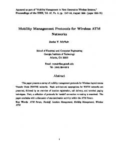
0.956Mb (bon), Ps = 0.627Mb (din), lY4 = 1.28Mb (mtv), rs = l.llMb (new), l?s = 1.33Mb (rat), r7 = 1.28Mb (SOC), rs = 0.471Mb (tal). It is clear from Figure 3 that there is a substantial variation among the eight queue solutions. This is caused by the burstiness of the sources, and the difficulty found in characterizing their bandwidth requirements statically. If equal QoS conditions are imposed on all sources, one has to dimension the links (buffer size and link utilization) according to the source which displays the worst behavior. This is certainly undesirable in the case at hand, where variations up to a loo-fold can be found on the statistics of the sources. Dynamic bandwidth allocation (ideal case) If the bandwidth requirements of each source are known in advance at each GOP time frame, [2] suggests a dynamic bandwidth allocation scheme, on which the total bandwidth is divided among the sources according to their instantaneous values at each GOP. In the present

0-7803-4187-2

case, it is possible to achieve lossless transmission without buffering, using a total bandwidth of 7.42 Mbps, or a link link utilization of 0.57, which correspond to a gain of 128 % over the static case. For higher values of link utilization, the bandwidth assigned to each source is computed according to the expression:

Pi(P, t> =

cfz

7i (t)

y.(t) P(P),

i = 1, *a., 8, 0 5

t

_< 1600s

21%

where

p(p)

=

4.30rbps

and -yi(t) = # of bits on the

n-thGOP,n=L&]. Figure 4 depict the mean queue sizes of the video sources for link utilizations in the range of 0.57 to 0.8. One finds a much more balanced &OS distribution among the eight sources, in comparison with the static case. The strategy described above can be employed for transport of recorded video, when the frame sizes are known in advance. In practice however, there is always a protocol processing time which has to be taken into account ([2]).

Dynamic bandwidth allocation with prediction In the case where the time series describing the video sources are not known in advance, or in the case of realtime video, it is necessary to forecast the bandwidth requirements of each source in advance. One needs a predictor of the bandwidth requirements yi(t), which we denote as ;vi(t). In which follows we utilize a simple RLS (recursive least squares) one-step-ahead predictor for each of the GOP time series, based on linear autoregressive models of order 12. We emphasize that our objective here is not to perform a detailed investigation of models for video traffic (eg. [l]), but rather to illustrate a practical application of forecasting technology in the context of ATM networks. It is verified in [2] that Pi-Sigma Neural Networks perform considerably better than linear RLS for the forecast of video traces. The bandwidth assigned to each source in this case is given by:

5%(t) Pi(P,t) = cfzl ‘ri(t)

P(P),

i = 1,. . . ,8,

where p(p) = 4’30rbps and Ti(t)

0 I t I 1600s

= one-step-ahead

pre-

dictor of the # of bits on the n - th GOP, n = [&I. Figure 5 depicts the mean queue sizes in the range 0.25 to 0.8. While the QoS measurements (queue sizes and corresponding delays) are obviously worse than those obtained in the ideal case, the degradation in performance is not substantial, considering the simplicity of the predictive model utilized. As an example, notice that mean queue sizes of the order of 20 cells are obtained for p = 0.75 in the ideal case, and p = 0.65 using predictions.

0000

Proc. of the 36th IEEE CDC San Diego, Ca. Dec., 1997

TP-01 3:00 5

Summary

The promise of ATM will be fulfilled only when the diverse set of traffic can be managed properly on network$of limited resources. The traffic patterns in ATM will be quite dynamic because the sources are diverse (eg, constant bit rate service, bursty compressed video, delay-insensitive internet packets). We have discussed techniques which can adapt themselves to these changing patterns in order to provide a high quality of service while maintaining high network utilization.

References

I

[l] A. Adas. Trafhc models in broadband networks. IEEE Communications Magazine, 3582-89, 1997. [2] S. Chong, S.-Q. Li, and J. Ghosh. Dynamic bandwidth allocation for efficient transport of real-time VBR video over ATM. IEEE Journal on Selected Areas in Communications, 13:12-23, 1995.





2;*b

! 0.3

Figure

0.34 0.32 0.34 owemu Link“lllliZ~“.”

*,te! 0.38

3: The mean queue size for static

1 0.42

0.4

allocation

EynPmr a1bcaoo”: Mean queue *,z*

[3] A. Elwalid, D. Mitra, and R. H. Wentworth. A new approach for allocating buffers and bandwidth to heterogeneous regulated traffic in an atm IEEE Selected Areas in Communications, node. 3(6):1115-1127, August 1995. [4] R.K. Mehra, B. Ravichandran, and R.S. Sutton. Adaptive intelligent scheduling for ATM networks. In Proceedings of the Ninth Yale Workshop on Adaptive and Learning Systems, pages 106-111, June 1996. Statistical properties of MPEG video [5] 0. Rose. traffic and their impact on traffic modeling in ATM systems. Technical Report 101, University of Wuerzburg, Institute of Computer Science, FebruVideo traces available at ftp://ftpary 1995. infoXinformatik.uni-wuerzburg.de/pub/MPEG/.

Figure

4: The mean queue size for dynamic

allocation

wnamcauocalbn With pr&lcllo” Meal7 : quweI&e

;;;;

[6] D. B. Schwartz. Learning from rare events: dynamic cell scheduling from ATM networks. In Telecommunication Application of Neural Networks. Kluwer, 1993. [7] J. Walrand and P. Varaya. High-Performance Communication Networks. Morgan Kaufmann Publishers, Inc., first edition, 1996.

Learning from Delayed [8] C.H. Watkins. PhD thesis, Cambridge University, 1989.

Rewards.

Telecommunications modeling: the [9] P.E. Wirth. brave new world. In Proceedings of the 35th IEEE Conference on Decision and Control, pages 23792380, December 1996.

0-7803-4187-2

=mois

I

I

queue size for dynamic

allocation

B WJ4020-

Figure 5: The mean with prediction

0000